An Exponential Model for Infinite Rankings

An Exponential Model for Infinite Rankings

Marina Meil˘a MMP@STAT.WASHINGTON.EDU

Le Bao LEBAO@STAT.WASHINGTON.EDU

Department of Statistics University of Washington Seattle, WA 98195-4322, USA

Editor: David Blei

Abstract

This paper presents a statistical model for expressing preferences through rankings, when the num-ber of alternatives (items to rank) is large. A human ranker will then typically rank only the most preferred items, and may not even examine the whole set of items, or know how many they are. Similarly, a user presented with the ranked output of a search engine, will only consider the highest ranked items. We model such situations by introducing a stagewise ranking model that operates with finite ordered lists called top-t orderings over an infinite space of items. We give algorithms to estimate this model from data, and demonstrate that it has sufficient statistics, being thus an expo-nential family model with continuous and discrete parameters. We describe its conjugate prior and other statistical properties. Then, we extend the estimation problem to multimodal data by intro-ducing an Exponential-Blurring-Mean-Shift nonparametric clustering algorithm. The experiments highlight the properties of our model and demonstrate that infinite models over permutations can be simple, elegant and practical.

Keywords: permutations, partial orderings, Mallows model, distance based ranking model,

expo-nential family, non-parametric clustering, branch-and-bound

1. Introduction

The stagewise ranking model of Fligner and Verducci (1986), also known as generalized Mallows

(GM), has been recognized as particularly appropriate for modeling the human process of ranking.

This model assigns a permutation πover n items a probability that decays exponentially with its distance to a central permutationσ. Here we study this class of models in the limit n→∞, with

the assumption that out of the infinitely many items ordered, one only observes those occupying the first t ranks.

the difference between the standard and the Infinite GM models. By these examples, we argue that the Infinite GM corresponds to realistic scenarios. An even more realistic scenario, that we will not tackle for now, is one where a voter (ranker) does not have access to the whole population of items (e.g., a search engine only orders a subset of the web, or a reviewer only evaluates a subset of the submissions to a conference).

After defining the infinite GM model, we show that it has sufficient statistics and give algorithms for estimating its parameters from data in the Maximum Likelihood (ML) framework. To be noted that our model will have an infinite number of parameters, of which only a finite number will be constrained by the data from any finite sample.

Then, we consider the non-parametric clustering of top-t ranking data. Non-parametric cluster-ing is motivated by the fact that in many real applications the number of clusters is not known and outliers are possible. Outliers are known to throw off estimation in an exponential model, unless the tails are very heavy. We introduce an adapted version of the well known Gaussian Blurring Mean-Shift algorithm (Carreira-Perpi˜n´an, 2006) (GBMS) that we call exponential blurring Mean Shift (EBMS).

2. The Infinite Generalized Mallows Model

In this section, we give definitions of key terms used in the article and introduce the Infinite

Gener-alized Mallows (IGM) model.

2.1 Permutations, Infinite Permutations and top-t Orderings

A permutationσ is a function from a set of items{i1,i2, . . .in} to the set of ranks 1 : n. W.l.o.g. the set of items can be considered to be the set 1 : n. Thereforeσ(i)denotes the rank of item i and σ−1_{(j)denotes the item at rank j inσ.}

There are many other ways to represent permutations, of which we will use three, the ranked

list, the matrix and the inversion table representation; all three will be defined shortly.

In this paper, we consider permutations over a countable set of items, assumed for convenience to be the the set of positive natural numbersP_{={1,2, . . . ,i. . .}. It is easy to see that the notations}

σ(i),σ−1(j)extend immediately to countable items. This will be the case with the other definitions; hence, from now on, we will always consider that the set of items isP_.

Any permutationσcan be represented by the (infinite) ranked list(σ−1(1)|σ−1(2)|. . .|σ−1(j)|

. . .). For example, letσ= (2|3|1|5|6|4|. . .|3n−1|3n|3n−2|. . .). Thenσ(1) =3 means that item 1 has rank 3 in this permutation;σ(2) =1 means that item 2 has rank 1, etc. Conversely,σ−1(1) =2 andσ−1(3 j) =3 j−2 mean that the first in the list representation ofσis item 2, and that at rank 3 j is to be found item 3 j−2, respectively. Often we will call the list representation of a permutation an ordering.

A top-t ordering πis the prefix(π−1(1)|π−1(2)|. . .|π−1(t))of some infinite ordering. For in-stance, the top-3 ordering of the aboveσis(2|3|1).

A top-t ordering can be seen as defining a set consisting of those infinite orderings which start with the prefix π. If we denote by

S

S

S

S

S

ideal infinite objects denoted byσ, and observed orderings, denoted byπ, which by virtue of being observed, are always top-t , that is, truncated. Hence, unless otherwise stated, π will denote a top-t ordering, whileσwill denote an infinite permutation.

2.2 The Permutation Matrix Representation and the Inversion Table

Now we introduce the two other ways use to represent permutations and top-t orderings.

For any σ, the permutation matrixΣcorresponding toσ hasΣi j =1 iffσ(i) = j andΣi j =0

otherwise. Ifσis an infinite permutation,Σwill be an infinite matrix with exactly one 1 in every row and column. For two permutations σ,σ′ overP_{, the matrix product} ΣΣ′ _{corresponds to the}

function compositionσ′◦σ.

The matrixΠof a top-t orderingπis a truncation of some infinite permutation matrixΣ. It has

t columns, each with a single 1 inπ−1(j), for j=1 : t.

For example, ifσ= (2|3|1|7|4|. . .)andπ= (2|3|1)is its top-3 ordering, then

Σ =



    

0 0 1 0 0 . . .

1 0 0 0 0 . . .

0 1 0 0 0 . . .

0 0 0 0 1 . . .

. . . .



    

and Π =



    

0 0 1 1 0 0 0 1 0 0 0 0

. . . .



    

. (1)

For a permutationσand a top-t orderingπ, the matrixΣTΠcorresponds to the list of ranks inσof the items inπ. In this context, one can considerσas a one-to-one relabeling of the setP_.

The inversion table of a permutationσ, with respect to the identity permutation id is an infinite sequence of non-negative integers (s1,s2, . . .) which are best defined algorithmically and recur-sively. We consider the ranked list(1|2|3|. . .). In it, we findσ−1(1)the first item ofσ, and count how many positions past the head of the list it lies. This is s1, and it always equalsσ−1(1)−1. Then we delete the entryσ−1(1)from the list, and look upσ−1(2); s2is the number of positions past the head of this list where we findσ−1(2). We then deleteσ−1(2)as well and proceed to findσ−1(3), which will give us s3, etc. By induction, it follows that an infinite permutation can be represented uniquely by the list(s1,s2, . . .). Hence sj∈ {0,1,2, . . .}, and, denoting by 1[p]the function which is

1 if the predicate p is true and is 0 otherwise, we have

sj(σ) = σ−1(j)−1−

∑

1_[σ−1_(j′_)<σ−1_(j)].

It is also easy to see that, ifπis a top-t ordering, it can be uniquely represented by an inversion table of the form(s1, . . .st). Ifπis the top-t ordering of an infinite permutationσ, then the inversion table

ofπis the t-prefix of the inversion table ofσ. This property makes the inversion table particularly convenient for our purposes.

For example, ifσ= (2|3|1|7|4|. . .)andπ= (2|3|1), then s1(σ) =s1(π) =1, s2(σ) =s2(π) =1,

s3(σ) =s3(π) =0, s4(σ) =3, s5(σ) =0, etc.

Another property of the inversion table is that it can be defined with respect to any infinite permutation σ0, by letting the ordered list corresponding to σ0 replace the list (1|2|3|. . .) in the above definition of the inversion table as follows:

sj(σ|σ0) = σ0(σ−1(j))−1−

∑

1_[σ0(σ−1_(j′_))<σ

0(σ−1(j))]. (2)

In other words, 1+sj is the rank ofσ−1(j)inσ0

P_\{σ−1_(1),...σ−1_(j−1)}.

In matrix representation, s1(σ|σ0) is the number of 0’s preceding the 1 in the first column of ΣT

0Σ; after we delete the row containing this 1, s2(σ|σ0)is the number of 0’s preceding the 1 in the second column, and so on. For a top-t orderingπ, this operation is done on the matrixΣT

0Π. For example, forπ= (3|2|1)andσ0= (3|4|2|1|. . .)the matrix representation is

ΣT

0Π =



    

1 0 0 0 0 0 0 1 0 0 0 1

. . . .



    

,

and s1(π|σ0) =0,s2(π|σ0) =1,s3(π|σ0) =1.

If σ0 is given, π is completely determined by the inversion table s1:t(π|σ). Equation (2) can be interpreted as a recursive algorithm to constructπfromσ, which we briefly describe here. We imagineσto be an ordered list of available items. From it, we choose the first rank inπby skipping the first s1ranks inσand pickingπ−1(1) =σ−1_(s

1+1). Onceπ−1(1)is picked, this item is deleted from the ordering σ. From this new list of available items, the second rank in π is picked by skipping the first s2 ranks, and chosing the item in the(s2+1)-th rank. This item is also deleted, and one proceeds to chooseπ−1(3),π−1(4), . . .π−1_{(t), etc. in a similar manner. This reconstruction} algorithm proves that the representation(s1:t)uniquely determinesπ. It is also easy to see that ifπ is a prefix ofσ, that is, ifπ−1(j) =σ−1(j)for j=1 : t, then s1=s2=. . .=st =0.

For an example we now show how to reconstructπ= (3|2|1)usingσ= (3|4|2|1|. . .). Recall that the inversion table ofπis given by s1(π|σ) =0,s2(π|σ) =1,s3(π|σ) =1.

Stage π σ Comments

Initial () (3|4|2|1|. . .)

j=1 (3) (63|4|2|1|. . .) Skip s1=0 ranks fromσ, then assign the current item toπ−1(1)

j=2 (3|2) (63|4|62|1|. . .) Skip s2=1 ranks fromσ, then assign the current item toπ−1(2)

j=3 (3|2|1) (63|4|62|61|. . .) Skip s3=1 ranks fromσ, then assign the current item toπ−1(3)

The definition of the inversion table s is identical to the first equation of Section 3 from Fligner and Verducci (1986). A reciprocal definition of the inversion table is used by Meil˘a et al. (2007) and Stanley (1997) and is typically denoted by(V1,V2, . . .). The “V” form of the inversion table is closely related to the inversion table we use here. We discuss this relationship in Section 7.

2.3 Kendall Type Divergences

For finite permutations of n itemsπandσ,

dK(π,σ) = n−1

∑

sj(π|σ) = n−1

∑

denotes the Kendall distance (Mallows, 1957) (or inversion distance) which is a metric. In the above, the index j runs only to n−1 because for a finite permutation, sn≡0. The Kendall distance

represents the number of adjacent transpositions needed to turn π into σ. An extension of the Kendall distance which has been found very useful for modeling purposes was introduced by Fligner and Verducci (1986). It is

d_θ(π,σ) =

n−1

∑

θjsj(π|σ),

withθ= (θ1, . . .θn−1)a vector of real parameters, typically non-negative. Note that dθis in general

not symmetric, nor does it always satisfy the triangle inequality. For the case of countable items, we introduce the divergence

dθ(π,σ) =

t

∑

θjsj(π|σ), (3)

where πis a top-t ordering, σis a permutation in

S

Whenθj are all equal dθ(π,σ)is proportional to the Kendall distance betweenσand the set of

orderings compatible withπand counts the number of inversions needed to makeσcompatible with π. In general, this “distance” between a top-t ordering and an infinite ordering is a set distance.2

2.4 A Probability Model over top-t Rankings of Infinite Permutations

Now we are ready to introduce the Infinite Generalized Mallows (IGM) model. We start with the observation that as any top-t ordering can be represented uniquely by a sequence of t natural num-bers, defining a distribution over the former is equivalent to defining a distribution over the latter, which is a more intuitive task. In keeping with the GM paradigm of Fligner and Verducci (1986), each sj is sampled independently from a discrete exponential with parameterθj>0.

P(sj) =

1 ψ(θj)

e−θjsj_{, s}

j =0,1,2, . . . . (4)

The normalization constantψis

ψ(θj) =

∞

∑

e−θjk₌ 1

1−e−θj, (5)

and the expectation of sj is E[sj|θj] = e −θj 1−e−θj =

1

eθj₋₁ the well known expectation of the discrete geometric distribution. Now we fix a permutation σ. Since anyπ is uniquely defined by σand the inversion table s1:t(π|σ), Equations (4) and (5) define a distribution over top-t orderings, by

P_θ,σ(π) =∏tj=1P(sj(π|σ)). This is equivalent to Pθ,σ(π) = e−∑

t

j=1[θjsj(π|σ)+lnψ(θj)]_{. (6)}

1. Definition 3 can be easily extended to a pairσ,σ′∈S_P, but in this case the divergence will often take infinite values.

2. A set distance, often called “distance” between two sets, is the minimum distance between elements in different sets,

that is,δ(A,B) =minx∈A,y∈Bδ(x,y)for a metric or divergenceδ. The set distance is not a metric, as it can easily be

The above Pθ,σ(π)has a t-dimensional real parameterθand an infinite-dimensional discrete param-eterσ. The normalization constant∏t_j=1ψ(θj)ensures that

∑

π∈top-t orderings ofP

P_θ,σ(π) = 1.

In contrast with the finite GM, the parametersθj must be strictly positive for the probability

distri-bution to exist. The most probableπfor any given t has s1(π|σ) =. . .=st(π|σ) =0. This is the

top-t prefix ofσ.

The permutationσis called the central permutation of P_θ,σ. The parametersθcontrol the spread around the modeσ. Largerθjcorrespond to more concentrated distributions. These facts are direct

extensions of statements about the GM model from Fligner and Verducci (1986) and therefore the detailed proofs are omitted.

What is different about the IGM model definition w.r.t its finite counterpart is that the parameter σis now an infinite sequence instead of a finite one. Another difference is the added condition that θj >0 which ensures thatψ(θj) is finite. This condition is not necessary in the finite case, which

leads to the non-identifiability3of the parameterσ.

If θ1=θ2 =. . .=θthe IGM model is called a single parameter IGM model. In this case

Equation (6) simplifies to

Pθ,σ(π) = e−θ∑ t

j=1sj(π|σ)−t lnψ(θ)_.

2.5 The IGM Model is a Marginal Distribution

Any top-t orderingπstands for a set of infinite sequences starting with s1:t(π|σ). Therefore, Pθ,σ(π) can be viewed as the marginal of s1:t in the infinite product space defined by the distribution

Pθ,σ(s) = e−∑

∞

j=1[θjsj+lnψ(θj)] _{s∈N×N×. . . .}

Because every infinite sequence s uniquely determines an infinite permutation, the distribution (6) also represents the probability of theπelement of the right coset

S

S

Note also that the expected value of sjis the mean of the geometric distribution E[sj] = _eθj1₋₁ ≡ ξj. Thus, the mean value parametrization of the IGM can be easily derived (proof omitted):

P_ξ,σ(π) =

t

∏

j=1

ξsj(π|σ)

j

(ξj+1)sj(π|σ)+1

. (7)

It is clear by now that the IGM P_θ,σ is an exponential family model over the sample space

(s1,s2, . . .) (note that hereσplays no role). It is also evidently an exponential family model inθ

over complete or top-t permutations. The next section will demonstrate that, less evidently, the IGM is in fact in the exponential family with respect to the discrete parameterσas well.

3. The non-identifiability of the GM model is however not a severe problem for estimation, and can be removed by

3. Estimating the Model From Data

We are given a set of N top-t orderings

S

S

sampled independently from a P_θ,σ with unknown parameters. We propose to estimateθ,σfrom this data in the ML paradigm. We will start by rewriting the log-likelihood of the model, in a way that will uncover a set of sufficient statistics. Then we will show how to estimate the model based on the sufficient statistics.

3.1 Sufficient Statistics

For any square (infinite) matrix A∈RP×P_{, denote by L(A) =}∑_{i>jAi jthe sum of the elements below}

the diagonal of A. Let L_σ(A) =L(ΣT_{AΣ), and let 1 be a vector of all 1’s. For any π, let t}

π be its length and denote tmax=maxS_N tπ, T =∑S_Ntπ, and by n the number of distinct items observed in

the data. As we shall see, tmaxis the dimension of the concentration parameter θ, n is the order of

the estimated central permutationσ, and T counts the total number of items in the data, playing a role akin to the sample size.

Proposition 1 Let{Nj,qj,Qj}j≥0represent the following statistics: Njis the number ofπ∈

S

number of times i is observed in rank j in the data

S

Qii′_,j counts how many timesπ(i) = j andπ(i′)<j. Then,

ln Pθ,σ(

S

∑

[θjLσ(Rj) +Njlnψ(θj)] with Rj = qj1T−Qj, (8)

To prove this result, we first introduce an alternative expression for the inversion table sj(π|σ).

Let the data set

S

Proposition 2

sj(π|σ) = Lσ(qj(π)1T−Qj(π)). (9)

Proof Let Q0be the infinite matrix that has 1 above the main diagonal and 0 elsewhere,(Q0)i j=1

iff j>i and letΠ: j denote the j-th column ofΠ. It is then obvious that L(A) =trace(Q0A)for any

A.

By definition, sjrepresents the number of 0’s preceding 1 in column j, minus all the 1’s in the

submatrix(ΣTΠ₎

1:σ(π−1_{(j))−1,1: j−1}. In other words, sj(π|σ) =

∑

l≥1

(Q0ΣTΠ: j)l(1−ΣTΠ:1−ΣTΠ:2−. . .ΣTΠ: j−1)l,

= (1−

∑

j′_<j

ΣT_{Π: j}

′)TQ0ΣTΠ: j,

= 1TQ0ΣTΠ: j−

∑

j′_<j

ΠT

: j′ΣQ0ΣTΠ: j,

= trace Q0ΣT_{Π: j1}T₋

∑

traceΠ: jΠT

: j′ΣQ0ΣT,

= trace Q0ΣT[Π: j1T−

∑

Π: jΠT

: j′Σ],

= L(ΣT[Π: j1T−

∑

j′_<j

Π: jΠT

: j′]Σ) = Lσ(Π: j1T−

∑

Π: jΠT

We use the fact that multiplying left by Q0 counts the zeros preceding 1 in a column in the first equality, trace AB=trace BA in the fourth and fifth equations, and the identity 1TΣ=1T in the last equation. We now note thatΠ: j=qj(π)and∑j′_<jΠ: jΠT_{: j}′=Qj(π)and the result follows. 2

Proof of Proposition 1. The log-likelihood of

S

ln P_θ,σ(

S

∑

π∈S_N

" _t

∑

πθjsj(π|σ) +lnψ(θj) #

,

= −

∑

j≥1

"

θj

∑

π∈SN

sj(π|σ) +Njlnψ(θj) #

.

Because L_σis a linear operator, the sum overπ∈

S

L_σ[(

∑

π∈S_N

qj(π))1T−

∑

π∈S_N

Qj(π))].

It is easy to verify now that the first sum represents qjand the second one represents Qj. 2

The sufficient statistics for the single parameter IGM model are described by the following corollary.

Corollary 3 Denote

q=

∑

j

qj, Q=

∑

j

Qj, R = q1T−Q. (10)

Ifθ1=θ2=. . .=θthen the log-likelihood of the data

S

ln Pθ,σ(

S

Note that qi, Qii′ represent respectively the number of times item i is observed in the data and

the number of times item i′precedes i in the data.

Proposition 1 and Corollary 3 show that the infinite model P_θ,σ has sufficient statistics. The result is obtained without any assumptions on the lengths of the observed permutations. The data π∈

S

As the parameters θ,σof the model are infinite, the sufficient statistics Rj (or R) are infinite

matrices. However, for any practically observed data set, tmax will be finite and the total number

of items observed will be finite. Thus, Nj,Rj will be 0 for any j>tmaxand R=∑j∈PRj will have

non-zero entries only for the items observed in someπ∈

S

the observed items, one can reduce Rj to a matrix of dimension n, the number of distinct observed

items. The rest of the rows and columns of Rj will be 0 and can be discarded. So in what follows

we will assume that Rj and the other sufficient statistics have dimension n.

3.2 ML Estimation: The Case of a Singleθ

We now go on to estimateθandσstarting with the case of equalθj, that is,θ1=θ2=. . .=θ. In

this case, Equation (11) shows that the estimation ofθandσdecouple. For any fixedσ, Equation (11) attains its maximum overθat

In contrast to the above explicit formula, for the finite GM, the likelihood has no analytic solution forθ(Fligner and Verducci, 1986). The estimated value ofθincreases when Lσ(R)decreases. This has an intuitive interpretation. The lower triangle ofΣTRΣcounts the “out of order” events w.r.t. the chosen modelσ. Thus, Lσ(R) can be seen as a residual, which is normalized by the “sample size” T . Equation (12) can be re-written as Lσ(R)/T =1/(eθ−1)≡ξ. In other words, the mean

value parameterξequals the average residual. This recovers a well-known fact about exponential family models. In particular, if the residual is small, that is L_σ(R)has low counts, we conclude that the distribution is concentrated, hence has a highθ.

Estimating σML amounts to minimizing L_σ(R) w.r.t σ, independently of the value of θ. The optimalσaccording to Corollary 3 is the permutation that minimizes the lower triangular part of ΣT_RΣ. To find it we exploit an idea first introduced in Meil˘a et al. (2007). This idea is to search for

σ= (i1|i2|i3|. . .)in a stepwise fashion, starting from the top item i1and continuing down.

Assuming for a moment thatσ= (i1|i2|i3|. . .)is known, the cost to be minimized Lσ(R)can be decomposed columnwise as

L_σ(R) =

∑

l6=i1

Rli1+

∑

l6=i1,i2

Rli2+

∑

l6=i1,i2,i3

Rli3+. . . ,

where the number of non-trivial terms is one less than the dimension of R. It is on this decomposition that the search algorithm is based. Reading the above algorithmically, we can compute L_σ(R), for any givenσby the following steps

1. zero out the diagonal of R

2. sum over column i1of the resulting matrix 3. remove row and column i1

4. repeat recursively from step 2 for i2,i3, . . ..

If nowσis not known, the above steps 2, 3 become the components of a search algorithm, which works by trying every i1in turn, saving the partial sums, then continuing down for a promising i1 value to try all i2’s that could follow it, etc. This type of search is represented by a search tree, whose nodes are candidate prefixes forσ.

The search tree has n! nodes, one for each possible ordering of the observed items. Finding the lowest cost path through the tree is equivalent to minimizing Lσ(R). Branch-and-bound (BB) (Pearl, 1984) algorithms are methods to explore the tree nodes in a way that guarantees that the optimum is found, even though the algorithm may not visit all the nodes in the tree. The number of nodes explored in the search forσMLdepends on the individual sufficient statistics matrix R. It was shown by Meil˘a et al. (2007) that in the worst case, the number of nodes searched can be a significant fraction of n! and as such intractable for all but small n. However, if the data distribution is concentrated around a mode, then the search becomes tractable. The more concentrated the data, the more effective the search.

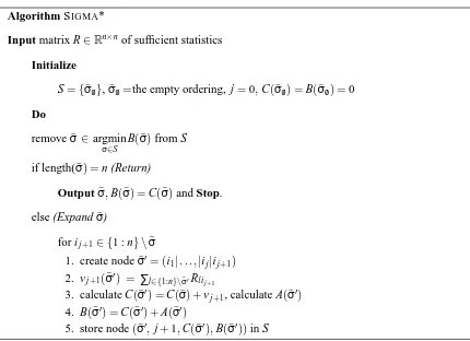
We call the BB algorithm for estimating σthe SIGMA*, by analogy with the name A∗ under which such algorithms are sometimes known. The algorithm is outlined in Figure 1. In this figure,

A is an admissible heuristic; Pearl (1984) explains their role. By default, one can use A≡0. A higher bound than 0 will accelerate the search; some of the admissible heuristics of Mandhani and Meil˘a (2009) can be used for this purpose.

standard GM model and which transfer immediately to the infinite model are the greedy search

(GREEDYR) and the the SORTR heuristic of Fligner and Verducci (1988), both described in Figure

2. The SORTR computes the costs of the first step of BB, then outputs the permutationσthat sorts these costs in increasing order. The algorithm as proposed by Fligner and Verducci (1988) also performs limited search around thisσ. For simplicity, this was not included in the pseudocode, but can be implemented easily.

The GREEDYR replaces BB with greedy search on the same sufficient statistics matrix. This

algorithm was used by Cohen et al. (1999), where a factor of 2 approximation bound w.r.t. the cost was also shown to hold.

A third heuristic is related to the special case t=1, when eachπcontains only 1 element. This is the situation of, for example, a search engine returning just the best match to a query. For t=1, as

Q is 0, the optimal ordering is the one minimizing L_σ(q1T) = [0 1. . .n−1]ΣT_{q. This is obviously}

the ordering that sorts the items in descending order of their frequency q.

In conclusion, to estimate the parameters from data in a single parameter case, one first computes the sufficient statistics, then a prefix ofσis estimated by exact or heuristic methods, and finally, with the obtained ordering of the observed items, one can compute the estimate ofθ.

3.3 ML Estimation: The Case of Generalθ

Maximizing the likelihood of the data

S

J(θ,σ) =

∑

j

[θjLσ(Rj) +Njlnψ(θj)] = Lσ(

∑

j

θjRj

| {z } Rθ

) +function ofθ. (13)

This estimation equation does not decouple w.r.tθandσ. Minimization is however possible, due to the following two observations. First, for any fixed set ofθjvalues, minimization w.r.tσis possible

by the algorithms described in the previous section. Second, for fixedσ, the optimalθjparameters

can be found analytically by

θj=ln(1+Nj/Lσ(Rj)). (14)

The two observations immediately suggest an alternating minimization approach to obtaining θML_,σML_{. The algorithm is given in Figure 3. For the optimization w.r.tσexact minimization can}

be replaced with any algorithm that decreases the r.h.s of (13). As both steps increase the likelihood, the algorithm will stop in a finite number of steps at a local optimum.4

3.4 Identifiability and Consistency Results

One remarkable property of the IGM, which is easily noted by examining the likelihood in (8) or (11), is that the data will only constrain a finite number of parameters of the model. The log-likelihood (8) depends only on the parametersθ1:tmax. Maximizing likelihood will determineθ1:tmax leaving the otherθj parameters undetermined.

4. The reader may have noted that P_θ,σis an exponential family model. For exponential family models with continuous

parameters over a convex set, the likelihood is log-concave and an iteration like the one presented here would end at

the global optimum. For our model, however, the parameterσis discrete; moreover, the set ofσ’s forms the vertices

of a convex polytope. One can show theoretically and practically that optimizing Lσ(R)can have multiple optima

Algorithm SIGMA*

Input matrix R∈Rn×n_{of sufficient statistics}

Initialize

S={σ¯_/0}, ¯σ/0=the empty ordering, j=0,C(σ¯_/0) =B(σ¯_/0) =0

Do

remove ¯σ∈argmin ¯

σ∈S

B(σ¯)from S

if length( ¯σ) =n (Return)

Output ¯σ,B(σ¯) =C(σ¯)and Stop. else (Expand ¯σ)

for ij+1∈ {1 : n} \σ¯

1. create node ¯σ′= (i1|. . . ,|ij|ij+1) 2. vj+1(σ¯′) = ∑l∈{1:n}\σ¯′R_lij+1

3. calculate C(σ¯′) =C(σ¯) +vj+1, calculate A(σ¯′)

4. B(σ¯′) =C(σ¯′) +A(σ¯′)

5. store node(σ¯′,j+1,C(σ¯′),B(σ¯′))in S

Figure 1: Algorithm SIGMA* outline. S is the set of nodes to be expanded; ¯σ= (i1|. . . ,|ij)

des-ignates a top- j ordering, that is, a node in the tree at level j. The cost of the path ¯σis given by C(σ¯) =∑j_j′₌₁∑l6∈{i1: j′}Rlil, and A(σ¯)is a lower bound on the cost to go from ¯σ, possibly 0. The total estimated cost of node ¯σis B(σ¯) =C(σ¯) +A(σ¯), which is used to predict which is the most promising path through the tree. In an implementation, node ¯σ stores: ¯σ= (i1|. . . ,|ij), j=|σ¯|,C(σ¯),B(σ¯).

Let n be the number of distinct items observed in the data. Fromσ, we can estimate at most its restriction to the items observed, that is, the restriction ofσto the setS_π∈S_N{π−1(1),π−1(2), . . . ,

π−1_(t

π)}. The next proposition shows that the ML estimate will always be a permutation which puts the observed items before any unobserved items.

Proposition 4 Let

S

S

˜

σwhich ranks all observed items before any unobserved items, so that for any parameter vector

(θ1:t), P_θ,σ(

S

S

Proof For an item i0 not observed in the data, qi0,j,Qi0i,j and Ri0i,j are 0, for any j=1 : t and any

observed item i. Hence row i0in any Rj is zero. Also note that if we switch among each other items

Algorithm SORTR

Input matrix R∈Rn×n_{of sufficient statistics with 0 diagonal}

1. compute the column sums of R, rl=∑kRkl,l=1 : n

2. sort rl,l=1 : n in increasing order

Outputσthe sorting permutation

Algorithm GREEDYR

Input matrix R∈Rn×n_{of sufficient statistics with 0 diagonal}

1. set V=1 : n the set of unused items

2. Repeat for j=1 : n−1

(a) compute rl=∑k∈VRkl,l∈V the column sums of a submatrix of R

(b) let l∗=argmin_l∈Vrl

(c) setσ−1(j) =l∗, V ←V\ {l∗}

3. setσ−1(n)to the last remaining item in V

Outputσ

Figure 2: Heuristic algorithms to estimate a central permutation: SORTR and GREEDYR. The elements Riiare never part of any sj, hence to simplify the code we assume they are set

to 0.

Algorithm ESTIMATESIGMATHETA

Input Sufficient statistics Rj,Nj, j=1 : tmax

Initial parameter valuesθ1:tmax>0

Iterate until convergence:

1. Calculate Rθ =∑jθjRj

2. Find the orderingσ=argmin_σLσ(Rθ)(exactly by SIGMA* or by heuristics)

3. Estimateθj=ln(1+Nj/Lσ(Rj))

Outputσ,θ1:tmax

The idea of the proof is to show that if we switch items i0and i the lower triangle of any Rj will

not increase, and for at least one Rj it will strictly decrease.

For this, we examine row i of some Rj. We have Qii0,j=0 and Qii0,j=qi,j. Since i is observed

then for at least one j we have Rii0,j>0. Denote byσ

′_{the permutation which is equal toσexcept}

for switching i and i0. The effect of switching i and i0on Rj is to switch elements Rii0,j and Ri0i,j.

Since the latter is always 0 and the former is greater or equal to 0, it follows that L_σ′(R_j)≤L_σ(R_j)

for any j, and that the inequality is strict for at least one j. By examining the likelihood expression in Equation (8), we can see that for any positive parametersθ1: j we have ln Pθ,σ(

S

S

By successive switches like the one described here, we can move all observed items before the unobserved items in a finite number of steps. Let the resulting permutation be ˜σ. In this process, the likelihood will be strictly increasing at each step, therefore the likelihood of ˜σwill be higher than

that ofσ. 2.

In other wordsσML is a permutation of the observed items, followed by the unobserved items in any order. Hence the ordering of the unobserved items is completely non-identifiable (naturally so). But not even the restriction ofσto the observed items is always completely determined. This can be seen by the following example. Assume the data consists of the the two top-t orderings

(a|b|c),(a|b|d). Then(a|b|c|d)and(a|b|d|c)are both ML estimates forσ; hence, it would be more accurate to say that the ML estimate ofσis the partial ordering(a|b|{c,d}). The reasonσMLis not unique over a,b,c,d in this example is that the data has no information about the relative ranking c,d, neither directly by observing c,d together in the sameπ, nor indirectly, via a third item. This

situation is likely to occur for the rarely observed items, situated near the ends of the observedπ’s. Thus this kind of inderterminacy will affect predominantly the last ranks ofσML_{. Another kind of}

indeterminacy can occur when the data is ambiguous w.r.t the ranking of two items c,d, that is,

when Rcd =Rdc>0. This situation can occur at any rank, and will occur more often for values of

theθj parameters near 0. However, observing more data mitigates this problem. Also, since more

observations typically increase the counts more for the first items inσ, this type of indeterminacy is also more likely to occur for the later ranks ofσML.

Thus, in general, there is a finite set of permutations of the observed items which have equal likelihood. We expect that these permutations will agree more on their first ranks and less in the last ranks. The exact ML estimation algorithm SIGMA* described here will return one of these permutations.

We now discuss the convergence of the parameter estimates to their true values. The IGM model has t real parameters θj,j=1 : t and a discrete and infinite dimensional parameter, the

central permutationσ. We give partial results on the consistency of the ML estimators, under the assumption that the true model is an IGM model and that t the length of the observed permutations is fixed or bounded.

Before we present the results, we need to make some changes in notation. In this section we will denote by ˆq,_Rˆ_{,etc the statistics obtained from a sample, normalized by the sample size N. We} use q,R, etc for the asymptotic, population based expectation of a statistic under the true model Pid,θ (single parameter or multiple parameters as will be the case). For instance ˆqi,j=∑π∈S_Nqi,j(π)/N

represents the frequency of i appearing in position j in the sample, while qi,j is the probability of

this event under Pid,θ. For simplicity of notation, the dependence of N is omitted.

We will show that under weak conditions, the statistics of the type q,Q,R converge to their

Proposition 5 Letσ be any infinite permutation. If the true model is Pid,θ (multiple parameters)

and t is fixed, then limN→∞Lσ(Rˆj) =Lσ(Rj)for any j=1 : t.

Since we can assume w.l.o.g. that the central permutation of the true model is the identity permu-tation, this proposition implies that for any IGM, with single or multiple parameters, and for anyσ, the statistics L_σ(_Rˆ_{j)are consistent when t is constant.}

Proposition 6 If the true model is Pid,θ (multiple or single parameter) and t is fixed, then for any

infinite permutationσ, denote by ˆθj(σ)(or ˆθ(σ))the ML estimate ofθj(orθ) given that the estimate of the central permutation isσ. Then for j=1 : t

lim

N→∞ ˆ

θj(σ) = θj(σ),

lim

N→∞ ˆ

θ(σ) = θ(σ),

where the limits should be taken in the sense of convergence in probability.

Proposition 7 Assume that the true model is Pid,θ, t is fixed, andθj ≥ θj+1 for j=1 : t−1. Let σ6=id be an infinite permutation. Then, P[Lid(Rˆj)<Lσ(Rˆj)]→1. Consequently, P[Lid(Rˆ)<

L_σ(_Rˆ_)]→1.

The consequences of these results are as follows. Assume the true model has a single parameter, and we are estimating a single parameter IGM model. Then, the likelihood of an infinite permutationσ is given by ˆR=∑t

j=1Rˆj. By Proposition 7, for anyσother than the true one, the likelihood will be

lower than the likelihood of the true permutation, except in a vanishingly small set of cases. This result is weaker than ideal, since ideally we would like to prove that the likelihood of the trueσ is higher than that of all other permutations simultaneously. We intend to pursue this topic, but to leave the derivation of stronger and results for a further publication.

Proposition 6 shows that, if the correctσis known, then theθj parameters, or alternatively the

singleθparameter, are consistent.

In the multiple parameter IGM case, for any fixed θ, the likelihood of σ is given by ˆR=

∑t

j=1θjRˆj. Hence, by Proposition 7, in this case too, for any givenσdifferent from the true central

permutation, the likelihood ofσwill be lower than the likelihood of the true model permutation. The reader will note that these results can be easily extended to the case of bounded t.

4. Non-parametric Clustering

The above estimation algorithms can be thought of as finding a consensus ordering for the ob-served data. When the data have multiple modes, the natural extension to optimizing consensus is clustering, that is, finding the groups of the population that exhibit consensus.

Algorithm EBMS

Input Top-t orderings

S

1. Forπi∈

S

2. Reduce data set by counting only the distinct permutations to obtain reduced ˜

S

counts Ni≥1 for each orderingπi∈

S

3. Forπi,πj∈

S

4. (Optional, ifθnot given in input) Setθby solving the equation

Eθ[d(

S

−θ

1−e−θ− tπ

∑

je−θ

1−e−jθ

where we set Eθ[d(

S

5. Forπi∈

S

(a) Forπj∈

S

(c) Estimateσithe “central” permutation that optimizes ¯Ri

(exactly or by heuristics) (d) Setπi ← σi(1 : tπ)

6. Go to step 2, until noπichanges.

Output ˜

S

Figure 4: The EBMS algorithm.

Nonparametric clustering is motivated by the fact that in many real applications the number of clusters is unknown and outliers exist. We consider an adapted version of the well known blur-ring mean-shift algorithm for ranked data (Fukunaga and Hostetler, 1975; Cheng, 1995; Carreira-Perpi˜n´an, 2006). We choose the exponential kernel with bandwidth 1_θ >0: K_θ(π,σ) = e−θd(π,σ)

ψ(θ) .

Under the Kendall distance dK(π,σ)the kernel has the same form as the one parameter Mallows’

model. The kernel estimator ofπiis given by

ˆr(πi) = n

∑

K_θ(πi,πj)

∑n

k=1Kθ(πi,πk)

πj= n

∑

e−θdK(πi,πj) ∑n

k=1e−θdK(πi,πk) πj,

which does not depend on the normalizing constantψ(θ)in Mallows’ model.

“attracted” towards its closest neighbors; as the shifting is iterated the data collapse into one or more clusters. The algorithm has a scale parameter θ. The scale influences the size of the local neighborhood of a top-t ordering, and thereby controls the granularity of the final clustering: for small θvalues (large neighborhoods), points will coalesce more and few large clusters will form; for largeθ’s the orderings will cluster into small clusters and singletons. In the EBMS algorithm, we estimate the scale parameterθat each iteration by solving the equation in step (d).

Practical experience shows that blurring mean-shift merges the points into compact clusters in a few iterations and then these clusters do not change but simply approach each other until they eventually merge into a single point (Carreira-Perpi˜n´an, 2006). Therefore, to obtain a meaningful clustering, a proper stopping criterion should be proposed in advance. For ranked data, this is not the case: since at each iteration step we round the local estimator into the nearest permutation, the algorithm will stop in a finite number of steps, when no ordering moves from its current position. Moreover, because ranked data is in a discrete set, we can also perform an accelerating process. As soon as two or more orderings become identical, we replace this cluster with a single ordering with a weight proportional to the cluster’s number of members. The total number of iterations remains the same as for the original exponential blurring mean-shift but each iteration uses a data set with fewer elements and is thus faster.

In the algorithm one evaluates distances between top-t orderings. There are several ways in which to turn dK(π,σ)into a d(π1,π2), where both terms are top-t orderings, containing different

sets of items. Critchlow (1985) studied them, and here we adopt for d(π1,π2)what is called the set distance, that is, the distance between the sets of infinite orderings compatible withπ1respectively π2.

We chose this formulation rather than others because this distance equals 0 whenπ1=π2, and

this is good, one could even argue necessary, for clustering. In addition, it can be calculated by a relatively simple formula, inspired by Critchlow (1985). Let

A the set intersection of orderingsπ1,π2 t1,t2 lengths ofπ1,π2

B π1\A, the items inπ1not inπ2 nA,B,C the number of items in A,B,C

C π2\A, the items inπ2not inπ1 kj the index inπ1of the j-th item not in A

lj the index inπ2of the j-th item not in A

Then

d(π1,π2) = dK((π1)|A,(π2)|A) +nBnC+nBt1−

nB

∑

kj−

nB(nB−1)

2 +nCt2−

nC

∑

lj−

nC(nC−1)

2 . (15)

π1 B1 B2 −→ π˜1 B1 B2 C1 C2 C3 C4

π2 C1 C2 C3 C4 −→ π˜2 C1 C2 C3 C4 B1 B2

Figure 5: An example of obtaining two partial orderings ˜π1,π2˜ compatible respectively withπ1,π2

The intuitive interpretation of this distance is given in Figure 5. We extend π1 andπ2 to two longer orderings ˜π1,π2, so that: (i) ˜˜ π1, ˜π2have identical sets of items, (ii) ˜π1is the closest ordering to π2 which is compatible with π1, and (iii) reciprocally, ˜π2 is the closest ordering toπ1 which is compatible with π2. We obtain ˜π1 by taking all items inπ2 but not in π1 and appending them at the end of π1 while preserving their relative order. A similar operation gives us ˜π2. Then,

d(π1,π2) =dK(π1˜ ,π2˜ ), and Equation (15) expresses this value.

5. The Conjugate Prior

The existence of sufficient statistics implies the existence of a conjugate prior (DeGroot, 1975) for the parameters of model (6). Here we introduce the general form of this prior and show that computing with the conjugate prior (or posterior), is significantly harder than computing with the likelihood (6).

We shall assume for simplicity that all top-t rankings have the same t. Consequently, our pa-rameter space consists of the real positive vectorθ1:t and the discrete infinite parameterΣ.

We define the prior parameters as a set of “fictitious sufficient statistics”, by analogy with the sufficient statistics for model (6). For this we first make a few straightforward observations about the sufficient statistics qj,Qj,j=1 : t as follows:

Q1 ≡ 0,

Qii′_,j ≥ 0 for all i,i′,j,

∑

i

qi,j = Nj for all j,

Qj1 = (j−1)qj for all j>1.

Therefore

Rj = qj1T−Qj = (

Qj

1

j−111T−I

for j>1

q11T for j=1 .

Now we letνdenote the prior strength, representing the equivalent sample size, andλ1,Λj, j=2 : t

be the prior parameters corresponding to the sufficient statistics q1,Q2:t, normalized as follows. Proposition 8 Letν>0,λ1be a vector andΛj,j=2 : t denote a set of possibly infinite matrices satisfying

λ1 ≥ 0,

Λii′_,j ≥ 0 for all i,i′,j,

Λj1 = (j−1)λj for all j>1 (by definition),

1Tλj = 1 for all j. DenoteΛ={ν,λ1,Λ2:t}and

R0_j =

(

Λj

1

j−111T−I

for j>1 λ11T _{for j=1} . Define the distribution

P_Λ(σ,θ) ∝ e−ν∑tj=1[θjL(ΣTR0jΣ)+lnψ(θj)]_{, (16)}

Proof Given observed permutationsπ1:N with sufficient statistics Rj, j=1 : t, the posterior

distri-bution of(σ,θ)is updated by

P(θ,σ|Λ,π1:N) ∝ e−∑tj=1[(νLσ(R0j)+Lσ(Rj))θj+(N+ν)lnψ(θj)]_,

= e

−(N+ν)∑t j=1[θjLσ

νR0_j+R j N+ν

!

+lnψ(θj)]

.

If the hyperparametersν,λ1,Λ2:t satisfy the conditions of the proposition, then the new hyperparam-etersΛ′={ν+N,(νλ1+q1)/(ν+N),(νΛj+Qj)/(ν+N), j=2 : t}satisfy the same conditions. 2.

The conjugate prior is defined in (16) only up to a normalization constant.5 As it will be shown below, this normalization constant is not always computable in closed form. Another aspect of con-jugacy is that one prefers the conjugate hyperparameters to represent expectations of the sufficient statistics under some Pθ,σ. The conditions in Proposition 8 are necessary, but not sufficient to ensure this fact.

To simplify the notations, we write

S∗_j = Lσ(νR0_j+Rj). (17)

This notation reflects the fact that S∗_j is the counterpart in the posterior of the sj in the distribution P_θ,σ(π). If N=0, then S∗j =νLσ(R0j). The value of S∗j depends onσ and the hyperparameters,

but does not depend on θ. The following result shows that for any fixed S∗_j, the posterior can be integrated overθj in closed form.

Proposition 9 Let P_Λ(σ,θ)be defined as in (16) and S∗_j be defined by (17). Then,

P_Λ(θj|σ) = BetaS∗j,ν+1(e −θj_),

where Beta_α,βdenotes the Beta distribution.

Proof sketch Replacingψ(θj)with its value (5) yields

P_Λ(θj|σ) ∝ e−S ∗

jθj_(1−e−θj₎ν_,

from which the desired result follows by a change of variable. 2

As a consequence, we have that

P_Λ(σ) ∝

t

∏

Beta(S∗_j(σ),1+ν). (18)

In the above, the notation Beta(x,y)is used to denote the special function Beta defined as Beta(x,y) =

Γ(x)Γ(y)

Γ(x+y).

We have shown thus that closed form integration over the continuous parametersθjis possible.

The summation over the discrete parameters poses much harder problems. We list them here.

5. The general form of a conjugate prior may include factors inσandθwhich do not depend onΛ. For simplicity of

A first unsolved question is the range of the variables S∗_j. While the sj variables in the infinite

GM model are always integers ranging from 0 to infinity, the S∗_j variables can have non-integer values ifνorΛjare non-integer. The latter is almost always the case, since under the conditions of

Proposition 8,Λj is not integer unless all its elements are 0 or 1. Second,Λj must have an infinite

number of non-null entries, which may create problems for its numerical representation. And finally, there can be dependencies between S∗_j values for different j’s. Hence, the factored expression (18)

should not be interpreted as implying the independence of the S∗_j’s.

We illustrate these points by a simple example. Assume that the conjugate prior hyperparameters are equivalent to the fictitious sample{π1= (1|2|3|. . .),π2= (2|1|3|. . .)}. Then,

ν=2, λ1 =





0.5 0.5 0



 Λ2 = 



− 0.5 0

0.5 − 0

0 0 −



, Λ3 = 



− 0 0

0 − 0 1 1 −



,

R0₁ =





− 0.5 0.5 0.5 − 0.5

0 0 −



, R0₂ =





− 0 0.5

0 − 0.5 0 0 −



, R0₃ =





− 0 0

0 − 0 0 0 −



.

For this example, there are two central rankingsσ1= (1|2|3|. . .)andσ2= (2|1|3|. . .)which have the same S_1:3∗ = (1,0,0), but noσwith S∗_j ≡0. Assume now that we are given just R0_1:3,ν=2 and

S∗₁(σ) =1 for someσ. Because S₁∗+2 is the sum of ranks ofπ−11,2(1)inσ, we can easily infer that the first two items inσmust be either(1|2)or(2|1)since any otherσwill have S∗₁6=1. But, for either of these possibilities, the computation of S∗₂(σ)from R0₂gives S∗₂(σ) =0. Hence, knowing S∗₁ informs about S∗₂(in fact determines it completely), showing that S∗₁,S∗₂are not independent.

Due to the above difficulties, computing the normalization constant of the posterior is an open problem. However, under some restrictive conditions, we are able to compute the normalization constant of the posterior in closed form.

Proposition 10 If νand Λ1:t are all integer, the S∗_j variables are independent, and the range of values of S∗_j isP_then

P(S∗_j=k) = (N+ν)Beta(k+1,N+1+ν),

and consequently

PΛ,ν(θ1:t,S1:t∗ ) = (N+ν)te−∑ t

j=1[θjS∗j+(N+ν)lnψ(θj)]_. The proof is given in Appendix A.1.

Now we examine the case of a single parameter IGM. The conjugate prior is given byν>0 and a single matrix R0corresponding to the normalized sufficient statistics matrix R,

P_ν,R0(θ,σ) ∝ e−θL(Σ

T_νR0_{Σ)+tνlnψ(θ)}

, (19)

The posterior is

P_ν,R0(θ,σ|π1:N) ∝ e−L(θΣ

T_(νR0_{+R)Σ)+t(ν+N)lnψ(θ)]} .

Denote for simplicity N′=N+ν,R′= (R+νR0_)/(N+ν_),S∗_{(σ) =L}

σ(N′R′). Then, the parameter θagain follows a Beta distribution givenσ,

After integratingθout, we obtain

PN′_,R′(σ) ∝ Beta(S∗(σ),tN′+1).

Finally, let us note that that the priors in (16) and (19) are both informative with respect toσ. By replacing the term L_σ(R0_j)(respectively L_σ(R0)) with some rj >0 (respectively r>0) one can

obtain a prior that is independent ofσ, hence uninformative. However, this prior is improper.

6. Experiments

In this section, we conduct experiments on singleθestimation, generalθestimation, real data sets, and clustering.

6.1 Estimation Experiments, Singleθ

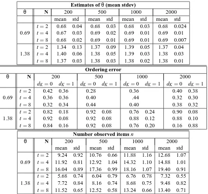
In these experiments we generated data from an infinite GM model with constant θj =ln 2,ln 4

and estimated the central permutation and the parameterθ. To illustrate the influence of t, tπ was constant over each data set. The results are summarized in Table 1.

Note that whileθappears to converge, the distance dK(σML,σ)remains approximately the same.

This is due to the fact that, as either N or t increase, n, the number of items to be ranked, increases. Thus the distance dK will be computed between ever longer permutations. The least frequent items

will have less support from the data and will be those misranked. We have confirmed this by computing the distance between the trueσand our estimate, restricted to the first t ranks. This was always 0, with the exception of n=200,θ=0.69,t=2 when it averaged 0.04 (2 cases in 50 runs) (A more detailed analysis of the ordering errors will be presented in the next subsection.)

Even so the table shows that most ordering errors are no larger than 1. We also note that the sufficient statistic R is an unbiased estimate of the expected R. Hence, for any fixed length ˜t ofσML, theσestimated from R should converge to the trueσ(see also Fligner and Verducci, 1988). The θML_{based on the true}σ_{is also unbiased and asymptotically normal.}

6.2 Estimation Experiments, Generalθ

We now generated data from an Infinite GM model withθ1=ln 2 or ln 4 andθj=2−(j−1)/2θ1for j>1. As before, tπwas fixed in each experiment at the values 2,4,8. We first look at the results for

t=8 in more detail. As the estimation algorithm has local optima, we initialized theθparameters multiple times. The initial values were (i) the constant value 0.1 (chosen to be smaller than the correct values of allθj), (ii) the constant values 1 and respectively 2 depending whetherθ1=ln 2 or

θ1=ln 4 and (iii) the trueθparameters. The case (ii) ensured that the initial point is higher than all correct values for all the estimatedθj.

Figure 6 shows the estimated values ofθj for different sample sizes N ranging in {200,500,

1000,2000}. By comparing the respective (i) and (ii) panels, one sees that the final result was insensitive to the initial values and always close to the trueθj. The results were also identical to the

results for the initialization (iii), and this was true for all the experiments we performed. Therefore, in the subsequent plots, we only display results for one initialization, (i).

Qualitatively, the results are similar to those for single θ, with the main difference stemming from the fact that, with decreasingθj values, the sampling distribution of the data is spread more,

Estimates ofθ(mean stdev)

θ N 200 500 1000 2000

mean std mean std mean std mean std

t=2 0.68 0.04 0.68 0.03 0.68 0.03 0.68 0.024 0.69 t=4 0.67 0.03 0.69 0.02 0.69 0.01 0.69 0.01

t=8 0.68 0.02 0.69 0.01 0.69 0.01 0.69 0.007

t=2 1.34 0.13 1.37 0.09 1.39 0.05 1.37 0.04

1.38 t=4 1.40 0.06 1.38 0.05 1.39 0.03 1.38 0.03

t=8 1.37 0.03 1.38 0.03 1.38 0.02 1.38 0.01

Ordering error

θ N 200 500 1000 2000

dK=0 dK=1 dK=0 dK=1 dK=0 dK =1 dK=0 dK=1

t=2 0.42 0.36 0.28 0.36 0.40 0.38

0.69 t=4 0.36 0.36 0.40 .44 0.32 0.30

t=8 0.32 0.34 0.44 0.40 0.38 0.32

t=2 0.82 0.18 0.92 0.08 0.76 0.24 0.90 0.08

1.38 t=4 0.92 0.08 0.92 0.08 0.88 0.12 0.88 0.10

t=8 0.84 0.16 0.92 0.08 0.76 0.20 0.16 0.88

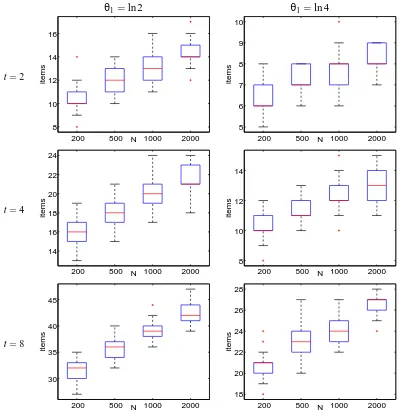
Number observed items n

θ N 200 500 1000 2000

mean std mean std mean std mean std

t=2 9.24 0.92 10.76 0.66 11.88 1.16 12.68 1.07 0.69 t=4 11.92 0.81 12.92 1.04 14.32 1.10 14.88 1.01

t=8 16.04 0.89 17.36 0.99 18.16 1.07 19.40 0.91

t=2 5.68 0.74 6.04 0.79 6.76 0.78 7.32 0.55

1.38 t=4 7.72 0.84 8.16 0.74 8.68 0.75 9.48 0.82

t=8 11.52 0.65 12.52 0.58 13.24 0.66 13.40 0.71

Table 1: Results of estimation experiments, single parameter IGM. Top: mean and standard devi-ation ofθML for two values of the true θand for different t values and sample sizes N. Middle: the proportion of cases when the ordering error, that is, the number inversions w.r.t the trueσ−1was 0, respectively 1. Bottom: number of observed items n (mean and standard deviation). Each estimation was replicated 25 or more times.

This figure allows us to observe the “asymmetry” of the error in θML. The estimates seem to biased towards larger values, especially for higher j and less data. There is a theoretical reason for this. Recall that by Equation (12)θis a decreasing function of L_σ(R). If the trueσis not optimal for the given R, due to sample variance, thenθMLwill tend to overestimateθ. HenceθMLis a biased estimate ofθ. If however, due to imperfect optimization, the estimatedσML is not optimal and has higher cost thanσ, thenθML_{will err towards underestimation. In Figures 6 and 7 the bias is always}