Boosting Algorithms for Detector Cascade Learning
Mohammad Saberian [email protected]
Nuno Vasconcelos [email protected]
Statistical Visual Computing Laboratory, University of California, San Diego La Jolla, CA 92039, USA
Editor:Yoram Singer
Abstract
The problem of learning classifier cascades is considered. A new cascade boosting algorithm, fast cascade boosting (FCBoost), is proposed. FCBoost is shown to have a number of interesting properties, namely that it 1) minimizes a Lagrangian risk that jointly accounts for classification accuracy and speed, 2) generalizes adaboost, 3) can be made cost-sensitive to support the design of high detection rate cascades, and 4) is compatible with many predictor structures suitable for sequential decision making. It is shown that a rich family of such structures can be derived recursively from cascade predictors of two stages, denoted cascade generators. Generators are then proposed for two new cascade families, last-stage andmultiplicative cascades, that generalize the two most popular cascade architectures in the literature. The concept of neutral predictors is finally introduced, enabling FCBoost to automatically determine the cascade configuration, i.e., number of stages and number of weak learners per stage, for the learned cascades. Experiments on face and pedestrian detection show that the resulting cascades outperform current state-of-the-art methods in both detection accuracy and speed.
Keywords: complexity-constrained learning, detector cascades, sequential decision-making, boosting, ensemble methods, cost-sensitive learning, real-time object detection
1. Introduction
Declared as target input
patterns Rejected
F F F
T T T
(a) (b)
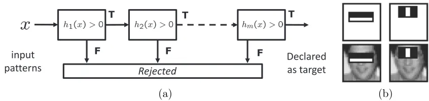
Figure 1: (a) detector cascade and (b) examples of weak learners used for face detection (Viola and Jones, 2001).
have increasing complexity, ranging from a few machine operations for h1(x) to extensive computation for hm(x). An example x is declared a target by the cascade if and only if it is declared a target by all its stages. Since the overwhelming majority of sub-windows in an image do not contain the target object, a very large portion of the image is usually rejected by the early cascade stages. This makes the average detection complexity quite low. However, because the later stages can be arbitrarily complex, the cascade can have very good classification accuracy. This was convincingly demonstrated by using the cascade architecture to design the first real-time face detector with state-of-the-art classification ac-curacy (Viola and Jones, 2001). This detector has since found remarkable practical success, and is today popular in applications of face detection involving low-complexity processors, such as digital cameras or cell phones.
Matas, 2005), and 6) joint, rather than sequential stage design (Dundar and Bi, 2007; Lefakis and Fleuret, 2010; Sochman and Matas, 2005; Bourdev and Brandt, 2005). While these advances improved the performance, the optimal design of a whole cascade is still an open problem. Most existing solutions rely on assumptions, such as the independence of cascade stages, that do not hold in practice.
In this work, we address the problem of automatically learning both the configuration and the stages of a high detection rate detector cascade, under a definition of optimality that accounts for both classification accuracy and speed. This is accomplished with thefast cascade boosting (FCBoost) algorithm, an extension of adaboost derived from a Lagrangian risk that trades-off detection performance and speed. FCBoost optimizes this risk with respect to a predictor that complies with the sequential decision making structure of the cascade architecture. These predictors are called cascade predictors, and it is shown that a rich family of such predictors can be derived recursively from a set of cascade generator
functions, which are cascade predictors of two stages. Boosting algorithms are derived for two elements of this family, last-stage and multiplicative cascades. These are shown to generalize the cascades of embedded (Xiao et al., 2003; Bourdev and Brandt, 2005; Xiao et al., 2007; Sochman and Matas, 2005; Masnadi-Shirazi and Vasconcelos, 2007; Pham et al., 2008) or independent (Viola and Jones, 2001; Schneiderman, 2004; Brubaker et al., 2008; Wu et al., 2008; Shen et al., 2011, 2010) stages commonly used in the literature. The search for the cascade configuration is naturally integrated in FCBoost by the introduction ofneutral predictors. This allows FCBoost to automatically determine 1) number of cascade stages and 2) number of weak learners per stage, by simple minimization of the Lagrangian risk. The procedure is compatible with existing cost-sensitive extensions of boosting (Viola and Jones, 2002; Masnadi-Shirazi and Vasconcelos, 2007; Pham et al., 2008; Masnadi-Shirazi and Vasconcelos, 2010) that guarantee cascades of high detection rate, and generalizes adaboost in a number of interesting ways. A detailed experimental evaluation on face and pedestrian detection shows that the resulting cascades outperform current state-of-the-art methods in both detection accuracy and speed.
2. Prior Work
A large literature on detector cascade learning has emerged over the past decade. In this section, we briefly review the main problems in this area and their current solutions.
2.1 The Problems of Cascade Learning
As illustrated in Figure 1, a cascaded detector is a sequence of detector stages. The aim is to detect instances from a target class. Examples from this class are denoted positives
while all others are denoted negatives. An example rejected, i.e., declared a negative, by any stage is rejected by the cascade. Examples classified as positives are propagated to subsequent stages. To be computationally efficient, the cascade must use simple classifiers in the early stages and complex ones later on. Under the procedure proposed by Viola and Jones (2001), the cascade designer must first select a number of stages and the target detection/false-positive rate for each stage. A high detection rate is critical, since improperly rejected positives cannot be recovered. The false-positive rate is less critical, since the cascade false-positive rate can be decreased by addition of stages, although at the price of extra computation. The stages are designed with adaboost. The target detection rate is met by manipulating the stage threshold, and the target false-positive rate by increasing the number of weak learners. This frequently leads to an exceedingly complex learning procedure. One difficulty is that the optimal cascade configuration (number of stages and stage target rates) is unknown. We refer to this as the cascade configuration problem. While some configurations have evolved by default, e.g., 20 stages, with a detection rate of 99.5% and a false-positive rate of 50%, there is nothing special about these values. This problem is compounded by the fact that, for late stages where negative examples are close to the classification boundary, it may be impossible to meet the target rates. In this case, the designer must backtrack (redesign some of the previous stages). Frequently, various iterations of parameter tuning are needed to reach a satisfactory cascade. Since each iteration requires boosting over a large set of examples and features, the process can be tedious and time consuming. We refer to this as thedesign complexity problem.
of stage false-positive rates can be used to shuffle computation between stages, there is no way to predict the amount of computation corresponding to a particular rate. This is the
complexity optimization problem.
2.2 Previous Solutions
Over the last ten years, significant research has been devoted to all of the above problems. Feature design: Viola and Jones introduced a very efficient set of Haar wavelets (Viola and Jones, 2001). They showed that these features could be extracted, with a few operations, from an integral image (cumulative image sum). While all features in the original Haar set were axis-aligned, it is possible to extent it for 45◦ rectangles, (Lienhart and Maydt, 2002). Similarly, several authors pursued extensions to other orientations (Carneiro et al., 2008; Du et al., 2006; Messom and Barczak, 2006). More recently, this has been extended to compute integral images over arbitrary polygonal regions (Pham et al., 2010). Beyond these features, integral images can also be used to efficiently compute histograms (Porikli, 2005). This reduces to quantizing the image into a set ofchannels (associated with the histogram bins) and computing an integral image per channel. For example, a computationally efficient version of the HOG descriptor (Dalal and Triggs, 2005) was then developed and used to design a real-time pedestrian detector cascade (Zhu et al., 2006). More recently, this idea has been extended to multiple other channels (Doll´ar et al., 2009). Finally, extensions have been developed for more general statistical descriptors, e.g., the covariance features (Tuzel et al., 2008). While the algorithms proposed in this work support any of these features, we adopt the Haar set (Viola and Jones, 2001). This is mostly for consistency with the cascade learning literature, where Haar wavelets are predominant.
learners, e.g., linear SVMs (Zhu et al., 2006) or decision trees of depth two (Doll´ar et al., 2009), and boosting algorithms such as realboost or logitboost (Sochman and Matas, 2005; Schneiderman, 2004; Li and Zhang, 2004; Tuzel et al., 2008).
Beyond classification performance, some attention has been devoted to design complex-ity. Since the bulk of the learning time is spent on weak learner selection, low-complexity methods have been proposed for this. For example, it is possible to trade off memory for computational efficiency (Wu et al., 2008) or to model Haar wavelet responses as Gaus-sian variables, whose statistics can be computed efficiently (Pham and Cham, 2007). While speeding up the design of each stage, these methods do not eliminate all aspects of threshold tuning, stage backtracking, etc. It could be argued that this is the worst component of design complexity, since these operations require manual supervision. A number of enhancements have been proposed in this area. While Viola and Jones proposed stage-specific threshold adjustments (Viola and Jones, 2001), it is possible to formulate threshold adjustments as an a-posteriori optimization of the whole cascade (Luo, 2005; Sun et al., 2004). These methods are hampered by the limited effectiveness of threshold adjustments when stage detectors have poor ROC performance (Masnadi-Shirazi and Vasconcelos, 2010). Better performance is usually achieved with cost-sensitive extensions of boosting, which optimize a cost-sensitive risk directly (Viola and Jones, 2002; Masnadi-Shirazi and Vasconcelos, 2007; Pham et al., 2008). More recently, Masnadi-Shirazi et al. proposed Bayes consistent cost-sensitive ex-tensions of adaboost, logitboost, and realboost (Masnadi-Shirazi and Vasconcelos, 2010). These algorithms were shown to substantially improve the false-positive performance of cascades of high detection rate (Masnadi-Shirazi and Vasconcelos, 2007). These could be combined with the methods which devise a predictor of the optimal false positive and de-tection rate for each stage, from statistics of the previous stages, so as to design a cascade of cost-sensitive stages automatically (Brubaker et al., 2008; Dundar and Bi, 2007).
Cascade configuration: Most of the above enhancements assume a known cascade configuration and sequential stage learning. This is a suboptimal design strategy and the assumed cascade configuration may not be attainable in practice. An alternative is to adopt cascades ofembedded stages where each stage is the starting point for the design of the next (Xiao et al., 2003; Bourdev and Brandt, 2005; Xiao et al., 2007; Sochman and Matas, 2005; Masnadi-Shirazi and Vasconcelos, 2007; Pham et al., 2008). The main advantage of this structure is that the whole cascade can be designed with a single boosting run, and adding exit points to a standard classifier ensemble. This also minimizes the convergence rate problems of individual stage design. Using Wald’s theory of sequential decision making, it is possible to derive a method for learning embedded stages (Sochman and Matas, 2005). While attempting to optimize the whole cascade, these approaches do not fully address the configuration problem. Some simply add an exit point per weak learner (Masnadi-Shirazi and Vasconcelos, 2007; Xiao et al., 2007; Sochman and Matas, 2005), while others use post-processing (Bourdev and Brandt, 2005; Xiao et al., 2003) or pre-specified detection and false-positive rates (Pham et al., 2008) to determine exit point locations. More recently, it is proposed to learn all stages simultaneously, by modeling a cascade as the product, or logical “AND”, of its stages (Lefakis and Fleuret, 2010; Raykar et al., 2010).
cas-cade learning can require extensive trial and error. This can be quite expensive from a computational point of view and leads to a tedious design procedure, which can produce sub-optimal cascades. In the following sections we propose an alternative framework, which is fully automated and jointly determines 1) the number of cascade stages, 2) the number of weak learners per stage, and 3) the predictor of each stage, by minimizing a Lagrangian risk that is cost-sensitive and explicitly accounts for detection speed.
3. An Extension of Adaboost for the Design of Classifier Cascades
We start with a brief review of boosting.
3.1 Boosting
A binary classifier h:X → {−1,1} maps an example x into a class labely(x). A learning algorithm seeks the classifier of minimum probability of error, PX(h(x) 6= y(x)), in the space of binary mappings
H={h|h:X → {−1,1}}.
Since H is not convex and h ∈ H not necessarily differentiable, this is usually done by restricting the search to mappings of the form
h(x) =sign[f(x)],
where f : X → R, is a predictor. The goal is then to learn the optimal f(x) in a set of predictors
F={f|f :X →R}.
This is the predictor which minimizes the classification risk,RE :F→R, RE[f] =EX,Y{L(y(x), f(x))} '
1
|St|
X
i
L(yi, f(xi)), (1)
where L:{+1,−1} ×R→ Ris a loss function, and St={(x1, y1), . . . ,(xn, yn)} is a set of training examplesxi of labels yi.
Boosting algorithms are iterative procedures that learn f as a combination of simple predictors, known as weak learners, from a set G={g1(x), . . . , gn(x)} ⊂ F. The optimal combination is the solution of
minf(x) RE[f]
s.t: f(x)∈span(G). (2)
and better generalization. Boosting can be interpreted as a greedy forward feature selection procedure to find such sparse solutions.
Although the ideas proposed in this work can be combined with most boosting al-gorithms, we limit the discussion to adaboost (Freund and Schapire, 1997). This is an algorithm that learns a predictor f by minimizing the risk of (1) when L is the negative exponential of the margin y(x)f(x)
L(y(x), f(x)) =e−y(x)f(x). (3)
This is known as the exponential loss function (Schapire and Singer, 1999).
The boosting algorithms proposed in this paper are inspired by the statistical view of adaboost (Mason et al., 2000; Friedman, 1999). Under this view, each iteration of boosting computes the functional derivatives of the risk along the directions of the weak learners
gk(x), at the current solution f(x). This can be written as
< δRE[f], g > =
d
dRE[f+g]
=0 = 1
|St|
X
i
d
de
−yi(f(xi)+g(xi))
=0 = − 1
|St|
X
i
yiwig(xi), (4)
whereyi =y(xi) and
wi =w(xi) =e−yif(xi), (5)
is the weight of example xi. The latter measures how well xi is classified by the current predictorf(x). The predictor is then updated by selecting the direction (weak learner) of steepest descent
g∗(x) = arg max
g∈G <−δRE[f], g >
= arg max g∈G
1
|St|
X
i
yiwig(xi), (6)
and computing the optimal step size along this direction
α∗ = arg min
α∈RRE[f +αg
∗]. (7)
While the optimal step size has a closed form for adaboost (Freund and Schapire, 1997), it can also be found by a line search. The predictor is finally updated according to
f(x) =f(x) +α∗g∗(x), (8)
Algorithm 1 adaboost
Input: Training setSt={(x1, y1), . . . ,(xn, yn)}, where yi∈ {1,−1} is the class label of examplexi, and number of iterations N.
Initialization: Setf(x) = 0. for t= 1 to N do
Compute <−δRE[f], g >for all weak learners using (4). Select the best weak learnerg∗(x) using (6).
Find the optimal step sizeα∗ along g∗(x) using (7). Updatef(x) =f(x) +α∗g∗(x).
end for
Output: decision rule: sign[f(x)]
3.2 Cascade Boosting
In this work, we consider the question of whether boosting can be extended to learn a detector cascade. We start by introducing some notation. As shown in Figure 1-a), a classifier cascade is a binary classifierH(x)∈Himplemented as a sequence of classifiers
hi(x) =sgn[fi(x)] i= 1, . . . , m, (9)
where the predictors fi(x) can be any real functions, e.g., linear combinations of weak learners. The cascade implements the mapping H:X → {−1,1} where
H(x) =Hm[h
1, . . . , hm](x) =
−1 if ∃k:hk(x)<0
+1 otherwise, (10)
andHm[h
1, . . . , hm] is aclassifier cascading (CC) operator,i.e., a functional mappingHm: Hm→Hof the stage classifiers h1, . . . , hm into the cascaded classifierH.1
Similarly, it is possible to define a cascade predictor F(x) for H(x), i.e., a mapping
F :X →Rsuch that
H(x) =sign[F(x)], (11)
where
F(x) =Fm[f
1, . . . , fm](x), (12)
and Fm :Fm→Fis apredictor cascading (PC) operator, i.e., a functional mapping of the stage predictorsf1, . . . , fm into the cascade predictorF. We will study the structure of this operator in Section 4. For now, we consider the problem of learning a cascade, given that the operatorFm is known.
To generalize adaboost to this problem it suffices to use the predictor F(x) in the exponential loss of (3) and solve the optimization problem
minm,f1,...fm RE[F] =
1 |St|
P
ie
−yiF(xi)
s.t: F(x) =Fm[f
1, . . . , fm](x)
∀i fi(x)∈span(G)
(13)
1. The notationHm
[h1, . . . , hm](x) should be read as: the value at xof the image of (h1, . . . , hm) under
operatorHm
by gradient descent inspan(G). The main difference with respect to adaboost is that, since any of the cascade stages can be updated, multiple gradient steps are possible per iteration. The directional gradient for updating the predictor of thekth stage is
< δRE[F], g >k=
d dRE[F
m[f
1, . . . fk+g, . . . fm]]
=0 = 1
|St|
X
i
d
de
−yiFm[f1,...fk+g,...fm](xi)
=0 = 1
|St|
X
i
(−yi)e−yiF
m[f
1,...fm](xi)
d
dF
m[f
1, . . . fk+g, . . . fm]
=0 (xi)
= − 1 |St|
X
i
yiw(xi)bk(xi)g(xi), (14)
with
w(xi) = e−yiF
m[f
1,...fm](xi)=e−yiF(xi) (15) bk(xi) =
d
dF
m[f
1, . . . fk+g, . . . fm]
=0
(xi). (16)
The optimal descent direction for the kth stage is then
g∗k = arg max
g∈G <−δRE[F], g >k
= arg max g∈G
1
|St|
X
i
yiw(xi)bk(xi)g(xi), (17)
the optimal step size along this direction is
αk∗ = arg min α∈RRE[F
m[f
1, .., fk+αgk∗, ..fm]], (18)
and the optimal stage update is
fk(x) =fk(x) +α∗g∗(x). (19)
4. The Structure of Cascade Predictors
In this section, we derive a general form for Fm. We show that any cascade is compatible with an infinite set of predictors and that these can be computed recursively. This turns out to be important for the efficient implementation of the learning algorithm of the previous section. We next consider a class of PC operators synthesized by recursive application of a two-stage PC operator, denoted the generator of the cascade. Two generators are then proposed, from which we derive two new cascade predictor families that generalize the two most common cascade structures in the literature.
4.1 Cascade Predictors
From (10), a classifier cascade implements the logical-AND of the outputs of its stage classifiers, i.e., Hm is the pointwise logical-AND ofh
1, . . . , hm,
Hm[h1, . . . , hm](x) =h1(x)∧. . .∧hm(x), (20) where∧ is the logical-AND operation. Since, from (10)-(12),
Hm[h1, . . . , hm](x) =sgn[Fm[f1, . . . , fm](x)], (21) it follows from (9) that
sign[Fm[f1, . . . , fm](x)] =sgn[f1(x)]∧. . .∧sgn[fm(x)]. (22) This holds if and only if
Fm[f
1, . . . , fm](x)<0 if ∃k:fk(x)<0
Fm[f
1, . . . , fm](x)>0 otherwise. (23)
Since (22) holds for any operator with this property, any such Fm is denoted a pointwise
soft-AND of its arguments. In summary, while a cascade implements the logical-AND of its stage decisions, the cascade predictor implements a soft-AND of the corresponding stage predictions. Note that there is an infinite number of soft-AND operators which will implement the same logical-AND operator, once thresholded according to (21). This makes the set of cascade predictors much richer than that of cascades.
4.2 Recursive Implementation
For anym, it follows from (20) and the associative property of the logical-AND that
Hm[h1, . . . , hm] =
H2[h
1, h2], m= 2
H2
h1,Hm−1[h2, . . . , hm]
m >2. (24)
A similar decomposition holds for the soft-AND operator of (23), since
sgn[Fm[f1, . . . , fm](x)] =
sgn
F2[f
1, f2](x)
, m= 2
sgn
F2
f1,Fm−1[f2, . . . , fm]
(x)
m >2. (25)
The main difference between the two recursions is that, while there is only one logical-AND
H2[f
possible to use a different operatorF2 at each level of the recursion, i.e., replaceF2 byF2 m, to synthesize all possible sequences of soft-AND operators {Fi}m
i=2 for which the left-hand side of (25) is the same. For simplicity, we only consider soft-AND operators of the form of (25) in this work.
The recursions above make it possible to derive a recursive decomposition of both the cascade and the sign of its predictor. In particular, defining
Hk(x) = Hm−k+1[hk, . . . , hm](x), (24) leads to the cascade recursion
Hk(x) =
hm(x), k=m
H2[h
k, Hk+1] (x), 1≤k < m,
withH1(x) =H(x). Similarly, for any sequence of soft-AND operators{Fi}mi=2 compatible with (25), defining
Fk(x) = Fm−k+1[fk, . . . , fm](x), leads to thepredictor recursion
sgn[Fk(x)] =
sgn[fm(x)], k=m
sgn
F2[f
k, Fk+1] (x)
, 1≤k < m, (26)
with sgn[F1(x)] =sgn[F(x)]. Simplifying (26), in the remainder of this work we consider predictors of the form
Fk(x) =
fm(x), k=m
F2[f
k, Fk+1] (x), 1≤k < m.
(27)
Since the core of this recursion is the two-stage predictor
G[f1, f2] =F2[f1, f2], (28)
this is denoted thegeneratorof the cascade. We will show that the two most popular cascade architectures can be derived from two such generators. For each, we will then derive the cascade predictors Fk(x),the cascade boosting weights w(xi) of (15), and the coefficients
bk(xi) of (16). We start by defining some notation to be used in these derivations.
4.3 Some Definitions
Some of the computations of the following sections involve derivatives of Heaviside step functionsu(.), which are not differentiable. As is common in the neural network literature, this problem is addressed with the sigmoidal approximation
u(x)≈σ(x) = 1
2(tanh(µx) + 1). (29) The parameterµcontrols the sharpness of the sigmoid. This approximation is well known to have the symmetry σ(−x) = 1−σ(x) and derivative σ0(x) = 2µσ(x)σ(−x). We also introduce the sequence ofcascaded Heaviside functions
γk(x) =
1, k= 1
Q
j<ku[fj(x)], k >1,
and cascaded rectification functions
ξk(x) =
1, k= 1
Q
j<kfj(x)u[fj(x)], k >1, (31)
where u(.) is the Heaviside step. The former generalize the Heaviside step, in the sense that γk(x) = 1 if fj(x) > 0 for all j < k and γk(x) = 0 otherwise. The latter generalize the half-wave rectifier, in the sense that γk(x) =Qj<kfj(x) if fj(x)>0 for all j < k and
γk(x) = 0 otherwise.
4.4 Last Stage Cascades
The first family of cascade predictors that we consider is derived from the generator
G1[f1, f2](x) = f1(x)u[−f1(x)] +u[f1(x)]f2(x) =
f1(x) if f1(x)<0
f2(x) if f1(x)≥0, (32)
Using (27), the associated predictor recursion is
Fk(x) =
fm(x), k=m
fk(x)u[−fk(x)] +u[fk(x)]Fk+1(x), 1≤k < m. (33)
The kth stage of the associated cascade passes example x to stage k+ 1 if f
k(x) ≥ 0. Otherwise, the example is rejected with prediction fk(x). Hence,
Fm[f1, . . . , fm](x) =
fj(x) if fj(x)<0 and
fi(x)≥0 i= 1, . . . , j−1
fm(x) if fi(x)≥0 i= 1. . . , m−1,
i.e., the cascade prediction is that of the last stage visited by the example. For this reason, the cascade is denoted alast-stage cascade.
This property makes it trivial to compute the weights w(x) of the cascade boosting algorithm, using (15). It suffices to evaluate
w(xi) =e−yifj∗(xi), (34)
respect tofk. This can be obtained by recursive application of (33), since
Fm[f1, . . . , fm](x) =F1(x)
= f1(x)u[−f1(x)] +u[f1(x)]F2(x)
= f1(x)u[−f1(x)] +u[f1(x)]{f2(x)u[−f2(x)] +u[f2(x)]F3(x)} =
k−1
X
i=1
fi(x)u[−fi(x)]
Y
j<i
u[fj(x)]
+Fk(x)
Y
j<k
u[fj(x)]
=
"k−1 X
i=1
fi(x)u[−fi(x)]γi(x)
#
+Fk(x)γk(x) k= 1. . . m
=
"k−1 X
i=1
fi(x)u[−fi(x)]γi(x)
#
+γk(x){fk(x)u[−fk(x)] +u[fk(x)]Fk+1(x)} k < m
=
"k−1 X
i=1
fi(x)u[−fi(x)]γi(x)
#
+γk(x){fk(x) +u[fk(x)][Fk+1(x)−fk(x)]}
≈ "k−1
X
i=1
fi(x)u[−fi(x)]γi(x)
#
+γk(x)fk(x) +γk(x)σ[fk(x)][Fk+1(x)−fk(x)] (35)
where γk(x) are the cascaded Heaviside functions of (30) and we used the differentiable approximation of (29) in (35). Note that neither the first term on the right-hand side of (35) nor γk orFk+1 depend on fk. It follows from (16) that
bk(x) =
γk(x), k=m
γk(x){1 + 2µσ[fk(x)][Fk+1(x)−fk(x)]}σ[−fk(x)] 1≤k < m, (36) whereσ(.) is defined in (29). Givenx, all these quantities can be computed with a sequence of a forward, a backward, and a forward pass through the cascade. The initial forward pass computesγk(x) for allkaccording to (30). The backward pass then computesFk+1(x) using (33). The final forward pass computes the weight w(x) and coefficients bk(x) using (34) and (36). These steps are summarized in Algorithm 2. The procedure resembles the back-propagation algorithm for neural network training (Rumelhart et al., 1968).
4.5 Multiplicative Cascades
The second family of cascade predictors has generator
G2[f1, f2](x) = f1(x)u[−f1(x)] +u[f1(x)]f1(x)f2(x) =
f1(x) if f1(x)<0
f1(x)f2(x) if f1(x)≥0.
(37)
Using (27), the associated predictor recursion is
Fk(x) =
fm(x), k=m
fk(x)u[−fk(x)] +u[fk(x)]fk(x)Fk+1(x), 1≤k < m
Algorithm 2 Last-stage cascade
Input: Training example (x, y), stage predictors fk(x), k= 1, . . . , m, sigmoid parameter
µ.
Evaluation: Set γ1(x) = 1. for k= 2 to m do
Setγk(x) =γk−1(x)u[fk(x)]. end for
Set Fm(x) =fm(x). for k=m−1 to 1do
SetFk(x) =fk(x)u[−fk(x)] +u[fk(x)]Fk+1(x). end for
Learning:
Set w(x) =e−yfj∗(x) wherej∗ is the smallestk for whichf
k(xi)<0 and j∗ =m if there is no suchk.
for k= 1 to m−1do
Setbk(x) =γk(x){1 + 2µσ[fk(x)][Fk+1(x)−fk(x)]}σ[−fk(x)]. end for
Set bk(x) =γm(x).
Output: w(x),{Fk(x), bk(x)}mk=1.
and
Fm[f1, . . . , fm](x) =
Q
i≤jfi(x) if fj(x)<0 and
fi(x)≥0 i= 1..j−1
Qm
i=1fi(x) if fi(x)≥0 i= 1..m−1.
Hence, the cascade predictor is the product of all stage predictions up-to and including that where the example is rejected. This is denoted amultiplicative cascade.
The weights w(x) of the cascade boosting algorithm are
w(xi) =e−yi
Q
k≤j∗fk(xi),
respect tofk. This can be obtained by recursive application of (38), since
Fm[f1, . . . , fm](x) =F1(x)
= f1(x)u[−f1(x)] +u[f1(x)]f1(x)F2(x)
= f1(x)u[−f1(x)] +u[f1(x)]f1(x){f2(x)u[−f2(x)] +u[f2(x)]f2(x)F3(x)} =
k−1
X
i=1
fi(x)u[−fi(x)]
Y
j<i
fj(x)u[fj(x)]
+Fk(x)
Y
j<k
fj(x)u[fj(x)]
=
"k−1 X
i=1
fi(x)u[−fi(x)]ξi(x)
#
+Fk(x)ξk(x) k= 1. . . m
=
"k−1 X
i=1
fi(x)u[−fi(x)]ξi(x)
#
+ξk(x){fk(x)u[−fk(x)] +u[fk(x)]fk(x)Fk+1(x)} k < m
=
"k−1 X
i=1
fi(x)u[−fi(x)]ξi(x)
#
+ξk(x)fk(x){1 +u[fk(x)][Fk+1(x)−1]}
≈ "k−1
X
i=1
fi(x)u[−fi(x)]ξi(x)
#
+ξk(x)fk(x){1 +σ[fk(x)][Fk+1(x)−1]}, (39)
where ξi(x) are the rectification functions of (31) and we used (38) and the differentiable approximation of (29) in (39). Since neither the first term on the right hand side, ξk, or
Fk+1 depend onfk, it follows from (16) that
bk(x) =
ξm(x), k=m
ξk(x){1 +σ[fk(x)][Fk+1(x)−1]}{1 + 2µfk(x)σ[−fk(x)]} 1≤k < m,(40) where σ(.) is defined in (29). Again, these coefficients can be computed with a forward, a backward, and a forward pass through the cascade, which resembles back-propagation, as summarized in Algorithm 3.
5. Learning the Cascade Configuration
Given a cascade configuration, Algorithms 2 or 3, could be combined with the algorithm of Section 3.2 to extend adaboost to the design of last-stage or multiplicative cascades, respectively. However, the cascade configuration is usually not known and must be learned. This consists of determining the number of cascade stages and the number of weak learners per stage.
5.1 Complexity Loss
We start by assuming that the number of cascade stages is known and concentrate on the composition of these stages. So far, we have proposed to simply update, at each boosting iteration, the stagekwith the weak learnerg∗
Algorithm 3 multiplicative cascade
Input: Training example (x, y), stage predictors fk(x), k= 1, . . . , m, sigmoid parameter
µ.
Evaluation: Set ξ1= 1.
for k= 2 to m do
Setξk(x) =ξk−1(x)fk(x)u[fk(x)]. end for
Set Fm(x) =fm(x). for k=m−1 to 1do
SetFk(x) =fk(x)u[−fk(x)] +u[fk(x)]fk(x) Fk+1(x). end for
Learning:
Set w(x) =e−yQk≤j∗fk(x) wherej∗ is the smallestk for whichf
k(xi)<0 and j∗ =m if there is no such k.
for k= 1 to m−1do
Setbk(x) =ξk(x){1 +σ[fk(x)][Fk+1(x)−1]}{1 + 2µfk(x)σ[−fk(x)]}. end for
Set bm(x) =ξm(x).
Output: w(x),{Fk(x), bk(x)}mk=1.
and classification speed. To guarantee such a trade-off it is necessary to search for the most accurate detector under a complexity constraint. This can be done by minimizing the Lagrangian
L[F] = RE[F] +ηRC[F], (41)
whereF(x) andRE[F] are the cascade predictor and classification risk of (13), respectively,
RC[F] = EX|Y{LC(F, x)|y(x) =−1} ' 1
|St−| X
xi∈St−
LC(F, xi),
is a complexity risk and η a Lagrange multiplier that determines the trade-off between accuracy and computational complexity. RC[F] is the empirical average of a computa-tional loss LC(F, x),which reflects the number of machine operations required to evaluate
F(x) =Fm[f
1, . . . , fm](x), over the set St− of negatives in St. The restriction to negative examples is not necessary but common in the classifier cascade literature, where computa-tional complexity is usually defined as the average computation required to reject negative examples. This is mostly because positives are rare and contribute little to the overall computation.
to the remaining stages,
C(Fk, x) =
Ω(fk) +u[fk(x)]C(Fk+1, x), k < m Ω(fm), k=m,
(42)
whereFk(x) is as defined in (27) and Ω(fk) is the computational cost of evaluating stagek. DefiningC(Fm+1, x) = 0, it follows that
C(F, x) = Ω(f1) +u[f1(x)]C(F2, x)
= Ω(f1) +u[f1(x)][Ω(f2) +u[f2(x)]C(F3, x)] =
k−1
X
i=1 Ω(fi)
Y
j<i
u[fj(x)]
+C(Fk, x) Y
j<k
u[fj(x)]
=
"k−1 X
i=1
Ω(fi)γi(x)
#
+ Ω(fk)γk(x) +u[fk(x)]C(Fk+1, x)γk(x)
= δk(x) + Ω(fk)γk(x) +θk(x)u[fk(x)], (43)
whereγi(x) are the cascaded Heaviside functions of (30) and
δk(x) = k−1
X
i=1
Ω(fi)γi(x),
θk(x) = C(Fk+1, x)γk(x). (44)
This relates the cascade complexity to the complexity of thekthstage, Ω(f
k). The surrogate computational lossLC[F, x] is inspired by the surrogate classification loss of adaboost, which upper bounds the zero-one loss u[−yf(x)] by the exponential e−yf(x). Using the bound
u[f(x)]≤ef(x) on (43) leads to
LC[F, x] = δk(x) + Ω(fk)γk(x) +θk(x)efk(x), and the computational risk
RC[F] = 1
|St−| X
xi∈St−
δk(xi) + Ω(fk)γk(xi) +θk(xi)efk(xi). (45)
To evaluate this risk, it remains to determine the computational cost Ω(fk) of the predictor of thekthcascade stage. Sincef
k(x) =Plαlgl(x), gl ∈G,is a linear combination of weak learners, we define
Ω(fk) =
X
l
Ω(gl). (46)
there is no cost in the repeated evaluation of a weak learner. For this, W(fk) is split into two sets. The first, O(fk), contains the weak learners used in some earlier cascade stage
fj, j≤k. Since the outputs of these learners can be kept in memory, they require minimal computation (multiplication byαl and addition to cumulative sum). The second is the set
N(fk) of weak learners unused in prior stages. The computational cost of fk is then
Ω(fk) =|N(fk)|+λ|O(fk)|, (47)
whereλ <1 is the ratio of computation required to evaluate a used vs. new weak learner. This implies that when updating the kth stage predictor
Ω(fk+g) = Ω(fk) +ρ(g, fk),
with
ρ(g, fk) =
λ ifg∈ O(fk) 1 ifg∈ N(fk).
(48)
5.2 Boosting with Complexity Constraints
Given the computational risk of (45), it is possible to derive a boosting algorithm that accounts for cascade complexity. We start by deriving the steepest descent direction of the Lagrangian of (41), with respect to stage k
<−δL[F], g >k = <−δ(RE[F] +ηRC[F]), g >k
= <−δRE[F], g >k+η <−δRC[F], g >k.
The first term is given by (14), the second requires the descent direction with respect to the complexity risk RC[F]. Using (45),
< δRC[F], g >k=
d dRC(F
m[f
1, .., fk+g, ..fm])
=0 = 1
|St−| X
i
ys i
d dLC[F
m[f
1, .., fk+g, ..fm], xi]
=0 = 1
|St−| X i ys i d d h
δk(xi) + [Ω(fk) +ρ(fk, g)]γk(xi) +θk(xi)efk(xi)+g(xi)
i
=0 = 1
|St−| X
i
yisψk(xi)θk(xi)g(xi), (49)
whereys
i =I(yi =−1),I(x) is the indicator function,θk(xi) as in (44) and
ψk(xi) = efk(xi). (50)
Finally, combining (14) and (49),
<−δL[F], g >k =
X
i
yiw(xi)bk(xi)
|St|
−ηy
s
iψk(xi)θk(xi)
|St−|
Algorithm 4 BestStageUpdate
Input: Training set St, trade-off parameter η, cascade [f1, . . . , fm], index kof the stage to update, sigmoid parameter µ.
for each pair (xi, yi) in St do
Computew(xi),bk(xi),Fk(xi) e.g., using Algorithm 2 for last-stage or Algorithm 3 for multiplicative cascades.
Compute θk(xi),ψk(xi) with (44) and (50). end for
Find the best update (α∗k, gk∗(x)) for the kth stage using (51)-(54). Output: α∗
k, gk∗(x)
wherew(xi) =e−yiF(xi)andbk(xi) is given by (36) for last-stage and by (40) for multiplica-tive cascades.
It should be noted that, although (51) does not depend on ρ(fk, g), the complexity of the optimal weak learner g∗ affects the computational risk in (45) and thus the magnitude of the steepest descent step. To account for this, we find the best update for fk in two steps. The first step searches for the best update withinO(fk) andN(fk)
g∗1,k = arg max g∈O(fk)
<−δL[F], g >k (52)
g∗2,k = arg max g∈N(fk)
<−δL[F], g >k, (53)
and computes the corresponding optimal steps sizes
α∗j,k = arg min α∈R
L[Fm[f
1, ..fk+αgj,k, ..fm]], (54)
forj = 1,2. The second step chooses the update that most reducesL[F] as the best update for thekthstage. The overall procedure is summarized in Algorithm 4. Using this procedure to cycle through all cascade stage updates within each iteration of the algorithm of Section 3.2 and selecting the one that most reduces L[F] produces an extension of adaboost for cascade learning that optimizes the trade-off between detection accuracy and complexity.
5.3 Growing a Detector Cascade
So far, we have assumed that the number of cascade stages is known. Since this is usually not the case, there is a need for a procedure that learns this component of the cascade configuration. In this work, we adopt a greedy strategy, where cascade stages are added by the boosting algorithm itself, whenever this leads to a reduction of the risk. It is as-sumed that a new stage, or predictor g, can only be added at the end of the existing cascade, i.e., transforming am-stage predictor Fm[f
1, . . . , fm](x) into am+ 1-stage predic-tor Fm+1[f
1, . . . , fm, g](x). This is consistent with current cascade design practices, where stages are appended to the cascade when certain heuristics are met.
The challenge of a risk-minimizing formulation of this process is to pose the addition of a new stage as a possible gradient step. Recall that, at each iteration of a gradient descent algorithm, the current solution, vt, is updated by
where v is the gradient update and α is step size found by a line search. An immediate consequence is that, if no update is taken in an iteration, i.e.,α= 0 orv= 0, the value of the objective function should remain unaltered. For the proposed cascade boosting algorithms this condition is not trivial to guarantee when a new stage is appended to the current cascade. For example, choosingg(x) = 0 may change the current solution since, in general,
Fm+1[f1, . . . , fm,0](x)6=Fm[f1, . . . , fm](x).
To address this problem, we introduce the concept of neutral predictors. A stage predictor
n(x) :X →Ris neutral for a cascade of predictor Fm[f
1, . . . , fm] if and only if
Fm+1[f
1, . . . , fm, n](x) =Fm[f1, . . . , fm](x). (55) If such a neutral predictor exists, then it is possible to grow a cascade by defining the new stage as
fm+1(x) =n(x) +g(x),
where g(x) is the best update found by gradient descent. In this case, it follows from (55) that a step ofg(x) = 0 will leave the cascade risk unaltered. Given a cascade generator, a predictornthat satisfies (55) can usually be found with (28), i.e., it suffices thatnsatisfies
fm(x) =G[fm, n](x), (56)
where G is the generator that defines the PC operator Fm. For example, from (32), the neutral predictor of a last-stage cascade must satisfy
fm(x) =fm(x)u[−fm(x)] +u[fm(x)]n(x),
a condition met by
n(x) =fm(x). (57)
Similarly, from (37), the neutral predictor of a multiplicative cascade must satisfy
fm(x) =fm(x)u[−fm(x)] +u[fm(x)]fm(x)n(x),
which is met by
n(x) = 1. (58)
These neutral predictors are also computationally efficient. In fact, (57) and (58) add no computation to the evaluation of predictor fm+1(x), i.e., to the computation of g(x) itself. This is obvious for (58) which is a constant, and follows from the fact that fm(x) has already been computed in stagemfor (57). This computation can simply be reused at stage m+ 1 with no additional cost. Hence, for both models
C(Fm+1[f1, . . . , fm, n], x) =C(Fm[f1, . . . , fm], x), and
L[Fm+1[f1, . . . , fm, n]] =L[Fm[f1, . . . , fm]].
Algorithm 5 FCBoost
Input: Training setS={(x1, y1). . . ,(xn, yn)}, trade-off parameterη, sigmoid parameter
µ, and number of iterations N.
Initialization: Setm = 0 and f1(x) =n(x), e.g., using (57) for last-stage and (58) for multiplicative cascade.
for t= 1 to N do fork= 1 to mdo
(α∗k, g∗k) = BestStageUpdate(S, η,[f1, ...fm], k, µ). end for
(α∗
m+1, g∗m+1) = BestStageUpdate(S, η,[f1, ...fm+1], m+ 1, µ). fork= 1 to mdo
Set ˆL(k) =L[Fm(f
1, .., fk+α∗kg∗k, .., fm)] using (41). end for
Set ˆL(m+ 1) =L
Fm+1(f
1, .., fm, fm+1+αm∗+1g∗m+1(x))
using (41). Find k∗= arg min
k∈{1,...,m+1}Lˆ(k). Setfk∗ =fk∗+α∗
k∗gk∗∗.
if k∗ =m+ 1 then Setm=m+ 1 . Setfm+1(x) =n(x). end if
end for
Output: decision rule: sgn[Fm(f
1, . . . , fm)].
6. The FCBoost Cascade Learning Algorithm
In this section, we combine the contributions from the previous sections into the Fast Cascade Boosting (FCBoost) algorithm, discuss its connections with the previous literature and some interesting properties.
6.1 FCBoost
FCBoost is initialized with a neutral predictor. At each iteration, it finds the best update
g∗k(x) for each of the cascade stages and the best stage to add at the end of the cascade. It then selects the stage k∗ whose update g∗
k∗(x) most reduces the Lagrangian L[F]. If k∗ is the newly added stage, a new stage is created and appended to the cascade. The procedure is summarized in Algorithm 5. Note that the only parameters are the multiplier
(a) (b)
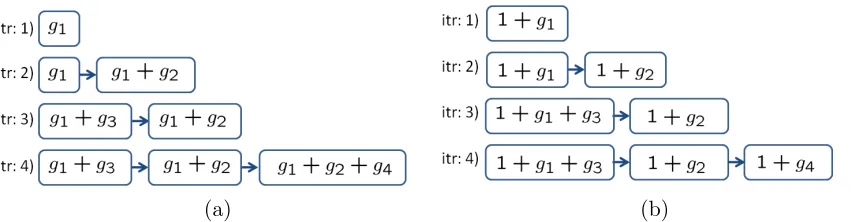
Figure 2: Illustration of the different configurations produced by identical steps of (a) last-stage and (b) multiplicative cascade learning.
6.2 Connections to the Previous Cascade Learning Literature
FCBoost supports a large variety of cascade structures. The cascade structure is defined by the generatorG of (28), since this determines the neutral predictorn(x), according to (56), and consequently how the cascade grows as boosting progresses. The two cascade predictors used in this work, last-stage and multiplicative, cover the two predominant cascade struc-tures in the literature. The first is theindependent stage (IS) structure, (Viola and Jones, 2001). In this structure stage predictors are designed independently,2 in the sense that the learning of fk starts from an empty predictor which is irrespective of the composition of the previous stages, fj, j < k. The second structure is the embedded stage (ES) structure where predictors of consecutive stages are related by
fk+1(x) =fk(x) +w(x),
and w(x) is a single or linear combination of weak learners (Xiao et al., 2003). Under this structure, each stage predictor contains the predictor of the previous stage, which is augmented with some weak learners.
The connection between these structures and the models proposed in this paper can be understood by considering the neutral predictors of the latter. For multiplicative cascades, it follows from (58) that
fm+1(x) = 1 +αg(x),
and there is no dependence between consecutive stages. Hence, multiplicative cascades have the IS structure. For last stage cascades, it follows from (57) that
fm+1(x) =fm(x) +αg(x).
If FCBoost always updates the last two stages, this produces a cascade with the ES struc-ture. Since FCBoost is free to update any stage, it can produce more general cascades, i.e., a superset of the set of cascades with the ES structure.
It is interesting that two predictors with the very similar generators of (32) and (37) produce very different cascade structures. This is illustrated in Figure 2, where we consider the cascades resulting from the following sequence of operations:
2. Note that the predictors are alwaysstatistically dependent, since the role ofhi+1is to classify examples
• iteration 1: start form an empty classifier, create first stage.
• iteration 2: add a new stage.
• iteration 3: update first stage.
• iteration 4: add a new stage.
Note that while the last-stage cascade of a) has substantial weak learner sharing across stages, this is not true for the multiplicative cascade of b), which is similar to the Viola and Jones cascade (Viola and Jones, 2001).
6.3 Properties
Beyond these connections to the literature, FCBoost has various interesting properties as a cascade boosting algorithm. First, its example weighing is very similar to that of adaboost (Freund and Schapire, 1997). A comparison of (5) and (15) shows that FCBoost reweights examples by how well they are classified by the current cascade. As in adaboost, this is measured by the classification margin, but now with respect to the cascade predictor,
F, (margin yF) rather than a simple predictor f (margin yf). Second, the weak learner selection rule of FCBoost is very similar to that of adaboost. While in (6) adaboost selects the weak learner g that maximizes
1
|St|
X
i
yiwig(xi),
in (52)-(53) FCBoost selects the stagek and weak learnerg that maximize
X
i
yiw(xi)bk(xi)
|St|
−ηy
s
iψk(xi)θk(xi)
|St−|
g(xi). (59)
A third interesting property of FCBoost is the complexity penalty (second term) of (59). From (44) and (50) this is, up to constants,
−yisγk(xi)efk(xi)C(Fk+1, xi)g(xi).
Given example xi and cascade stage k, all factors in this product have a meaningful in-terpretation. First, since ys
iγk(xi) is non-zero only for negative examples which have not been rejected by earlier cascade stages (j < k), it acts as a selector of the false-positives that reach stage k. Second, since fk(xi) measures how deeply xi penetrates the positive side of the stage k classification boundary, efk(xi) is large for the false-positives that stage k confidently assigns to the positive class. Third, since C(Fk+1, xi) is the complexity of processing xi by the stages beyond k, it measures how deeply xi penetrates the cascade, if not rejected by stage k. Finally, g(xi) is the label given to xi by weak learner g(x). Since only g(xi) can be negative, the product is maximized when g(xi) =−1, γk(xi) = 1 and fk(xi) and C(Fk+1, xi) are as large as possible. Hence, the best weak learner is that which, on average, declares as negatives the examples which 1) are false-positives of the earlier stages, 2) are most confidently accepted as false-positives by the current stage, and 3) penetrate the cascade most deeply beyond this stage. This is intuitive, in the sense that it encourages the selection of the weak learner that most contradicts the current cascade on its most costly mistakes.
In summary, FCBoost is a generalization of adaboost with similar example weighting, gating coefficients that guarantee consistency with the cascade structure, and a cost func-tion that accounts for classifier complexity. This encourages the selecfunc-tion of weak learners that correct the false-positives of greatest computational cost. It should be mentioned that while we have used adaboost to derive FCBoost, similar algorithms could be derived from other forms of boosting, e.g., logitboost, gentle boost (Friedman et al., 1998), KLBoost (Liu and Shum, 2003) or float boost (Li and Zhang, 2004). This would amount to replacing the exponential loss, (3), with other loss functions. While the resulting algorithms would be different, the fundamental properties (example reweighing, additive updates, gating coeffi-cients) would not. We next exploit this to develop a cost-sensitive extension of FCBoost.
6.4 Cost-Sensitive FCBoost
that weigh miss-detections more than false-positives, optimizing the cost-sensitive boundary directly. This usually outperforms threshold tuning.
In this work we adopt the cost sensitive risk of
RcE(f) = C
|St+| X
xi∈St+
e−yif(xi)+ 1−C |St−|
X
xi∈St−
e−yif(xi)
= X
xi∈St
ycie−yif(xi), (60)
whereC ∈[0,1] is a cost factor,
yic= C
|St+|I(yi = 1) +
1−C
|St−| I(yi =−1),
I(.) the indicator function, and the relative importance of positive vs. negative examples is determined by the ratio C
1−C (Viola and Jones, 2002). This leads to the cost-sensitive Lagrangian
Lc[F] =Rc
E[F] +RC[F]. (61)
A derivation similar to that of (14) can be used to show that
< δRcE[F], g >k=−
X
i
yiyciw(xi)bk(xi)g(xi), (62)
wherew(xi) =e−yiF(xi)andbk(xi) is given by (36) for last-stage and by (40) for multiplica-tive cascades. Finally, combining (61), (62), and (49),
<−δLc[F], g >k =
X
i
yiyciw(xi)bk(xi)−η
ys
iψk(xi)θk(xi)
|St−|
g(xi). (63)
The cost-sensitive version of FCBoost replaces (51) with (63) in (52)-(53) and L by Lc in (54).
6.5 Open Issues
One subtle difference between adaboost and FCBoost, with η= 0, is the feasible set of the underlying optimization problems. Rewriting the FCBoost problem of (13) as
minf RE[f]
s.t: f ∈ΩG,
(64)
where
ΩG={f|∃f1, ...fm∈G such that f(x) =Fm[f1, . . . , fm](x) ∀x}.
and comparing (64) to (2), the two problems differ in their feasible sets, span(G) for adaboost vs. ΩGfor FCBoost. Since any ˆf ∈span(G) is equivalent to a one-stage cascaded
predictor, it follows that ˆf ∈ΩGand
Hence, the feasible set of FCBoost is larger than that of adaboost, and FCBoost can, in principle, find detectors of lower risk. Hence, all generalization guarantees of adaboost hold, in principle, for cascades learned with FCBoost. There is, however, one significant difference. Since span(G) is a convex set, the optimization problem of (2) is convex wheneverRE(f) is a convex function of f. This is the case for the adaboost risk, and adaboost is thus guaranteed to converge to a global minimum. However, since ΩG can be a non-convex set,
no such guarantees exist for FCBoost. Hence, FCBoost can converge to a local minimum. We illustrate this with an example in Section 7.1. In general, the convexity of ΩGdepends on
the PC operatorFm and the set of weak learnersG. There is currently little understanding on what conditions are necessary to guarantee convexity.
7. Evaluation
In this section, we report on several experiments conducted to evaluate FCBoost. We start with a set of experiments designed to illustrate the properties of the algorithm. We then report results on its use to build face and pedestrian detectors with state-of-the-art performance in terms of detection accuracy and complexity. In all cases, the training set for face detection contained 4,500 faces (along with their flipped replicas) and 9,000 negative examples, of size 24×24 pixels, while pedestrian detection relied on a training set of 2,347 positive and 2,000 negatives examples, of size 72×30, from the Caltech Pedestrian data set (Doll´ar et al., 2012). All weak learners were decision-stumps on Haar wavelets (Viola and Jones, 2001).
7.1 Effect of η
We started by studying the impact of the Lagrange multiplier η, of (41), on the accuracy vs. complexity performance of FCBoost cascades. The test set consisted of 832 faces (along with their flipped replicas) and 1,664 negatives. All detectors were trained for 50 iterations. The unit computational cost was set to the cost of evaluating a new Haar feature. This resulted in a cost of 1
5 units for feature recycling, i.e., λ = 1
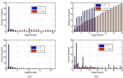
5 in (47). Figure 3 quantifies the structure of the cascades learned by FCBoost with η= 0 and η = 0.04: multiplicative in a) and last-stage in b). The top plots summarize the number of features assigned to each cascade stage, and those at the bottom the computational cost per stage. Note that since, from (57), the neutral predictor of the last-stage cascade is its last stage, each of the last-stage cascade stages benefits from the features evaluated in the previous stages. Hence, as shown in the top plot of Figure 3-b, the number of weak learners per stage is monotonically increasing. However, because most features are recycled, the cost is still dominated by the early stages, when η = 0. With respect to the impact of η, its is clear that, for both structures, a small η produces short cascades whose early stages contain many weak learners. On the other hand, a large η leads to much deeper cascades, and a more uniform distribution of weak learners and computation. This is sensible, since larger
0 5 10 15 20 0
10 20 30 40 50
Stage Number
Number of Features
η= 0
η= 0.04
0 5 10 15 20 25 30
0 10 20 30 40 50
Stage Number
Number of Features
η= 0
η= 0.04
0 5 10 15 20
0 10 20 30 40 50
Stage Number
Cost of Evaluation
η= 0
η= 0.04
0 5 10 15 20 25 30
0 5 10 15 20
Stage Number
Cost of Evaluation
η= 0
η= 0.04
(a) (b)
Figure 3: Number of features (top) and computational cost (bottom) per stage of an FC-Boost cascade: (a) multiplicative, (b) last-stage.
0.040 0.08 0.12 0.16 0.18 10
20 30 40 50
Error Rate
Cost of Evaluation
AdaBoost ChainBoost
Multiplicative
Last Stage
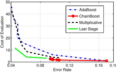
Figure 4: Computational cost vs. error rate of the detectors learned with adaboost, chain boost, and FCBoost with the last-stage and multiplicative structures.
adaboost FCBoost+last-stage FCBoost+multiplicative
Err. rate 4.03% 4.51% 4.15%
Eval. cost 50 11.74 42.54
Table 1: Performance comparison between adaboost and FCBoost, for η = 0.
(see Section 6.5). While the larger feasible set of FCBoost suggests that it should produce detectors of smaller risk than adaboost, this did not happen in our experiments.
Table 1 summarizes the error and cost of adaboost and the two FCBoost methods for
η= 0. Note that the adaboost detector has a slightly lower error. The weaker accuracy of the FCBoost detectors suggests that the latter does get trapped in local minima. This is, in fact, intuitive as the decision to add a cascade stage makes it impossible for the gradient descent procedure to revert back to a non-cascaded detector. By making such a decision, FCBoost can compromise the global optimality of its solution, if the global optimum is a non-cascaded detector. Interestingly, FCBoost sometimes decides to add stages even when
η = 0 (see Figure 3). As shown in Table 1, this leads to a slightly more error-prone but much more efficient detector than adaboost. In summary, even without pressure to minimize complexity (η= 0), FCBoost may trade-off error for complexity. This may be desirable or not, depending on the application. In the experiment of Table 1, FCBoost seems to make sensible choices. For the last-stage structure, it trades a small increase in error (0.48%) for a large decrease in computation (76.5%). For the multiplicative structure, it trades-off a very small increase in error (0.12%) for a moderate (16%) decrease in computation.
7.2 Cost-Sensitive FCBoost
0 0.2 0.4 0.6 0.8 0.84
0.88 0.92 0.96 1
False Positive Rate
Detection Rate
Last Stage Multiplicative
0.5 0.6 0.7 0.8 0.9 1 2
4 6 8 10 12
C
Evaluation Cost
Last Stage Multiplicative
(a) (b)
Figure 5: Performance of cascades learned with cost-sensitive FCBoost, using different cost factorsC. (a) ROC curves, (b) computational complexity.
cascades. In both cases, the leftmost (rightmost) point corresponds toC= 0.5 (C = 0.99). Figure 5 b) presents the equivalent plot for computational cost. Several observations can be made. First, as expected, larger cost factors C produce detectors of higher detection and higher false-positive rate. Second, they lead to cascades of higher complexity. This is intuitive since, for large cost factors, FCBoost aims for a high detection rate and is very conservative about rejecting examples. Hence, many negatives penetrate deep into the cascade, and computation increases. Third, comparing the curves of the last-stage and multiplicative cascades, the former again has better performance. In particular, last-stage cascades combine higher ROC curves in Figure 5 a) with lower computational cost in Figure 5 b).
7.3 Face and Pedestrian Detection
Over the last decade, there has been significant interest in the problem of real-time object detection from video streams. In particular, the sub-problems of face and pedestrian de-tection have been the focus of extensive research, due to the demand for face dede-tection in low-power consumer electronics (e.g., cameras or smart-phones) and pedestrian detection in intelligent vehicles. In this section, we compare the performance of FCBoost cascades with those learned by several state of the art methods in the face and pedestrian detection literatures.
We start with face detection, where cascaded detectors have become predominant, com-paring FCBoost to the method of Viola and Jones (VJ) (Viola and Jones, 2001), Wald boost (Sochman and Matas, 2005) and multi-exit (Pham et al., 2008). Since extensive re-sults on these and other methods are available on the MIT-CMU test set, all detectors were evaluated on this data set. The methods above have been shown to outperform a number of other cascade learning algorithms (Pham et al., 2008) and, to the best of our knowledge, hold the best results in this data set. In all cases, the target detection rate was set to
100 200 300 400 500 0.65
0.7 0.75 0.8 0.85 0.9 0.95
Number of False positives
Detection rate
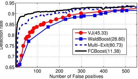
VJ(45.33) WaldBoost(28.80) Multi−Exit(80.73) FCBoost(11.38)
Figure 6: ROCs of various face detectors on MIT-CMU. The number in the legend is the av-erage evaluation cost, i.e., avav-erage number of features evaluated per sub-window.
and the popular strategy of setting the false positive rate to 50% and the detection rate to D
1 20
T . For FCBoost we used a last-stage cascade, since this structure achieved the best balance between accuracy and speed in the previous experiment. We did not attempt to optimizeη, simply usingη= 0.02. The cost factorC was initialized withC = 0.99. If after a boosting update the cascade did not meet the detection rate,C was increased to
Cnew =
Cold+ 1
2 . (65)
This placed more emphasis on avoiding misses than false positives, and was repeated until the updated cascade satisfied the rate constraint. The final value of C was used as the initial value for the next boosting update.
Figure 6 show the ROCs of all detectors. The average evaluation cost, i.e., average number of features evaluated per sub-window, is shown in the legend for each method. Note that the FCBoost cascade is simultaneously more accurate and faster than those of all other methods. For example, at 100 false positives, FCBoost has a detection rate of 91% as opposed to 88% for multi-exit, 83% for VJ, and 80% for Wald boost. With regards to computation, FCBoost is 7.1, 4, and 2.5 times faster than multi-exit, VJ, and Wald boost, respectively. Overall, when compared to the FCBoost cascade, the closest cascade in terms of detection rate (multi-exit, 3% drop) is significantly slower (7 times) and the closest cascade in terms of detection speed (Wald boost, 2.5 times slower) has a very poor detection rate (11% smaller).
10−3 10−2 10−1 100 101 102 .05
.10 .20 .30 .40 .50 .64 .80 1
false positives per image
miss rate
86% VJ(2.24) 38% HOG(4.18) 59% FtrMine(12.5) 77% Shapelet(19.60) 72% PoseInv 43% MultiFtr(13.89) 39% HikSvm(5.41) 50% LatSvm−V1(2.55) 28% LatSvm−V2(1.59) 30% ChnFtrs(0.85) 33% FPDW(0.15) 36% Pls(55.56) 23% HogLbp(16.13) 23% FCBoost(0.80) 36% MultiFtr+CSS(37.4) 16% MultiFtr+Motion(50)
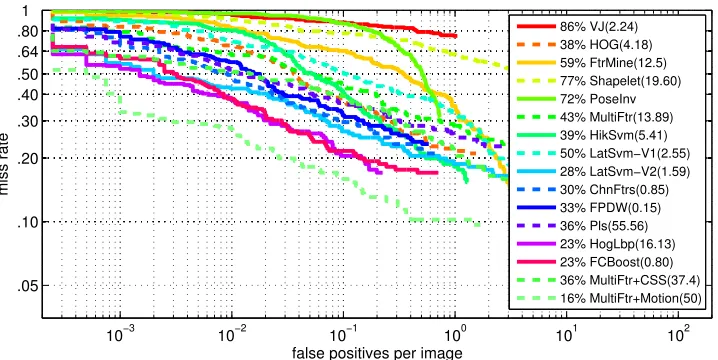
Figure 7: Accuracy curves and complexity of various pedestrian detectors on the Caltech data set. Legend: (left) miss rates at 0.1 FPPI, (right) average time, in seconds, required to process 480×640 frame.
architecture was as before, e.g., using Haar wavelet features and decision stumps as weak learners, the previously used values for parameters DT, and η, etc. When compared to the face detection experiments, the only difference is that the set of weak learners was replicated for each channel. At each iteration, FCBoost chose the best weak learner and the best channel to add to the cascade predictor. The performance of the FCBoost cascade was evaluated with the toolbox of (Doll´ar et al., 2012). Figure 7 compares its complexity and curve of miss-detection rate vs number of false positives per image (FPPI) to those of a number of recent pedestrian detectors. The comparison was restricted to the popular near scale-large setting, which evaluates the detection of pedestrians with more than 100 pixels in height. The numbers shown in the left of the legend summarize the detection performance by the miss rate at 0.1 FPPI. The numbers shown in the right indicated the average time, in seconds, required for processing a 480×640 video frame. Note that the evaluation is not restricted to fast detectors, including the most popular architectures for object detection in computer vision, such as the HOG detector (Dalal and Triggs, 2005) or the latent SVM (Felzenszwalb et al., 2010). For more information on the curves and other methods the reader is referred to Doll´ar et al. (2012).
comparable accuracy. In fact, only two detectors have been reported to achieve equivalent or lower miss rates. The Hog-Lbp detector (Wang et al., 2009) has the same miss rate (23% at 0.1 FPPI) but is 20 times slower. The MultiFtr+Motion (Walk et al., 2010) detector has a smaller miss rate of 16% (at 0.1 FPPI) but is 62 times slower (almost 1 minute per frame). The inclusion of this method in Figure 7 is somewhat unfair, since it is the only approach that exploits motion features. All other detectors, including the FCBoost cascade, operate on single-frames. We did not investigate the impact of adding motion features to FCBoost. Finally, it should be noted that the FCBoost cascade could be enhanced with various computational speed ups proposed in the design of the FPDW detector (Doll´ar et al., 2010). This is basically a fast version of the ChnFtrs detector, using several image processing speed-ups to reduce the time necessary to produce the image channels on which the classifier operates. These speed-ups lead to a significant increase in speed (0.15 vs 0.85 seconds) at a marginal cost in terms of detection accuracy (33% vs. 30% miss rate at 0.1 FPPI). Since these enhancements are due to image processing, not better cascade design, we have not considered them in our implementation. We would expect, however, to see similar computational gains in result of their application to the FCBoost cascade.
8. Conclusions
In this work we have addressed the problem of detector cascade learning by introducing the FCBoost algorithm. This algorithm optimizes a Lagrangian risk that accounts for both detector speed and accuracy with respect to a predictor that complies with the sequential decision making structure of the cascade architecture. By exploiting recursive properties of the latter, it was shown that many cascade predictors can be derived from generator functions, which are cascade predictors of two stages. Variants of FCBoost were derived for two members of this family, last-stage and multiplicative cascades, which were shown to generalize the popular independent and embedded stage cascade architectures. The concept of neutral predictors was exploited to integrate the search for cascade configuration into the boosting algorithm. In result, FCBoost can automatically determine 1) the number of cas-cade stages and 2) the number of weak learners per stage, by minimizing the Lagrangian risk. It was also shown that FCBoost generalizes adaboost, and is compatible with exist-ing cost-sensitive extensions of boostexist-ing. Hence, it can be used to learn cascades of high detection rate. Experimental evaluation has shown that the resulting cascades outperform current state-of-the-art methods in both detection accuracy and speed.
Acknowledgments
References
P. Bartlett and M. Traskin. Adaboost is consistent. Journal of Machine Learning Research, 8:2347–2368, December 2007.
L. Bourdev and J. Brandt. Robust object detection via soft cascade. In Proceedings of IEEE Conference on Computer Vision and Pattern Recognition, pages 236–243, 2005.
S. Brubaker, M. Mullin, and J. Rehg. On the design of cascades of boosted ensembles for face detection. International Journal of Computer Vision, 77:65–86, 2008.
G. Carneiro, B. Georgescu, S. Good, and D. Comaniciu. Detection and measurement of fetal anatomies from ultrasound images using a constrained probabilistic boosting tree.
IEEE Transactions on Medical Imaging, 27(9):1342 –1355, sept. 2008.
M. Collins, R. Schapire, and Y. Singer. Logistic regression, adaboost and Bregman distances.
Machine Learning, 48(1-3):253–285, 2002.
N. Dalal and B. Triggs. Histograms of oriented gradients for human detection. InProceedings of IEEE Conference on Computer Vision and Pattern Recognition, pages 886–893, 2005.
P. Doll´ar, Z. Tu, P. Perona, and S. Belongie. Integral channel features. In Proceedings of British Machine Vision Conference, 2009.
P. Doll´ar, S. Belongie, and P. Perona. The fastest pedestrian detector in the west. In
Proceedings of British Machine Vision Conference, 2010.
P. Doll´ar, C. Wojek, B. Schiele, and P. Perona. Pedestrian detection: An evaluation of the state of the art. IEEE Transactions on Pattern Analysis and Machine Intelligence, 34 (4):743–761, 2012.
S. Du, N. Zheng, Q. You, Y. Wu, M. Yuan, and J. Wu. Rotated Haar-like features for face detection with in-plane rotation. InProceedings of international conference on Interactive Technologies and Sociotechnical Systems, pages 128–137, 2006.
J. Duchi and Y. Singer. Boosting with structural sparsity. Proceedings of the International Conference on Machine Learning, pages 297–304, 2009.
M. Dundar and J. Bi. Joint optimization of cascaded classifiers for computer aided detection. In Proceedings of IEEE Conference on Computer Vision and Pattern Recognition, 2007.
P. Felzenszwalb, R. Girshick, D. McAllester, and D. Ramanan. Object detection with discriminatively trained part-based models. IEEE Transactions on Pattern Analysis and Machine Intelligence, 2010.
Y. Freund and R. Schapire. A decision-theoretic generalization of on-line learning and an application to boosting. Journal of Comp. and Sys. Science, 1997.
J. Friedman, T. Hastie, and R. Tibshirani. Additive logistic regression: a statistical view of boosting. Annals of Statistics, 28, 1998.
C. Lampert. An efficient divide-and-conquer cascade for nonlinear object detection. In
Proceedings of IEEE Conference on Computer Vision and Pattern Recognition, pages 1022 –1029, 2010.
C. Lampert, M. Blaschko, and T. Hofmann. Efficient subwindow search: A branch and bound framework for object localization. IEEE Transactions on Pattern Analysis and Machine Intelligence, pages 2129–2142, 2009.
L. Lefakis and F. Fleuret. Joint cascade optimization using a product of boosted classifiers. In Proceedings of the Neural Information Processing Systems Conference, 2010.
S. Li and Z. Zhang. Floatboost learning and statistical face detection. IEEE Transactions on Pattern Analysis and Machine Intelligence, 26(9):1112–1123, 2004.
R. Lienhart and J. Maydt. An extended set of Haar-like features for rapid object detection. In Proceedings of International Conference on Image Processing, pages I–900 – I–903 vol.1, 2002.
C. Liu and H. Shum. Kullback-Leibler boosting. In Proceedings of IEEE Conference on Computer Vision and Pattern Recognition, pages 587–594, 2003.
H. Luo. Optimization design of cascaded classifiers. InProceedings of IEEE Conference on Computer Vision and Pattern Recognition, pages 480–485, 2005.
H. Masnadi-Shirazi and N. Vasconcelos. High detection-rate cascades for real-time object detection. In Proceedings of International Conference on Computer Vision, volume 2, pages 1–6, 2007.
H. Masnadi-Shirazi and N. Vasconcelos. Cost-sensitive boosting. IEEE Transactions on Pattern Analysis and Machine Intelligence, 99, 2010.
L. Mason, J. Baxter, P. Bartlett, and M. Frean. Functional gradient techniques for com-bining hypotheses. Advances in Large Margin Classifiers, pages 1221–246, 2000.
D. Mease and A. Wyner. Evidence contrary to the statistical view of boosting. Journal of Machine Learning Research, 9:131–156, 2008.
C. Messom and A. Barczak. Fast and efficient rotated haar-like features using rotated inte-gral images. InProceedings of the Australasian Conference on Robotics and Automation, 2006.
M. Pham and T. Cham. Fast training and selection of Haar features using statistics in boosting-based face detection. InProceedings of IEEE International Conference on Com-puter Vision, pages 1–7, 2007.
M. Pham, V. Hoang, and T. Cham. Detection with multi-exit asymmetric boosting. In