Efficient State-Space Inference of Periodic Latent Force
Models
Steven Reece [email protected]
Department of Engineering Science University of Oxford
Parks Road
Oxford OX1 3PJ, UK
Siddhartha Ghosh [email protected]
Alex Rogers [email protected]
Electronics and Computer Science University of Southampton Southampton SO17 1BJ, UK
Stephen Roberts [email protected]
Department of Engineering Science University of Oxford
Parks Road
Oxford OX1 3PJ, UK
Nicholas R. Jennings [email protected]
Electronics and Computer Science University of Southampton Southampton SO17 1BJ, UK and
Department of Computing and Information Technology King Abdulaziz University
Saudi Arabia
Editor:Neil Lawrence
Abstract
efficiently using state-space methods which encode the linear dynamic systems via LFMs. Further, we show that state estimates obtained using periodic latent force models can re-duce the root mean squared error to 17% of that from non-periodic models and 27% of the nearest rival approach which is the resonator model (S¨arkk¨a et al., 2012; Hartikainen et al., 2012).
Keywords: latent force models, Gaussian processes, Kalman filter, kernel principle com-ponent analysis, queueing theory
1. Introduction
Latent force models (LFMs) have received considerable interest in the machine learning community as they combine underlying physical knowledge of a system with data driven models expressed as Bayesian non-parametric Gaussian process (GP) priors (see, for exam-ple, Alvarez et al., 2009; Hartikainen and S¨arkk¨a, 2010). In more detail, the physical process that generates the data is typically represented by one or more differential equations. These differential equations can then be accommodated within covariance functions along with the data driven priors. Doing so allows inferences to be drawn in regimes where data may be sparse or absent, where a purely data driven model will typically perform poorly. To date, such models have been applied in areas such as computational biology and understanding motion patterns (Alvarez et al., 2009, 2010).
Despite growing interest in LFMs, their real world applicability has been limited as in-ference using LFMs expressed directly through covariance functions can be computationally prohibitive on large data sets. It is well known that regression with GPs imposes high com-putational cost which scales as O(N3T3) during training, where N is the dimension of the data observed at each time point and T is the number of time points. However, it has also been shown that training LFMs using state-space methods can be considerably less com-putationally demanding (Rasmussen and Williams, 2006; Hartikainen and S¨arkk¨a, 2010) as state-space methods scale as O(N3T). It is this computational saving that motivates the state-space approach to LFM inference in this paper.
The state-space approach to LFM inference advocated by Hartikainen and S¨arkk¨a (2010, 2011) augments the state vector so that Mat´ern and squared-exponential priors can be accommodated (although only approximately in the case of the squared-exponential). All the information encoded within the GP prior (that is, process smoothness, stationarity etc) is fully captured within their state-space representation. However, their approach assumes that the LFM kernel’s inverse power spectrum can be represented by a power series in the frequency domain. Unfortunately, this requirement severely inhibits the applicability of their approach and, consequently, only a small repertoire of GP priors have been investigated within LFMs to date, namely, squared-exponential and Mat´ern kernels. Specifically, the state-space approach advocated by Hartikainen and S¨arkk¨a (2010) does not accommodate periodic kernels as we shall demonstrate in this paper. This is a key limitation as periodicity is common in many physical processes as we shall demonstrate in our empirical evaluation. Expressing our prior knowledge of the periodicity, as a GP prior, within the state-space approach is the key challenge problem addressed in this paper.
inferred using Bayesian methods or maximum likelihood and thus we circumvent the need to set any of these parameters by hand. Further, to accommodate periodic and quasi-periodic models within LFMs we develop a novel state-space approach to inference. In particu-lar, we propose to represent periodic and quasi-periodic driving forces, which are assumed smooth, by linear basis models (LBMs) with eigenfunction basis functions derived using kernel principal component analysis (KPCA) in the temporal domain. These basis models, although parametric in form, are optimized so that their generative properties accurately approximate the driving force kernel. We will show that efficient inference can then be performed using a state-space approach by augmenting the state with additional variables which sparsely represent the periodic latent forces.
Our LBM approach to accommodating periodic kernels is inspired by the resonator model(S¨arkk¨a et al., 2012; Hartikainen et al., 2012) in which the periodic process is modelled as a superposition of resonators, each of which can be represented within the state-vector. Unfortunately, the resonator model, in its current form, does not encode all the underlying GP prior information of the periodic process as the resonator is not tailored to accommo-date all the prior information encoded via the covariance function (see Section 4 for more detail). An alternative approach to modelling stationary kernels, including periodic kernels, is sparse spectrum Gaussian process regression (SSGPR) of L´azaro-Gredilla et al. (2010). This approach is similar in spirit to the resonator model in that it encodes stationary GP priors via basis functions (sinusoidal functions, in this case). However, unlike the resonator model, the SSGPR is able to encode the GP prior by reinterpreting the spectral density of a stationary GP kernel as a probability density function over frequency space. This pdf is then sampled using Monte Carlo to yield the frequencies of the sinusoidal basis func-tions. Unfortunately, this stochastic approach can often provide a poor approximation to the covariance function (see Section 5 for more detail).
We shall develop a LBM which captures all the information encoded within the GP prior and demonstrate its superior accuracy over the resonator model and the SSGPR. We shall also establish the close link between the resonator basis and the eigenfunction basis used in our approach and consequently, derive a novel method for tailoring the resonator basis to accommodate all the information encoded within the covariance function.
application and regular measurements are available whereas the thermal application requires long term predictions (a day ahead) during which no measurements are available.
In more detail, telephone call centre managers are concerned with staffing and specifi-cally, assigning the appropriate number of agents to guarantee that the customers’ queueing time does not prohibit sales (Feigin et al., 2006). Although there is significant literature on attempts to accurately model the dynamics of queues, it has failed to offer a method for inferring the highly quasi-periodic arrival rates from sparse measurements of the queue lengths (Wang et al., 1996). Determining such arrival rates is key to predicting queue lengths, and hence customer waiting times. These predictions help the call centre manager to plan staffing throughout the day to ensure an acceptable customer waiting time. We will demonstrate that our approach to modelling LFMs is capable of inferring these unknown arrival rates. Furthermore, although the dynamic system in this application is nonlinear and the arrival rate is quasi-periodic, it is still Markovian and, consequently, a state-space approach to inference is ideally suited to this application.
Energy saving in homes is a key issue as governments aim to reduce the carbon footprint of their countries. A significant amount of energy is expended in heating homes and home owners need to be encouraged to reduce their energy consumption and carbon emissions incurred through home heating (MacKay, 2009; DECC, 2009). Consequently, we apply our approach to the estimation and prediction of internal temperatures using thermal models of home heating systems. Our approach allows us to make day ahead predictions of the energy usage, which can then be fed back to the householder in real-time so that they can take appropriate mitigating actions to reduce their energy consumption. Home heating systems typically consist of a thermostat with a set-point that controls the activations of a gas or electrical boiler to ensure that the internal temperature follows the set-point. Although there is significant literature on attempts to accurately model the thermal dynamics of buildings, it has failed to take into account the daily human behaviours within their homes, which can have a significant impact on the energy signatures obtained from similar homes (Bacher and Madsen, 2011). For instance, during cold periods, a householder may deploy an additional heater or, in hot periods, open a window. Furthermore, the thermal dynamics of real homes are more complex in reality than existing thermal models suggest; sunlight through windows contributes to extra heat while open windows cause heat loss. Residual heat can also be retained by thermal blocks such as walls and ceilings that then re-radiate heat. Crucially, many of these heat sources are periodic in nature. For instance, an addi-tional heater may be switched on every night during cold periods, whilst the diurnal sun cycle will contribute additional heat during the day. We will demonstrate that our approach is capable of inferring these unknown periodic heat sources. Again, the dynamic system in this application is linear and Markovian and, consequently, a state-space approach to inference is again ideally suited to this problem.
In undertaking this work, we advance the state of the art in the following ways:
• We offer the only principled approach to incorporating all Gaussian process prior models within a state-space approach to inference with LFMs.1
• We are the first to demonstrate that the eigenfunction model of Gaussian process priors out-performs an alternative approach to modelling periodic Gaussian process priors; namely, the sparse spectrum Gaussian process regression (SSGPR) approach developed by L´azaro-Gredilla et al. (2010).
• We demonstrate, for the first time, the close link between the eigenfunction model and the resonator model (S¨arkk¨a et al., 2012; Hartikainen et al., 2012; Solin and S¨arkk¨a, 2013). Consequently, we offer a novel mechanism for incorporating all information encoded within the latent force covariance function into the resonator model.
• We propose the only approach that is able to incorporate all types of periodic Gaussian process priors within a state-space approach to LFM inference. These priors include stationary periodic, non-stationary periodic and quasi-periodic covariance functions.
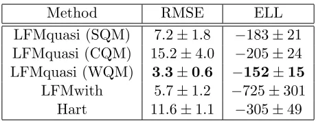
• We are the first to apply LFMs to queueing theory, specifically to the modelling of queue arrival rates. Through empirical evaluation, we show that for tracking the customer queue lengths in the call centre application, the RMSE of our approach using a quasi-periodic kernel model of the arrival rate can be 17% of that using the same approach with a non-periodic kernel model.
• We are the first to apply LFMs to the modelling of thermal dynamics within real homes, specifically to unknown physical thermal processes. We show that for day ahead predictions of temperature in homes, the RMSE of our approach is 45% of that obtained using the resonator model (Solin and S¨arkk¨a, 2013) when the latent forces exhibit quasi-periodic behaviour.
2. A Review of Gaussian Process Priors and Inference
A Gaussian process (GP) is often thought of as a Gaussian distribution over functions (Rasmussen and Williams, 2006). A GP is fully described by its mean function, µ, and
covariance function,K. A draw, f, from a GP is traditionally written as
f ∼ GP(µ, K).
The value of the function, f, at inputs X is denoted f(X). Similarly, the value of the mean function and covariance function at these inputs are denoted µ(X) and K(X, X), respectively. The meaning of a GP becomes clear when we consider that, for any finite set of inputs,X,f(X) is a draw from a multi-variate Gaussian, f(X)∼ N(µ(X), K(X, X)).
Suppose we have a set of training data
D={(x1, y1), . . . ,(xn, yn)}, (1) drawn from a function, f with
yi =f(xi) +i,
wherei is a zero-mean Gaussian random variable with varianceσ2. For convenience both inputs and outputs are aggregated into setsX={x1, . . . , xn}andY ={y1, . . . , yn}, respec-tively. The GP estimates the value of the function f at test inputs X∗ ={x∗1, . . . , x∗m}. The basic GP regression equations are given by
¯
f∗ =µ(X∗) +K(X∗, X)[K(X, X) +σ2I]−1(Y −µ(X)), (2)
Var(f∗) =K(X∗, X∗)−K(X∗, X)[K(X, X) +σ2I]−1K(X∗, X)T, (3)
where I is the identity matrix, ¯f∗ is the posterior mean function at X∗ and Var(f∗) is the
posterior covariance (Rasmussen and Williams, 2006). The inversion operation present in Equations (2) and (3) is the source of the cubic computational complexity reported in the previous section.
The matrix K(X, X) is the covariance of the Gaussian prior distribution over f(X). The covariance matrix has elements
K(xi, xj) = Cov(f(xi), f(xj)),
where the term K(X∗, X) is the covariance between the function, f, evaluated at the test
inputsX∗ and the training inputsX. The functionK is alternatively called the kernelor
The GP parameters θ (which includes σ and hyperparameters associated with the co-variance function) can be inferred from the data through Bayes’ rule
p(θ|Y, X) = p(Y |X, θ)
p(Y |X) p(θ).
The parameters are usually given a vague prior distribution p(θ). In this paper, since our applications in Sections 8 and 9 exploit large data sets, we use maximum likelihood to infer the parameters and identify the assumed unique value for θ which maximizes p(Y |
X, θ). This approach is preferred over full Bayesian marginalisation (Bishop, 1999) as the preponderance of data in the applications we consider produces very tight posterior distributions over the parameters.
When the Gaussian process models a time series then the input variables, X, are values of time. We shall assume that increasing input indices correspond to sequential time stamps,
x1 ≤x2 ≤. . .≤xn−1 ≤xn. We are at liberty to deploy GP inference using Equations (2)
and (3) to either interpolate the function f(x∗) at x∗ when x1 < x∗ < xn or extrapolate
f(x∗) when either x∗ < x1 or x∗ > xn. When measurements are obtained sequentially, extrapolation forward in time is termed prediction and the inference of f(x∗) is termed
filtering. Interpolation with sequential measurements is termed smoothing. Although both smoothing and filtering approaches have been developed for Gaussian process regression (Hartikainen and S¨arkk¨a, 2010), we shall be concerned with filtering only. However, the eigenfunction models for periodic Gaussian processes developed in this paper can also be used for smoothing.
In the next section we review the latent force model (LFM) which is a principled ap-proach to incorporating solutions to differential equations within Gaussian process inference methods.
3. Latent Force Models
In this section we present a brief introduction to latent force models and describe their practical limitations. Specifically, we consider dynamic processes which can be described by a set of E coupled, stochastic, linear, first order differential equations
dzq(t)
dt =
E
X
e=1
Fe,qze(t) + R
X
r=1
Lr,qur(t),
where q and e index each variable z, R is the number of latent forces and r indexes each latent force u, and L and F are coefficients of the system. For example, in our home heating application (described in detail in Section 9),z1(t) models the internal temperature
of a home,z2(t) the ambient temperature immediately outside the home,u1(t) is the heater
output from a known proportional controller andu2(t) is an unknown residual force. In this
application, we assumeu2(t) is periodic as it is used to model solar warming, some habitual
human behaviour and the thermal lags in the heating system. The resulting differential equations can be written as
dz(t)
where u(t) is a vector of R independent driving forces (also called the latent forces). We distinguish non-periodic latent forces, np, and periodic latent forces, p, as they will be modelled differently in our approach. Non-periodic forces will be modelled using the existing approach advocated in Hartikainen and S¨arkk¨a (2010), which is reviewed in Section 4, and periodic forces will be modelled using our novel linear basis approach presented in Section 5. In Equation (4) theE×E matrix Fand theE×R matrixL are non-random coefficients that link the latent forces to the dynamic processes. Although we deal with first order differential equations only, all higher order differential equations can be converted to a set of coupled first order equations (Hartikainen and S¨arkk¨a, 2010).
Following Alvarez et al. (2009) and Hartikainen and S¨arkk¨a (2010, 2011) we assume that the latent forces, u, are independent draws from Gaussian processes, ui ∼ GP(0, Ki) whereKi is the GP covariance function (Rasmussen and Williams, 2006) for forceui. Con-sequently, the covariance for z at any timest and t0 can be evaluated as
E[(z(t)−¯z(t))(z(t0)−¯z(t0))T] =Φ(t0, t)P0zΦ(t0, t0)T + Γ(t0, t, t0), (5)
whereΦ(t0, t) denotes the matrix exponential,Φ(t0, t) = exp(F(t−t0)) expressed in Alvarez
et al. (2009), ¯z(t) =E[z(t)] and2 Γ(t0, t, t0) =
Z t
t0
Z t0
t0
Φ(s, t)LK(s, s0)LTΦ(s0, t0)T ds ds0.
P0z is the state covariance at time t0, P0z =E[(z(t0)−¯z(t0))(z(t0)−¯z(t0))T] and K(s, s0)
is the diagonal matrix K(s, s0) = diag(K1(s, s0), . . . , KR(s, s0)). Since z(t) is a vector and defined for any timestandt0thenE[(z(t)−¯z(t))(z(t0)−¯z(t0))T] is a multi-output Gaussian process covariance function. A kernel for covariances between the target,z, and the latent forces,u, can also be derived. Inference with these kernels is then undertaken directly using Equations (2) and (3).
Unfortunately, a na¨ıve implementation of LFM inference using Equations (2) and (3) and covariance functions derived using Equation (5) can be computationally prohibitive. As we have already pointed out, this approach can be computationally expensive due to the need to invert prohibitively large covariance matrices. To mitigate computational intensive matrix inversion in the GP equations, various sparse solutions have been proposed (see, for example, Williams and Seeger, 2001; Snelson and Ghahramani, 2006; L´azaro-Gredilla et al., 2010) and an early review of some of these methods is presented in Qui˜nonero Candela and Rasmussen (2005). Unfortunately, the spectral decomposition approach of L´azaro-Gredilla et al. (2010) is sub-optimal in that it randomly assigns the components of a sparse spectral representation and this limitation is explored in detail in Section 5. The Nystr¨om method for approximating eigenfunctions is used in Williams and Seeger (2001) to derive a sparse approximation for the kernel which can then be used to improve the computational efficiency of the GP inference Equations (2) and (3). Unfortunately, this approximate kernel is not used consistently throughout the GP equations and this can lead incorrectly to negative predicted variances.
The pseudo-input approach (also calledinducing inputs,Snelson and Ghahramani, 2006; Qui˜nonero Candela and Rasmussen, 2005) is a successful method for reducing the number
of input samples used within GP inference without significantly losing information en-coded within the full data set. In essence, densely packed samples are summarized around sparsely distributed inducing points. Pseudo-inputs have been successfully deployed within sparse approximations of dependent output Gaussian processes (Alvarez and Lawrence, 2008, 2011). Pseudo-inputs have recently been introduced to GP time-series inference and applied to problems which exploit differential equations of the physical process via the la-tent force model (Alvarez et al., 2011). In Alvarez et al. (2011) the lala-tent force is expressed at pseudo-inputs and then convolved with a smooth function to interpolate between the pseudo-inputs. However, although inducing inputs can reduce the sampling rate and sum-marize local information, they still have to be liberally distributed over the entire time se-quence. We may assume, for simplicity, the pseudo-inputs are evenly spread over time and, therefore, the number of pseudo-inputs, P, would have to increase linearly with the num-ber of observations (although with a rate considerably lower than the observation sampling rate). Unfortunately, the computational complexity of GP inference with pseudo-inputs is
O(T P2) where T is the number of observations (Alvarez and Lawrence, 2008). Thus, al-though pseudo-inputs are able to improve the efficiency of GP inference to some extent, for time series analysis their computational cost is still cubic in the number of measurements and this can be computationally prohibitive.
In the next section we describe a state-space reformulation of the LFM. The state-space approach has the advantage that it has a computational complexity for inferring the target process, z, which is O(T) but at the expense of representing the target process with extra
state variables.
4. State-Space Approaches to Latent Force Models
In this section we review the current state-space approach to inference with LFMs (Har-tikainen and S¨arkk¨a, 2010) and show how some covariance functions can be represented exactly in state-space. Unfortunately, we shall also demonstrate that periodic kernels can-not be incorporated into LFMs using the approach advocated by Hartikainen and S¨arkk¨a (2010). To address this key issue, we will then propose to approximate a periodic covari-ance function with a sparse linear basis model. This will allow us to represent periodic behaviour within a LFM efficiently and also incorporate information encoded within the periodic kernel prior. Our work is inspired by, and can be seen as, an extension of the res-onator model (S¨arkk¨a et al., 2012; Hartikainen et al., 2012), which is an alternative linear basis model that allows periodic processes to be modelled within the state-space approach. Our LBM approach, described in Section 5, builds on the resonator model and extends it by incorporating the prior information encoded within the latent force covariance function. When the target processes, zas per Equation (4), can be expressed in Markov form, we can avoid the need to invert large covariance matrices and also avoid the need to evaluate Equation (5) over long time intervals, [t0, t], by using the more efficient state-space inference
approach advocated by Hartikainen and S¨arkk¨a (2010) and in this paper. The temporal computational complexity of the state-space approach is O(T) as we integrate over short time intervals, [t0, t], and then reconstruct long term integrations by conflating the local
over long intervals, [t0, t], and then regress using Equations (2) and (3). Both approaches are
mathematically equivalent in that they produce identical inferences when they are applied to the same differential model, latent force covariance functions and data.
The Kalman filter is a state-space tool for time series estimation with Gaussian pro-cesses (Kalman et al., 1960). The Kalman smootheris also available for interpolation with sequential data. The Kalman filter is a state-space inference tool which summarizes all information about the process, f, at time x via astate description. The advantage of the Kalman filter is that any process f∗ at any future timex∗ can be inferred from the current
state without any need to refer to the process history. The state at any timex is captured by a finite set of Gaussian distributedstate variables,U, and we assume thatf is a linear function of the state variables. In Hartikainen and S¨arkk¨a (2010) the state variables corre-sponding to each latent force f are the function f and its derivatives. In our approach the state variables corresponding to each periodic latent force will be the eigenfunctions of the periodic covariance function. The key advantage of the Kalman filter is that its computa-tional complexity is linear in the amount of data from a single output time-series. Contrast this with the standard Gaussian process approach, as per Equations (2) and (3), which require the inversion of a covariance matrix and thus, have a computational complexity which is cubic in the amount of data.3
To illustrate the state-space approach consider a single non-periodic latent force, ur(t), indexed byr, in Equation (4). We assume that this force is drawn from a Gaussian process thus
ur∼ GP(0, Kr),
whereKr is a stationary kernel. In Hartikainen and S¨arkk¨a (2010) the authors demonstrate that a large range of stationary Gaussian process kernels,Kr, representing the latent force prior can be transformed into multivariate linear time-invariant (LTI) stochastic differential equations of the form
dUr(t)
dt =Fr Ur(t) +Wr ωr(t), (6)
whereUr(t) = (ur(t), dudtr(t), · · ·,d
pr−1u
r(t)
dtpr−1 )T and
Fr =
0 1
. .. . ..
0 1
−c0r · · · −crpr−2 −cprr−1
, Wr=
0 .. . 0 1
, (7)
where c are coefficients which can be set using spectral analysis of the kernel as per Har-tikainen and S¨arkk¨a (2010). The force, ur(t), can be recovered from Ur(t) using the indi-cator vector∆r= (1,0, . . . ,0) where
ur(t) =∆rUr(t).
By choosing the coefficientsc0r, . . . , cprr−1 in Equation (7), the spectral density of the white noise process ωr(t) in Equation (6) and the dimensionality pr of Ur(t) appropriately, the covariance ofur(t), corresponding to the dynamic model, can be chosen to correspond to the GP prior Kr. The differential equations expressed in Equation (6) can then be integrated into the LFM to form the augmented dynamic model expressed later in Equation (12). The coefficients c0r, . . . , cpr−1
r are found by initially taking the Fourier transform of both sides of Equation (6). The coefficients can then be expressed in terms of the spectral density of the latent force kernel, Kr, provided that its spectral density, Sr($), can be written as a rational function of $2 thus
Sr($) =
(constant)
(polynomial in$2) . (8)
The inverse power spectrum is then approximated by a polynomial series from which the transfer function of an equivalent stable Markov process for the kernel can be inferred along with the corresponding spectral density of the white noise process. The stochastic differential equation coefficients are then calculated from the transfer function. For example, for the first-order Mat´ern kernel given by
Kr(t, t0) =σ2rexp
−|t−t
0|
lr
, (9)
with output scaleσr and input scalelr,ur∼ GP(0, Kr) can be represented by Equation (6) withUr(t) =ur,Wr= 1 and
Fr=−1/lr. (10)
The spectral density, λr, of the white noise process,ωr, is
λr=
2σr2√π lr Γ(0.5)
, (11)
and Γ is the Gamma function (Hartikainen and S¨arkk¨a, 2010).
Now, by augmenting the state vector, z in Equation (4), with the non-periodic forces
Ur(t) and their derivatives, Hartikainen and S¨arkk¨a (2011) demonstrate that the dynamic equation can be rewritten as a joint stochastic differential model thus
dza(t)
dt =Fa za(t) +Laωa(t), (12)
where
za(t) = (z(t), U1(t), . . . , UR(t))T,
Fa =
F LS1∆1 . . . LSR∆R
0 F1 . . . 0
.. .
0 0 . . . FR
Ris the number of latent forces,Sr= (0, . . . ,1, . . . ,0) is the indicator vector which extracts therth column ofL corresponding to therth force, ur, and ωa(t) is the appropriate scalar process noise
ωa(t) = (0, ω1(t), . . . , ωR)T, (13)
La = blockdiag(0, W1, . . . ,WR). (14)
These differential equations have the solution
za(t) =Φ(t0, t)za(t0) +qa(t0, t),
where, again,Φ(t0, t) denotes the matrix exponential, Φ(t0, t) = exp(Fa(t−t0)) expressed
in Alvarez et al. (2009). The process noise vector, qa(t0, t), is required to
accommo-date the Mat´ern or SE latent forces within the discrete time dynamic model, qa(t0, t) ∼ N(0,Qa(t0, t)) where
Qa(t0, t) =
Z t
t0
Φ(s, t)LaΛaLTaΦ(s, t)Tds,
and Λa is a diagonal matrix
Λa= diag(0, λ1, . . . , λR), (15)
whereλr is the spectral density of the white noise process corresponding to the Mat´ern or SE process,Kr (Hartikainen and S¨arkk¨a, 2010).
We now briefly describe the reasons why this spectral analysis approach advocated by Hartikainen and S¨arkk¨a (2010, 2011) cannot be immediately applied to periodic kernels. For illustrative purposes we shall investigate the commonly used squared-exponential periodic kernel expressed as
KSE(t, t0) = exp
−
sinπ(tD−t0)2
l2
, (16)
−20 0 20 0
2 4 6 8 10 12
Recip. Power Spectrum
Frequency
True Polynomial
0 5 10
−1 0 1 2 3 4 5 6 7 8
Order
Polynomial Coefficient for 1/S
0 5 10
0 0.2 0.4 0.6 0.8 1
Input
Covariance
True Recovered
Figure 1: Spectral analysis of a periodic covariance function. The left panel shows inverse power spectrum for a periodic squared-exponential kernel (thin line) and its poly-nomial approximation (thick line). The central panel shows the coefficients of the polynomial approximation. The right panel shows the true covariance function (crossed line) and its approximation (solid line) recovered from the polynomial representation of the inverse power spectrum.
So, it is not possible to formulate all periodic latent forces via Equation (6). However, by approximating the latent force as a linear sum of basis functions, such that each basis function, φ, can be formulated via Equation (6) as
ur(t) =
X
j
arjφj(t), (17)
then it is possible to represent the periodic latent force within the KF. In essence, the latent force, ur, is decomposed into a weighted sum of basis latent forces, {φj}, such that each φsatisfies Equation (6). This is the approach of S¨arkk¨a et al. (2012) for representing both stationary and quasi-periodic latent forces via their resonator model. In Hartikainen et al. (2012), the resonator,φr, is chosen to be a Fourier basis,φr(t) = cos(frt) orφr(t) = sin(frt). The resonator can be represented by Equation (6) as a state comprising the instantaneous resonator value,φr(t), and its derivative, ˙φr(t) thus,Ur(t) = (φr(t), φ˙r(t))T. The corresponding SDE has Fr = [0 1 ; −fr2 0] and Wr = 0. The Fourier basis is particularly useful for modelling stationary covariance functions.
In Hartikainen et al. (2012) quasi-periodic latent forces were implemented as a super-position
u(t) =X j
of resonators, ψ, of the form
d2ψj(t)
dt2 =−(2πfj(t)) 2ψ
j(t) +ωj(t), (19)
where ω is a white noise component. Crucially, the resonator frequencies, f, are time variant and this supports non-stationary and quasi-periodic forces. This model is very flexible and both periodic and quasi-periodic processes can be expressed using the resonator model (as detailed in Appendix B). However, currently no mechanism has been proposed to incorporate prior information encoded in periodic GP kernels within the resonator model. Further, inferring the parameters and the frequency profiles,f(t), for each resonator can be prohibitively computationally expensive (as we demonstrate in Appendix B). Despite these shortcomings there is a very close connection between the resonator model for periodic latent forces and the eigenfunction approach proposed in this paper. This connection is explored in detail in Appendix B in which we assert that the eigenfunction basis is an instance of the resonator basis for perfectly periodic covariance functions. We subsequently demonstrate how the eigenfunction approach can both inform the resonator model of the GP prior and also simplify the inference of the resonator model parameters including the frequency profile. Further, we show that the optimal minimum mean-square resonator model is an alternative way of representing the corresponding eigenfunction basis within the Kalman filter.
In the original implementation of the resonator model (S¨arkk¨a et al., 2012) the model parameters were set by hand. Recently, a new variation of the resonator model has been proposed in which the most likely model parameters are learned from the data (Solin and S¨arkk¨a, 2013). In this version the resonator is the solution of the time invariant second order differential equation
d2ψj(t)
dt2 =Ajψj(t) +Bj dψj(t)
dt +ωj(t), (20)
where A and B are constant coefficients. We note that this variation of the resonator model is a special case of the original resonator model with a frequency profile fj(t) =
i
2π
q
Aj +Bjψj1(t)dψdtj(t) in Equation (19). To model quasi-periodic processes Equation (20) comprises a decay term via the first derivative of the resonator function. This new model is computationally efficient as it imposes constant coefficients unlike the original resonator model in S¨arkk¨a et al. (2012). However, the computational efficiency of the model in Equa-tion (20), gained by losing the requirement to infer a frequency profile for each resonator, is at the expense of the model’s flexibility. We compare the resonator model in Equation (20) with our eigenfunction approach on a real world application in Section 9.
In preparation for the approach advocated in this paper, in which we also represent the periodic kernel via a linear basis model, the following section compares the two key alter-native approaches to directly inferring linear basis models from Gaussian Process kernels, namely the sparse spectrum Gaussian process regression (SSGPR, L´azaro-Gredilla et al., 2010) and kernel principal component analysis (Sch¨olkopf and M¨uller, 1998).
5. Representing Periodic Latent Forces with Linear Basis Models
kernels so that they can be accommodated within a state-space formulation of the LFM. Linear basis models (LBMs) have a long history in machine learning. In particular, special cases of them include kernel density estimators (Parzen, 1962) and the Relevance Vector Machine (Tipping, 2001). There are two key advantages to representing periodic kernels using a sparse basis model: firstly, they can approximate the kernel using a weighted sum over a finite set of functions. As we will see, for relatively smooth kernels the number of basis functions can be small. The second advantage, as we will show in Section 7, is that the LBM representation is amenable to inference using computationally efficient state-space methods. We exploit the Nystr¨om approximation as opposed to other sparse approximations (such as the sparse spectrum Gaussian process regression method of L´azaro-Gredilla et al., 2010) as, we will see, the eigenfunctions of the kernel form the most efficient basis for the corresponding driving forces. This approximation will accommodate both the prior information about the driving forces (encoded in the kernel) within a state-space approach and also provide a means to learn these driving forces from data using iterative state-space methods. Approximating Gaussian process priors via the Nystr¨om method is not new (see, for example, Williams and Seeger, 2001). However, using this to accommodate periodic and quasi-periodic latent forces within LFMs is novel.
In order to develop our LBM for latent forces we shall first investigate current approaches to sparse representations of stationary covariance functions and then demonstrate that one of these approaches, namely the eigenfunction approach, generalizes to non-stationary covariance functions. Bochner’s theorem asserts that all stationary covariance functions can be expressed as the Fourier transform of their corresponding spectral densities (where the spectral density exists. See, for example, Rasmussen and Williams, 2006). Furthermore, in the stationary case, the Fourier basis is the eigenfunctions of the covariance function. There has been a long history of research into the spectral analysis of stationary Gaussian process kernels (see, for example, Bengio et al., 2004). However, only recently has the Fourier basis been investigated in the context of latent force models. To date, two approaches have been proposed to incorporate knowledge of all stationary kernels, including periodic kernels, within the linear basis representation via spectral analysis: the SSGPR (L´azaro-Gredilla et al., 2010) and the KPCA (Drineas and Mahoney, 2005) method. The key advantage of these approaches is that the basis frequencies can be calculated from the prior latent force kernel. These approaches are described and compared next.
The SSGPR (L´azaro-Gredilla et al., 2010) approach reinterprets the spectral density of a stationary GP kernel as the probability density function over frequency space. This pdf is then sampled using Monte Carlo to yield the frequencies of the sinusoidal basis functions of the LBM.4 The advantage of this approach is that a sparse set of sinusoidal basis functions is identified such that the most significant frequencies of these sinusoidal basis functions have the greatest probability of being chosen. The phase of each basis function is then inferred from the data. The disadvantage of this approach is it can often provide a poor approximation to the covariance function as we will demonstrate shortly in Figure 3.
An alternative approach to the SSGPR is KPCA which effectively intelligently samples the most informative frequencies within the spectral density. Mercer’s theorem (Mercer, 1909) allows us to represent each periodic latent force, u(t), at arbitrary inputs, t, via an
4. In their code, available athttp://www.tsc.uc3m.es/~miguel/downloads.php, the authors try several
infinite set of basis functions, φj, as
u(t) =
∞ X
j=1
ajφj(t), (21)
where{aj}are the modelweights which are independently drawn from a Gaussian thus
aj ∼ N(0, µφj), (22)
whereµφj is the variance ofaj. For any choice of probability density function,p, there exists an orthonormal basis,{φ}, such that
Z
φi(t)φj(t)p(t)dt=
(
1 if i=j,
0 otherwise.
Furthermore, the latent force prior, K(t, t0) =E[u(t)u(t0)], can be expressed as
K(t, t0) =
∞ X
j=1
µφjφj(t)φj(t0), (23)
where, φj are theeigenfunctions of the kernel,K, under psuch that
Z
K(t, t0)φj(t0)p(t0)dt0=µφjφj(t), (24)
and the variance, µφj, is also aneigenvalueof the kernel.
Of course, it is not feasible to actually use an infinite basis. Thus, we approximate the infinite sum in Equation (21) by a finite sum over a subset of significant eigenfunctions which have the J most significant eigenvalues,µφ, as
u(t)≈
J
X
j=1
ajφj(t). (25)
Fortunately, kernel principal component analysis (KPCA) allows us to identify the most significantJ eigenfunctions a priori as well as compute their form approximately (Sch¨olkopf and M¨uller, 1998).
The role ofp, in Equation (24), is to weight the values of timet. We are free to choose the probability density function,p(t), as we wish. For stationary covariance functions, a uniform pdf is appropriate as it weights each time instance, t, equally. To evaluate the integral in Equation (24) we use a quadrature-based method andN equally spaced quadrature points,
S, of t, whereS={s1, . . . , sN}(see, for example, Shawe-Taylor et al., 2005). Thus
Z
K(t, t0)φj(t0)p(t0)dt0≈ 1
N
N
X
i=1
The points,S, are also used to construct anN ×N covariance matrix, G, called the Gram matrix, where
Gij =K(si, sj). (27)
The Nystr¨om approach is then used to derive approximate eigenfunctions of K using the eigenvectors,v, and eigenvalues,µ, of the Gram matrix (Drineas and Mahoney, 2005). We denote the Nystr¨om approximation for φj with uniform pdfp as ˜φj. For each eigenvector,
vj, we have
˜
φj(t) =
√
N µj
K(t, S)vj. (28)
Since{vj}are orthonormal then{φ˜j}are orthogonal. Now, substituting the approximation forφinto Equation (25) we get
u(t)≈
J
X
j=1
ajφ˜j(t). (29)
By forming the covariance between u(t) and u(t0) we can derive a relationship between the latent force prior, the approximate eigenfunctions and the variances µφj of the model weights, aj, as
K(t, t0)≈
J
X
j=1
µφjφ˜j(t) ˜φj(t0), (30)
whereµφj ≈µj/N, is the scaled Gram matrix eigenvalue (Williams and Seeger, 2001). As we can compare the covariance function, K, with the corresponding Nystr¨om co-variance function approximation, as per Equation (30), then the sample set, S, can be chosen a priori to provide a comprehensive representation of the kernelK. Furthermore, as
N → ∞then ˜φj →φj. Finally, although the eigenfunction LBM is a parametric model, the eigenfunctions accurately reproduce the periodic GP prior across an entire period and unde-sirable extrapolation errors often associated with spatially degenerate LBMs are alleviated here (Rasmussen and Williams, 2006).
Throughout this paper the LBMs will comprise the most significant eigenfunctions ac-cording to the following definition,
Definition 1 An eigenfunction is significant if its eigenvalue is more than a pre-defined fraction γ of the maximum eigenvalue.
0 2 4 6 8 10 −0.2 −0.15 −0.1 −0.05 0 0.05 0.1 0.15 0.2 Input Eigenfunction
(a) Eigenfunctions (stat.)
0 2 4 6 8 10
−0.4 −0.2 0 0.2 0.4 0.6 Input Eigenfunction
(b) Eigenfunctions (non−stat.)
0.1 0.2 0.3 0.4 0.5 0.6 0.7 0.8 0.9 0
20 40 60 80
Input length scale
Number of significant eigenfunctions
(c) Significance (stat.)
0.1 0.2 0.3 0.4 0.5 0.6 0.7 0.8 0.9 2 4 6 8 10 12 14 16 18
Input length scale
Number of significant eigenfunctions
(d) Significance (non−stat.)
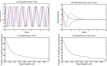
Figure 2: Example eigenfunctions for (a) stationary periodic and (b) non-stationary co-variance functions, both with period 10 units. Also, the number of significant eigenfunctions for input length scales, l, for the (c) stationary periodic and (d) non-stationary covariance function.
To demonstrate the eigenfunction approach to representing Gaussian process priors via a finite basis, Figure 2(a) shows example eigenfunctions for a stationary periodic Mat´ern process. The Mat´ern kernel is defined (Rasmussen and Williams, 2006) as
Mat´ern(τ, ν, σ, l) =σ22 1−ν Γ(ν)
√ 2ν l τ !ν ˇ Kν √ 2ν l τ ! , (31)
where τ ≥ 0, Γ and ˇKν are the gamma and modified Bessel functions, respectively, ν indicates the order, σ is the output scale which governs the amplitude of the kernel and
l is the input length scale which governs the smoothness of the kernel. When the target function is periodic it is a direct function of the periodphase,κ(τ) =|sin(πτ /D)|whereD
is the function period. Consequently, the periodic Mat´ern is given by Mat´ern(κ(τ), ν, σ,l). The periodic Mat´ern is of particular interest to us as it is used in Section 8 to model customer call centre arrival rates and in Section 9 to model the residual dynamics within home heating.
covari-ance function, and consequently the magnitude of the basis function, we would be unable to determine the phase of the basis function. KPCA, in contrast, is able to determine both the magnitude, and consequently phase, of the Fourier basis functions.
A key property of the KPCA approach is that the eigenfunctions are not limited to the Fourier basis and, consequently, KPCA is also able to model non-stationary periodic covariance functions efficiently, in which case the eigenfunctions, which are inferred using KPCA from the non-stationary covariance function, are anharmonic as we will now demon-strate. Figure 2(b) shows the first three most significant eigenfunctions for an exponentially moderated periodic kernel
K(t, t0) = Mat´ern(κ(t−t0), ν, σ, l) exp −|t| − |t0|
. (32)
Figure 2, panels (c) and (d) show how the number of significant eigenfunctions decreases with increasing kernel smoothness for both the harmonic and anharmonic kernels above. The smoothness of the kernel is parameterized by the phase length scale, l. As above, we choose to declare an eigenfunction as significant if its eigenvalue is more than one hundredth of the maximum eigenvalue. Although this is a conservative definition of significance we can see that only a small number of basis functions are required to model these kernels.
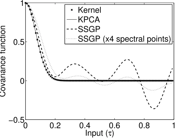
We now compare the SSGPR, described above, and the eigenfunction approaches to modelling stationary kernels. For stationary kernels both the SSGPR and eigenfunction methods use a linear basis model with sinusoidal basis functions. The only difference be-tween the approaches is that SSGPR assigns basis function frequencies (called spectral points) by sampling the kernel power spectrum. Both sine and cosine functions are used for each frequency. The KPCA infers its frequencies deterministically from the kernel and uses the basis functions with the most significant eigenvalues. Each spectral point corre-sponds to a Fourier basis function with known frequency with indeterminate phase. So,
S spectral points produce S Fourier basis functions which has the same complexity as S
Fourier basis functions in the eigenfunction approach. We compare the efficacy of both linear basis approaches when representing the squared-exponential kernel. The SSGPR was specifically developed with this kernel in mind and thus we present the fairest comparison. In order to investigate this difference and isolate the inference procedure by which the GP hyperparameters are learned from the data, the SSGPR algorithm is changed only slightly so that the actual kernel hyperparameters used correspond to the actual hyperparameters of the model which generated the training data. We also use the known generative GP hyperparameters within the eigenfunction model.
SSGPR covariance function approximation differed by as much as 0.23 (that is, 23% of the prior function variance). Clearly, the eigenfunction model is a much more accurate repre-sentation of the actual generative kernel even when using only a quarter of the number of basis functions as the SSGPR.
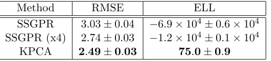
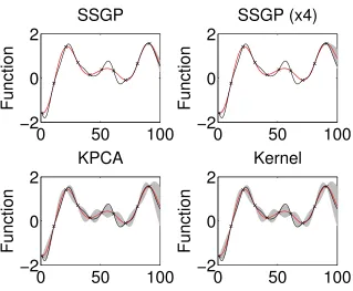
The error in the SSGPR representation of the covariance function can have a signifi-cant impact on the accuracy of GP inference as the SSGPR can signifisignifi-cantly underestimate the posterior variance of the target function. To illustrate the extent of this problem, Figure 4 shows the posterior distributions of a sparsely measured function inferred using Equations (2) and (3) and the SSGPR and eigenfunction approximations of the covariance functions. Clearly, the SSGPR variances in the top two panes are less than those calculated using the squared-exponential model (bottom right pane) and the approximate eigenfunc-tion model (lower left pane). Furthermore, Table 1 compares the RMSE and expected log likelihood for the SSGPR and KPCA approaches over 100 functions drawn from the GP. Each function is measured every 10 units, as above, with no measurement noise. The SSGPR propensity to underestimate the posterior variance is demonstrated by a very low expected log likelihood of −6.9×10⁴ compared to 75 for the KPCA eigenfunction method. Even when the number of spectral points is increased four fold the KPCA approach is still more accurate.
In summary, the eigenfunction model is a more efficient representation than the SSGPR in that it identifies an orthogonal basis and consequently requires fewer basis functions to capture the significant features of the generative kernel. Further, as we saw earlier, the eigenfunction approach generalizes to non-stationary kernels which can be represented efficiently by non-sinusoidal basis functions. Consequently, we advocate the eigenfunction approach over the SSGPR approach for generating the basis for use with LFMs.
Method RMSE ELL
SSGPR 3.03±0.04 −6.9×10⁴±0.6×10⁴ SSGPR (x4) 2.74±0.03 −1.2×10⁴±0.1×10⁴
KPCA 2.49±0.03 75.0±0.9
Table 1: RMSE and expected log likelihood for KPCA and SSGPR with the same number of basis functions and also SSGPR with four fold increase in the number basis functions.
In the next section we extend our eigenfunction approach to quasi-periodic latent force models. This is a key contribution of our paper.
6. Representing Quasi-Periodic Latent Forces with Linear Basis Models
0
0.2
0.4
0.6
0.8
1
−0.5
0
0.5
1
Input (
τ
)
Covariance function
Kernel
KPCA
SSGP
SSGP (x4 spectral points)
Figure 3: A comparison of SSGPR and eigenfunction approaches to modelling GP kernels via basis functions. The plots show the covariance functions corresponding to each of the eigenfunction and SSGPR models.
change between cycles. In the home heating application (described in detail in Section 9), where the residual heat within a home is modelled as a latent force, a phase shift in the residual heat profile may arise from cooking dinner at slightly different times from day to day.
When the latent force process,u(t), is not perfectly periodic but exhibits some regularity from cycle to cycle it is called quasi-periodicand is often modelled as the product of two kernels (Rasmussen and Williams, 2006) thus
Kquasi-periodic(t, t0) =Kquasi(t, t0)Kperiodic(t, t0), (33)
where Kperiodic(t, t0) is a periodic kernel (stationary or non-stationary) and Kquasi(t, t0) is
a non-periodic kernel which reduces the inter-cycle correlations. For example, in Roberts et al. (2013), their quasi-periodic kernel is the product of a squared-exponential kernel and a periodic squared-exponential kernel and takes the form
Kquasi-periodic(t, t0) =σ2exp −
(t−t0)2
l2quasi
!
exp
−
sinDπ(t−t0)
periodic
2
l2periodic
. (34)
We note that Equation (32) is also a quasi-periodic covariance function.
We will now demonstrate thatKquasi-periodic(t, t0) can be modelled within the state-space
0
50
100
−2
0
2
SSGP
Function
0
50
100
−2
0
2
SSGP (x4)
Function
0
50
100
−2
0
2
KPCA
Function
0
50
100
−2
0
2
Kernel
Function
Figure 4: A comparison of SSGPR and eigenfunction approaches to modelling GP kernels via basis functions. The plots show typical example function estimates drawn using both approaches. The KPCA uses 22 basis functions and the SSGPR uses 22 spectral points and 88 spectral points respectively. The grey regions are the first standard deviation confidence regions.
dynamically. Equation (21) can be extended to include time varying process weights, a(t) (O’Hagan, 1978) thus
u(t) =X j
aj(t)φj(t). (35)
Consequently, whenu(t) is generated by a quasi-periodic kernel then
Kquasi-periodic(t, t0) =E[u(t) u(t0)] =
X
ij
φi(t)E[ai(t)aj(t0)]φj(t0).
We assume thatai(t) is drawn from a Gaussian process, so that
ai ∼ GP(0, µφiKquasi), (36)
where µφi is the eigenvalue for the eigenfunction, φi, ofKperiodic as per Equation (23). We
also assume that each weight process is independent. Thus
E[ai(t)aj(t0)] =
(
µφiKquasi(t, t0) ifi=j,
Consequently
Kquasi-periodic(t, t0) =
X
i
φi(t)µφiKquasi(t, t0)φi(t0)
= Kquasi(t, t0)
X
i
φi(t)µφiφi(t0)
= Kquasi(t, t0)Kperiodic(t, t0).
We see that the periodic component of the model, Kperiodic, is represented by the basis
function, φ, in the LBM whereas the non-periodic component, Kquasi, is represented via
the time varying LBM coefficients, a. Note that, whereas for the resonator model, as per Equations (18) and (19), the Fourier basis functions, φ, are stochastic functions of time, in the eigenfunction approach, the coefficients, a, are stochastic functions of time and they reassign weight to fixed basis functions, φ(t).
In order to accommodate variant LBM coefficients in the Kalman filter we assume that each LBM coefficient is drawn from a stationary Gaussian process with covariance function,
Kquasi, as per Equation (36). In which case, we can express the eigenfunction weight
Gaussian process, ar(t), as a stochastic differential equation, as per Equation (6), thus
dAr(t)
dt =FrAr(t) +Wr ωr(t), (37)
where the state vector, Ar(t), comprises the coefficient time series and its derivatives,
Ar(t) = (ar(t) dadtr(t),· · · ,d
pr−1a
r(t)
dtpr−1 )T. Thus, as Ar can be expressed as a stochastic dif-ferential equation then it can be inferred using the Kalman filter as demonstrated in Har-tikainen and S¨arkk¨a (2010). We can weaken the stationarity assumption and thus permit a greater choice for Kquasi by allowing changes in Kquasi’s output scale at discrete time
instances called change points.
We propose three forms for Kquasi which are the Continuous Quasi model (CQM), the Step Quasi model(SQM) and theWiener-step Quasi model(WQM). Although many other quasi-periodic forms are possible these models are chosen as they can each be represented efficiently within the Kalman filter state vector, as we will see in Section 7, whilst capturing the key qualitative properties of the data we wish to model. Specifically, the CQM models smooth, continuous deviations from cyclic behaviour over time, and, consequently, closely resembles the quasi-periodic model in Roberts et al. (2013). Alternatively, the SQM and WQM impose stationarity within a cycle but allow for function variation between cycles. We demonstrate that each can be represented in the Kalman filter via a single variable in the state-vector.
6.1 Continuous Quasi Model (CQM)
This stationary model imposes changes in the cycle continuously over timet. It is equivalent to the Mat´ern kernel with orderν = 1/2 expressed as
KquasiCQM(t, t0) =σr2exp
−|t−t
0|
lr
The input hyperparameter, lr, is positive. As the CQM covariance function, KCQM, is a
first order Mat´ern, as per Equation (9), it can be represented as a Markov process, as per Equation (37). The process model, Fr, and white noise spectral density, qr, for the first order Mat´ern are presented in Equations (10) and (11). Reproducing this model here for completeness, if a is drawn from a GP with the quasi-periodic kernel in Equation (38),
ar∼ GP(0, KquasiCQM), then
dar(t)
dt =Frar(t) +ωr(t),
where, ωr(t) is a white noise process with spectral density qr and
Fr =− 1
lr
, qr=
2σ2r√π lr Γ(0.5)
,
and lr and σr are the input and output scales, respectively, as per Equation (38). We note that, by using the CQM kernel as part of the quasi-periodic latent force covariance function, each LBM coefficient, ar(t), can be represented by a single variable in the Kalman filter state vector. In Section 7 we will demonstrate how this continuous time LTI model can be incorporated into a discrete time LFM model.
6.2 Step Quasi Model (SQM)
This model can be used to decorrelate cycles at change points between cycles. This non-stationary model preserves the variance of the periodic function each side of the change point. However, the function’s correlation across the change point is diminished. For times, t and t0, with t and t0 in the same cycle Kquasi-periodic(t, t0) = Kperiodic(t, t0). When
times t and t0 correspond to different cycles then Kquasi-periodic(t, t0) < Kperiodic(t, t0). If N
consecutive cycles are labelled C = 1,2, . . . , N and C(t) denotes the cycle index for timet
then
KquasiSQM(t, t0) =σ2rexp
−|C(t)−C(t
0)|
lr
. (39)
Again, the kernel input hyperparameter, lr, is positive.
6.3 Wiener-step Quasi Model (WQM)
Again, we assume the presence of change points between cycles. This non-stationary model increases the variance of the function at the change point. If N consecutive cycles are labelledC = 1, . . . , N then
Example covariance functions for the three forms forKquasiare shown in Figure 5. Also,
sample quasi-periodic function draws are shown for each kernel. The functions are drawn from a quasi-periodic squared-exponential kernelKquasi-periodic(t, t0) withKperiodic(t, t0) the
periodic squared-exponentialKSE, as per Equation (16), with periodD= 10 units, various
input scales l (specified within each subfigure) and Kquasi(t, t0) set to either KquasiCQM(t, t0), KquasiSQM(t, t0) or KquasiWQM(t, t0). In the case of SQM and WQM a new cycle begins every 10 time units.
The SQM and WQM kernels can be incorporated into the discrete time Kalman filter by firstly expressing them as continuous time differential equations as per Equation (6). Suppose that eitherar∼ GP(0, KSQM) or ar ∼ GP(0, KWQM) then
dar(t)
dt = 0,
everywhere, except at change points. Thus, in the case of SQM and WQM the corresponding processar(t) can be represented via a first order differential equation as per Equation (37) withAr(t) =ar(t), ∆r = 1,Fr= 0 and Wr = 0. However, at a change point,τ, the SQM and WQM covariance functions jump in value as can be seen in Figure 5 at input distances 20 and 40, for example. The value of the process,ar(τ), immediately after the change point is related to the process, ar(τ−), immediately before the jump thus
ar(τ) =G∗rar(τ−) +χ∗r(τ), (41)
whereG∗r is the process model andχ∗r(τ) is a Gaussian random variable,χ∗r(τ)∼ N(0, Q∗r). In Appendix A we demonstrate that the process model,G∗r, and process noise variance,Q∗r, for the SQM at the change point are
G∗r,SQM= exp
−1
lr
(42)
and
Q∗r,SQM=σr2
1−exp
−2
lr
, (43)
respectively. Similarly, Appendix A also shows that the process model, G∗r, and process noise variance, Q∗r, for the WQM at a change point are
G∗r,WQM= 1 (44)
and
Q∗r,WQM=ξr, (45)
0 20 40 60 80 100 0
0.2 0.4 0.6 0.8 1
input distance, |t−t′|
Covariance function
l=50 l=20 l=10
0 20 40 60 80 100
−5 0 5 10 15
input, t
function
l=50 l=20 l=10
(a) CQM Covariance functions (b) CQM Sample functions
0 20 40 60 80 100
0.7 0.8 0.9 1
input, t
covariance function
l=50 l=20 l=10
0 20 40 60 80 100
−5 0 5 10 15
input, t
function
l=50 l=20 l=10
(c) SQM Covariance functions (d) SQM Sample functions
0 20 40 60 80 100
0 200 400 600
input, t
covariance function
ξ=100 ξ=10 ξ=2
0 20 40 60 80 100
−100 0 100 200 300
input, t
Function
ξ=100 ξ=10 ξ=2
(e) WQM Covariance functions (f) WQM Sample functions
Figure 5: Covariance functions (left column) for CQM, SQM and WQM. Also, sample quasi-periodic functions (right column) for CQM, SQM and WQM quasi kernels and a squared-exponential periodic kernel.
The three forms forKquasiwill be applied to both the call centre customer queue tracking
state vector is augmented with periodic or quasi-periodic latent forces that are approximated using the latent force eigenfunctions.
7. Recursive Estimation with Periodic and Quasi-Periodic Latent Force Models
This section describes a state-space approach to inference with LFMs in some detail. We shall treat the periodic and non-periodic latent forces differently when performing inference with them. Following Hartikainen and S¨arkk¨a (2010, 2011), non-periodic forces will be mod-elled using the power spectrum of their corresponding covariance functions. Alternatively, the periodic latent forces will be modelled using the eigenfunctions of the corresponding periodic covariance function. The key idea in this section is to infer the LFM unknowns via the Kalman filter. The unknowns include the non-periodic forces and their derivatives, as per Equation (12), along with the coefficients of the periodic forces, as per Equation (37). The remainder of this section describes in detail how the KF state is predicted forward in time and how measurements of the system are folded into the state estimate.
We examine periodic and quasi-periodic cases separately as state-space inference with periodic latent forces uses a more compact model. For the periodic case, we assume that the latent forces, u, as per Equation (4), can be separated into two distinct sets, periodic forces, up, and non-periodic forces,unp, so that Lu(t) =Lnpunp(t) +Lpup(t) as described in Section 3. Then, Equation (4) becomes
dz(t)
dt =F z(t) +Lnpunp(t) +Lpup(t).
We model non-periodic latent forces and their derivatives, as per Equation (6), and periodic forces using eigenfunctions as per Equation (29). We define the augmented state vector,za, as per Equation (12), and also the corresponding periodic force coefficients,Lap= [LTp, 0T]T so that the forces up still act on z within za thus
dza(t)
dt =Fa za(t) +Laωa(t) +L
a
pup(t), (46)
whereωaand La are as per Equations (13) and (14).
We now introduce our eigenfunction model for the periodic latent forces into Equa-tion (46). First, we consider periodic latent forces, introduced in SecEqua-tion 5, for which the corresponding LBM coefficients,{a}in Equation (29), are constant over time. Substituting our Nystr¨om approximation basis model for the periodic forces, as per Equation (28), into the dynamic differential model, as per Equation (46), we get
dza(t)
dt =Fa za(t) +Laωa(t) +
R
X
r=1
Jr X
j=1
Lap(·, r) ˜φrj(t)arj, (47)
where R is the number of latent forces, Jr is the number of eigenfunctions for latent force
r,arj are the eigenfunction weights and the vectorLap(·, r) is the rth column of the matrix Lap in Equation (46). The Nystr¨om basis function, ˜φrj, is
˜
φrj(t) =
√
Nr
µrj
whereKr,SrandNr are the covariance function, the quadrature points at which the kernel is sampled for forcer, as per Equation (26), and the cardinality ofSr. Theµrj andvrj are the Gram matrix eigenvalues and eigenvectors, respectively.
The differential equations (47) have the solution
za(t) =Φ(t0, t)za(t0) +qa(t0, t) +
R
X
r=1
Jr X
j=1
arjMrj(t0, t), (49)
where, again, Φ(t0, t) denotes the matrix exponential, Φ(t0, t) = exp(Fa(t−t0)), and qa(t0, t)∼ N(0,Qa(t0, t)) where
Qa(t0, t) =
Z t
t0
Φ(s, t)LaΛaLTaΦ(s, t)Tds,
and Λa, as per Equation (15), is the spectral density of the white noise processes corre-sponding to the non-periodic latent forces. The matrixMrj(t0, t) is the convolution of the
state transition model,Φ, with each of the periodic latent force eigenfunctions expressed as
Mrj(t0, t) = √
Nr
µrj
Z t
t0
ds Φ(s, t)Lap(·, r)Kr(s, Sr)
vrj.
For small time intervals [t0, t], which is the case for our applications in Sections 8 and 9, Mrj can be calculated using numerical matrix exponential integration methods. Further, we note Φ(t0,t) is stationary and this can mitigate the need to recalculate this matrix exponential at each instance of the time series.
To accommodate the latent forces within the Kalman filter we must ensure that our discrete time dynamic model, as per Equation (49), has the appropriate form. Specifically
X(t) =G(t0, t)X(t0) +ω(t0, t),
where the noise process, ω, is i.i.d Gaussian and zero-mean. In order to rewrite Equa-tion (49) into the appropriate form for Kalman filter inference we define a vector,a, as per Equation (21), which collects together the eigenfunction weights thus
a= (a11, . . . , a1J1, a21, . . . , a2J2. . .)
T,
and, similarly, a matrix, M, which collects together the convolutions,Mrj, thus
M(t0, t) = (M11(t0, t), . . . ,M1J1(t0, t),M21(t0, t), . . . ,M2J2(t0, t). . .).
We further augment the state vector to accommodate the model weights,a, corresponding to the periodic latent forces. Let
X(t) = (zTa(t),aT)T, (50)
eigenfunction weights, a, required by the periodic forces as per our approach. When the eigenfunction weights are constant we can rewrite Equation (49) thus
X(t) =G(t0, t)X(t0) +ω(t0, t), (51)
where
G(t0, t) =
Φ(t0, t) M(t0, t)
0 I,
(52)
and
ω(t0, t) =
qa(t0, t) 0
.
Thus, predictions of the Gaussian process, X, can be inferred using the Kalman filter. Of course, the model in Equation (51) can also be incorporated within the Kalman Smoother to perform full (that is, forward and backward) regression overX(t) for all timetif required (Hartikainen and S¨arkk¨a, 2010). The prediction equations for the state mean, ¯X(t | t0),
and covariance, P(t | t0), at time t conditioned on measurements obtained up to time t0,
are
¯
X(t|t0) = G(t0, t) ¯X(t0 |t0), (53) P(t|t0) = G(t0, t)P(t0|t0)G(t0, t)T +Q(t0, t), (54)
whereQ(t0, t),
Qa(t0, t) 0
0 0
.
We assume that measurements, y, are Gaussian distributed thus
y(t) =H X(t) +η(t), (55)
whereη is zero-mean multivariate Gaussian,η∼ N(0,Z), whereZis the observation noise covariance matrix and themeasurement model,H, extracts the appropriate elements of the state vector. These measurements can be folded into the Kalman filter in the usual way. The update equations given measurement, y(t), as per equation (55), are
¯
X(t|t) = X¯(t|t0) +K(y(t)−HX¯(t|t0)), (56)
P(t|t) = (I−KH)P(t|t0), (57)
whereK is the Kalman gain given by
K=P(t|t0)HT(HP(t|t0)HT +Z)−1. (58)
Kalman gain will be cubic in the number of measured physical processes. So, although the state vector may be augmented in order to model both physical processes and latent forces, as described above, these additions will not impact on the cost of the matrix inversion in Equation (58).
We next extend our state-space approach to accommodate quasi-periodic latent forces. For the quasi-periodic latent forces the corresponding kernel LBM coefficients, a, are func-tions of time, as per Equation (35). We assume that each LBM coefficient is drawn from a Gaussian process with covariance function, Kquasi, as per Equation (33), and we now
demonstrate how these dynamic weight processes, a(t), are incorporated into the Kalman filter, Equations (53) to (57).
As above, arj, corresponds to the jth eigenfunction for latent force r. However, for quasi-periodic latent forces each eigenfunction weight is variant and we assume arj(t) can be written as a stochastic differential equation, as proposed in Section 6, thus
dArj(t)
dt =FrjArj(t) +Wrj ωrj(t), (59)
where the state vector,Arj(t), comprises derivatives of the coefficient time series,Arj(t) = (arj(t),dadtrj(t),· · · ,d
prj−1
arj(t)
dtprj−1 )
T. We can recover the eigenfunction coefficient from A rj thus
arj(t) =∆rjArj(t),
where the vector∆rj = (1,0, . . . ,0) is an indicator vector which extracts the LBM coefficient
arj fromArj. Thus, the latent force,ur(t), as per Equation (35), is
ur(t) =X j
arj(t)φrj(t) =
X
j
φrj(t)∆rjArj(t), (60)
whereφrj is thejth eigenfunction for the latent forcer. Substituting our Nystr¨om approx-imation for the eigenfunction,φ(t) as per Equation (28), into Equation (60) we get
ur(t) =
X
j
√
Nr
µrj
[Kr(t, Sr)]vrj∆rjArj(t).
Then, substitutingur into the differential latent force model, Equation (47), we get
dza(t)
dt =Fa za(t) +Laωa(t) +
R
X
r=1
Jr X
j=1
mrj(t)Arj(t), (61)
where R is the number of latent forces, Jr is the number of eigenfunctions for latent force
r,La and ωa(t) are as per Equations (13) and (14) and the vectormrj is
mrj(t) =
√
Nr
µrj
Lap(·, r)Kr(t, Sr)
vrj∆rj, (62)
the Gram matrix eigenvalues and eigenvectors, respectively. The vector Lap(·, r) is the rth column of the matrixLap in Equation (46).
Now, as for the constant eigenfunction coefficient case, to exploit the Kalman filter for LFM inference with quasi-periodic latent forces we gather together all the LFM Gaussian variables, za and {Arj}, into a single state-vector. In so doing, we define a vector A(t) which collects together the eigenfunction coefficients and their derivatives thus
A(t),(A11(t)T,A12(t)T, . . . ,A21(t)T,A22(t)T, . . . ,)T, (63)
a matrix m(t) which collects together the vectors{mrj}thus
m(t),(m11(t),m12(t), . . . ,m21(t),m22(t), . . . ,),
a matrixFAwhich collects together the process models for all eigenfunction coefficients for
all latent forces, as per Equation (59) thus
FA,blockdiag(F11,F12. . . ,F21,F22, . . .),
a vectorωAwhich collects together the noise processes for the non-periodic forces,ωa, as per Equation (61), and noise processes for all the eigenfunction coefficients as per Equation (59) thus
ωA,(ωaT, ω11, ω12, . . . , ω21, ω22, . . .)T, (64)
and the block diagonal matrix LA which collects together the corresponding process noise
coefficients,La, as per Equation (61) and Wrj as per Equation (59) thus
LA ,blockdiag(La,W11,W12. . . ,W21,W22, . . .).
As per Equation (50) let
X(t),(zTa(t),AT(t))T, (65)
be our augmented state vector which now accommodates the derivative auxiliary variables required by the non-periodic forces as per Hartikainen and S¨arkk¨a (2011) and the eigen-function weights required by the quasi-periodic forces as per our approach. Combining Equations (59) and (61) we get
dX(t)
dt =
Fa m(t)
0 FA
X(t) +LAωA(t), (66)
where ωA(t) is a vector of independent white noise processes. The spectral density of the
ith white noise process in this vector is [ΛA]i where
ΛA= (Λa, q11, q12, . . . , q21,, q22, . . .).