Some Extensions of Positive and Negative Rules for Discovering Basic Interesting Rules

(1)

Published online August 30, 2013 (http://www.sciencepublishinggroup.com/j/ijiis) doi: 10.11648/j.ijiis.20130204.12

Some extensions of positive and negative rules for

discovering basic interesting rules

Nguyen Duc Thuan

Dept. Information Systems of Nha Trang University, Khanh Hoa, Vietnam

Email address:

[email protected]

To cite this article:

Nguyen Duc Thuan. Some Extensions of Positive and Negative Rules for Discovering Basic Interesting Rules. International Journal of Intelligent Information Systems.Vol. 2, No. 4, 2013, pp. 64-69. doi: 10.11648/j.ijiis.20130204.12

Abstract:

Positive reasoning and negative reasoning have been applied to be very useful in practice as clear from the record of many real life applications, especially in medicine. These reasoning mechanisms play important role in cutting the search space, reflecting experts' decision, supporting decision by the cooperation of experts and computers. This paper proposes the concepts of extended negative rule, minimal rule and explores their properties. Furthermore, an algorithm for finding all minimal positive rule and minimal negative rule is given. This algorithm is effective to discover positive and negative rules which have not redundant formula. These rules support to deduce the other important positive and negative rules. Experiments are carried out on data sets of UCI machine learning repository to analyze the performance study.

Keywords:

Positive Rule, Negative Rule, Minimal Rule, Minimal Positive Rule, Minimal Negative Rule

1. Introduction

Traditional classification rules take the deterministic or probabilistic form as if X then Y (X→Y). The common feature of both deterministic and probabilistic rules is that they reduce their consequence positively if an example satisfies their conditional parts. The reasoning by these rules can be called positive reasoning. But this form as rules couldn’t improve classification accuracy sharply because it is not easy to improve the matured algorithms.

In many applications, the most typical is in medicine, experts use not only positive reasoning but also negative reasoning of selection of candidates, which is represented as if –then rules whose consequences include negative term. New rules in form of X→Y, X→Y, X→Y are introduced into data mining.

In recent years negative rule mining got much focus. Many of the algorithms developed for mining positive and negative rule. The concept of negative relationships mentioned for the first time in the literature by Brin et.al (1997). To verify the independence between two variables, they use the statistical test. To verify the positive or negative relationship, a correlation metric was used. Their model is chi-squared based. The chi-squared test rests on the normal approximation to the binomial distribution (more precisely, to the hyper geometric distribution). This approximation breaks

down when the expected values are small. Wu et al (2004) discussed how to use negative association rule and designed constraint to reduce the search space. Ji and Tan (2004) studied how to inducing negative and positive rules for gene expression, which also based on association rules. Tsumoto (2001) use positive and negative rules which based on rough sets to predict clinical case. This paper presents some results concerning extended positive and negative rules, which proposed by Tsumoto [7]. The main result is effective to discover positive and negative rules which have not redundant formula. These rules support to deduce the other important positive and negative rules. Moreover, this paper also proposes the concepts of extended negative rule for discovering interesting potential negative rules.

The structure of this paper is as follows:

Section 2 recalls some basic concepts: information system, formula, classification accuracy and coverage, positive and negative rules. Section 3 presents our results and experiments on UCI data sets. We summarize our research and discuss some future work directions in the section 4.

2. Basic Concepts

(2)

2.1. Information System

Let U denote a nonempty finite set called the universe and A denote a nonempty, finite set of attributes, i.e., a: U→Va, ∀a∈A, where Va is called the domain of a,

respectively. Then a decision table is defined as an information system S=(U,A∪{d}).

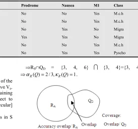
For example, Table 1 is an information system with U={1,2,3,4,5,6} and A={Age, Location, Nature, Prodrome, Nausea, M1} and d = Class. For Location ∈ A, VLocation is

defined as {Occular, Whole, Lateral}.

Table 1. An example of a data set

No Age Location Nature Prodrome Nausea M1 Class

1 2 3 4 5 6

50 – 59 40 – 49 40 – 49 40 – 49 40 – 49 50 – 59

Occular Whole Lateral Whole Whole Whole

Persistent Persistent Throbbing Throbbing Radiating Persistent

No No No Yes No No

No No Yes Yes No Yes

Yes Yes No No Yes Yes

M.c.h M.c.h Migra Migra M.c.h Pyscho

2.2. Formula

Atomic formulas over B⊆A∪{d} are expression V of the form [a=v], called descriptors over B, where a∈B and v∈Va.

The set F(B, V) of formulas over B is the least set containing all atomic formulas over B and closed with respect to disjunction, and negation. For example, [location=occular] is a descriptor of B.

For each f ∈ F(B, V), fS is the set of all objects in S

satisfy f, defined inductively as follows: 1.If f = [a = v] then fS = {s ∈ U | a(s) = v}.

2. (f

∧

g)S = fS

∩

gS; (f

∨

g)S = fS

∪

gS;

(

¬

f)S = U – fS

Example 1: In the preceding example, with Table 1 f = [Location = Whole] ⇒ fS = {2, 4, 5, 6}

g = [Location = Whole]

∧

[Nausea = No]

⇒_g_S_{= {2, 4, 5, 6}}

∩

{1, 2, 5} = {2, 5}.

2.3. Classification Accuracy and Coverage

2.3.1. Definition 1

Let R and Q denote a formula in F(B,V), R is a formula over the conditional attribute set A, Q is a formula over the decision attribute set D={d}. Classification accuracy and coverage (true positive rate) for R→Q is is defined as:

A D A R

R Q R

Q)= ∩

(

α (1)

D D A R

Q Q R

Q)= ∩

(

κ (2)

where |S|,αR(Q),κR(Q),denote the cardinaliry of a set S, a classification accuracy of R as to classification of Q, and coverage (a true positive rate of R to Q) respectively.

Example 2: As show in Table 1, R = [Nausea=Yes] ⇒ RS = {3, 4, 6}

D = [Class = Migra]⇒ QD= {3, 4}

⇒RS∩QD = {3, 4, 6}

∩

{3, 4}={3, 4} ⇒α_R(Q)=2/3,κ_R(Q)=1.

Figure 1. Venn diagram of accuracy and coverage

2.4. Atomic Rule

RuleR→Q is a atomic rule if R is a atomic formula.

2.5. Positive Rule

RuleR→Q is a positive rule if

]

[ _j _k

j a v

R=∧ = and α_R(Q)=1.0.

Thus, RuleR→Q is a positive rule ⇔RS ⊆QD

Example 3: As show in Table 1, R= [Age=50-59]∧[Location=Whole]

⇒_R_S_={1, _6}_∩_{2, _4, _5, _6}={6} _and

Q=[Class=Psycho]⇒DS={6} ⇒

α

R

(

Q

)

=

1 /

1 =

1 .

0

.

Thus,[Age=50-59]∧[Location=Whole] → [Class=Psycho] is a positive rule.

Rule R→Q is an atomic positive rule if R is atomic formula and R→Q is a positive rule.

Example 4: As show in Table 1,

(3)

Thus, [Nausea=No] → Q=[Class=M.c.h] is an atomic positive rule.

2.6. Exclusive Rule and Negative Rule

2.6.1. Definition 5 (Exclusive Rule)

Rule R→Q is an exclusive rule if

]

[ _j _k

j a v

R=∨ = and κ_R(Q)=1.0

Thus, if rule R→Q is a exclusive rule then DS⊆RS⇒

Q→R is a positive rule. We also have Q→R ⇔¬R→¬Q.

2.6.2. Definition 6 (Negative Rule)

Rule R→Q is a negative rule if R=∧_j¬[a_j =v_k], ]

[d vd

Q=¬ = and ∀[aj =vk],κ[aj=vk]([d=vd])=1.0. If j=1 then negative rule is an atomic negative rule. Example 5: As show in Table 1, we have

[Nature=Persistent]∨[Location=Whole]→[Class=M.c.h] is an exclusive rule.

¬[M1=Yes]∧¬[Nausea=no]→ ¬[Class=M.C.h] is a negative rule.

Figure 2 Venn diag. for positive rule.

Figure 3. Venn diag. for neg. rule.

3. Main Results

3.1. Extended Negative Rule

From definition 6, the discovery of the negative rules is very difficult, because having to check all atomic formulas involved these rules:

(∀[aj =vk],κ[aj=vk](D)=1.0), here D=[d=vd]

This condition also missed some sense as a negative rule in practice. Thus, we propose definition extended negative rule follow:

3.1.1. Definition 7 (Extended Negative Rule)

Rule R→Q be a extended negative rule if ]

[ _j _k

j a v

R=∧ ¬ = , Q=¬[d =v_d] and

0 . 1 ]) ([

' = d =

R d v

κ . Here R’=∨_j[a_j =v_k].

Obviously, negative rule is a special case of the extended negative rule. The difference between negative rule and extended negative rule can be seen Venn diagram:

Figure 4. Venn diagram for negative rule

Figure 5. Venn diagram for extended negative rule

∀i=1,2,3, Ri→Q is not a negative rule, but R→Q is a

extended negative rule.

Example 6: As show in Table 1, we have Q= ¬[Class=M.c.h], R1= f=[Nature=Persistent],

R2= g = [Location=Whole].

Let Q’= Q ⇒

Q

_D'

=

{

1 ,

2 ,

5 }

, f_S ={1,2,6} , } 6 , 5 , 4 , 2 { = S g 0 . 1 3 2 ) ' ( 1 ' ' ≠ = ∩ = D D S Q Q f Q R κ ; 0 . 1 3 2 ) ( ' ' '

2 = ≠

∩ = D D S R Q Q g Q κ 0 . 1 3 3 ) ( ) ( ' ' ' ' = = ∩ ∪ = D D S S R Q Q g f Q κ Therefore,

R→Q⇔¬[Naure=Persistent]∧¬[Location=Whole]→¬[Cla ss=M.c.h] is not negative rule, but it is extended negative rule.

3.2. Minimal Rule

(4)

If R→Q is both a positive (negative/extende negative/ exclusive) rule and a minimal rule then R→Q is called minimal (negative/extende negative/ exclusive) rule.

Example 7: As show in Table 1 We have:

a.[Age = 50 – 59]

∧

[Location = Whole] → [Class = Psycho] is positive rule.

If remove [Age = 50 – 59] then [Location = Whole] →

[Class= Psycho]is not a positive rule.

If remove [Location = Whole] then [Age = 50 – 59] →

[Class= Psycho] is not a positive rule.

Therefore, [Age = 50 – 59]

∧

[Location = Whole] →

[Class = Psycho] is a minimal positive rule. b.Let R = [M1 = Yes]

∨

[Location = Whole]

⇒ RS = {1, 2, 5, 6}

∨

{2, 4, 5, 6} = {1, 2, 4, 5, 6},

with D = [Class = M.c.h] ⇒ DS = {1, 2, 5} ⊆ RS ⇒ R → D is an exclusive rule

⇒ (¬[M1 = Yes]

∧

¬[Location = Whole]) →¬[Class

= M.c.h] is an extended negative rule.

But, we have: ¬[M1 = Yes] → ¬[Class = M.c.h] is an extended negative rule.

Therefore, (¬[M1 = Yes]

∧

¬[Location = Whole]) → ¬[Class = M.c.h] is not minimal extended negative rule.

We have some properties of minimal rule:

3.2.2. Proposition 1

If[a=v]→[d=u] is an atomic positive rule then [a=v] is not appear in any minimal positive rule that the left hand side there is more than one formula.

If [a=v]→[d=u] is an atomic positive rule then any formula:

R=

∧

_j

[

a

_j

=

v

_k

]

we have [a=v]∧R→[d=u] is an positive rule.

If ¬[a=v]→ ¬[d=u] is an atomic negative rule then [a=v] ] is not appear in any minimal negative rule that the left hand side there is more than one formula.

Proposition 1, proposition 2 and proposition 3 are obtained from definitions 1, 3, 6, 8.

If f =[a=v],D=[d=u] and f_S ∩D_S =0 then any R∈F(B,V), we have:

a.

f

∧

R

→

D

is not positive rule.

b. Let

R

'

=

f

∨

R

then

¬

R

'

→

¬

D

is not minimal negative rule.

Proof

a. Fromf_S ∩D_S =0, it is obviously that f ∧R→D

is not positive rule.

b. Suppose ¬R'→¬Dis a minimal negative rule

⇒ DS⊆ R’S, we have and f_S∩D_S =0 ⇒ DS ⊆ RS ⇒_¬R→¬D is a negative rule, a contradiction (because

D

R →¬

¬ ' _{is a minimal negative rule}_{). The proof is}

complete.

3.2.5. Algorithm for Finding all Minimal Positive and Minimal Negative Rules

Tsumoto (2005) gave an algorithm for deduce all positive and negative rules based on rough set theory. Xindong Wu, ChengQi Zhang and Shichao Zhang (2005), Alatas và Akin (2006), presented algorithms mining of both positive and negative associate rules. Tinghuai Ma, Jiazhao Leng, Mengmeng Cui and Wei Tan (2009) proposed RGCA algorithm to deduce negative and positive rules. The RGCA algorithm based on rough set, records are processed item-by-item. In RGCA algorithm, for the rule reduction that based on classification attribute, it does not need to deal with records one by one so that to improve calculation efficiently.

In this paper, the main result is effective to discover positive and negative rules which have not redundant formula. From proposition 1, 2, 3, 4, we proposed an algorithm for finding all minimal positive and negative rules as follow:

Input: S=(U,A∪{d}); L = {[aj=vk] | aj∈A, vk∈Vaj}; D =

[d= di]

Output: RPos, RNeg: set of minimal positive rule and set of minimal negative rule respectively

Method

La = L

For each di ∈Dom(d) do

{//induct atomic positive and negative rules and

candidate set can generate minimal positive and negative rules}

Lp = La; Ln = La

For each R = [aj = vk] in La do

{ Caculate αR(D) and κR(D);

If αR(D) = 1.0 then

{ Pos = Pos ∪ {R}; La = La – {R};

Lp = Lp – {R};

Ln = Ln – {R}; }

If κR(D) = 1.0 then

{ Neg = Neg ∪ {R}; Ln = Ln – {R}; }

If αR(D) = κR(D) = 0 then

{ Lp = Lp – {R};

Ln = Ln – {R}; }

}

For i = 2 to n do // n =|A|

{LPi = { j i

j

R

∧

=1

|

R

_j

∈

L

_p

,

R

_k

≠

R

_m

,

when k≠ m}

LNi= { j i

j

R

∨

=1

|

R

_j

∈

L

_p

,

R

_k

≠

R

_m

,

when k≠ m}}

For each R = ∧i[aj = vk] in LPi do

{ if αR(D) = 1.0 then

{ Pos = Pos ∪ {R}; LPi = LPi – {R};}

if αR(D) = 0 then LPi = LPi – {R};}

For each R = ∨i[aj = vk] in LNi do

if κR(D) = 1.0 then

(5)

// Generate minimal positive and negative rules

LPos = {R→[d=di]| R∈Pos};

LNeg={¬R→¬[d=di]|R∈Neg};}

The worst-case complexity of inducing minimal positive and minimal negative rules is:

O( | ( )| | ( )|

| |

1

d dom a

dom

A

i i

×

∑

= )

3.3. Experiment Results

We use data sets from UCI repository of machine learning databases and domain theories to verify the extended negative rule concept and the presented algorithm above.

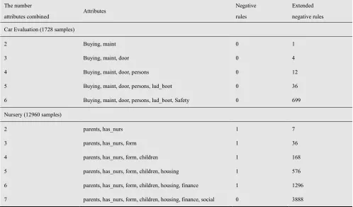
Table 2 summarizes our analysis results, which shows the number of negative rules and extended negative rules.

For Car Evaluation dataset, if we consider only two attributes Buying and Maint then the number of negative rule (definition 6) is zero, but there is one extended negative rule (definition 7):

¬[Buying=low] ^ ¬[Maint=low] → ¬[Class=good]. Similarly, if we consider three attributes Buying, Maint, Door, the number of negative rule (definition 6) is zero, but there are four extended negative rules (definition 7):

1. ¬[Buying=low] ^ ¬[Maint=low] ^ ¬[Doors=2] → ¬[Class=good]

4. ¬[Buying=low] ^ ¬[Maint=low] ^ ¬[Doors=5more] → ¬[Class=good]

We can see that the expansion of the negative rules to avoid omitting the rule mean in practice.

4. Conclusion and Future work

Our study is mainly focused on mathematical properties of negative rules and minimal rules. In this paper we introduced the concept of extended negative rules, which extracts hidden knowledgeable useful information from medical databases. Furthermore, an algorithm to generate all minimal positive and minimal negative rules is introduced.

Interestingly, very few have focused on negative association rules due to the difficulty in discovering these rules. Although some researchers pointed out the importance of negative associations, only few groups of researchers proposed an algorithm to mine these types of associations. This not only illustrates the novelty of negative association rules, but also the challenge in discovering them.

Experiment results with some data sets from UCI repository of machine learning databases showed the meaning of these extensions of positive and negative rules.

In future we wish to conduct experiments on some other real datasets and compare the performance of our algorithm with other related algorithms.

Table 2. Comparision between the number of negative rules and the number of extended negative rules

The number attributes combined

Attributes Negative

rules

Extended negative rules Car Evaluation (1728 samples)

2 Buying, maint 0 1

3 Buying, maint, door 0 4

4 Buying, maint, door, persons 0 12

5 Buying, maint, door, persons, lud_boot 0 36

6 Buying, maint, door, persons, lud_boot, Safety 0 699

Nursery (12960 samples)

2 parents, has_nurs 1 7

3 parents, has_nurs, form 1 36

4 parents, has_nurs, form, children 1 168

5 parents, has_nurs, form, children, housing 1 576

6 parents, has_nurs, form, children, housing, finance 1 1296

(6)

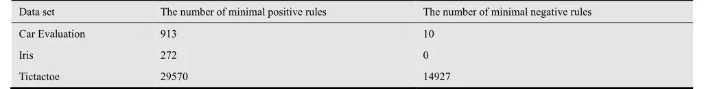
Table 3. Comparision between the number of negative rules and the number of extended negative rules

Data set The number of minimal positive rules The number of minimal negative rules

Car Evaluation 913 10

Iris 272 0

Tictactoe 29570 14927

References

[1] B.Kavitha Rani, K.Srinivas, B.Ramasubba Reddy, Dr.A.Govardhan, “Mining Negative Association Rules”, International Journal Of Engineering and Technology, Vol.3 (2), 100-105, 2011

[2] Brin S, Motwani R, Silverstein cristiano Beyond market: Generalizing association rules to correlations [A]. Processing of the ACM SIGMOD Conferrence 1997 [m]. New York: ACM Press,265-276, 1997

[3] Chris Cornelis, Peng Yan, Xing Zhang, Guoqing Chen, Mining Positive and Negative Association Rules from Large Databases, IEEE Conference Cybernetics and Intelligent Systems, BangKok, June 2006

[4] D.R. Thiruvady and G.I.Webb, Mining Negative Rules using GRD, Advances in Knowledge Discovery and Data Mining, Lecture Notes on Computer Science Vol 3056, pp 161-165. Proceedings of the 8th Pacific-Asia Conference, PAKDD (2004) Sydney, Australia, May 26-28, 2004

[5] E.Ramaraj, N.Venkatesan, “Positive and Negative

Association Rule Analysis in Health care Databases”, IJCSNS International Journal of Computer Science and Network Security, Vol 8 (10), October, 2008

[6] Maria-Luiza, Antonie Osmar R. Za¨ıane, Mining Positive and Negative Association Rules:An Approach for Confined Rules, 8th European Conference on Principles and Practice of Knowledge Discovery in Databases, Pisa, Italy, September 20-24, 2004

[7] Nikhil R.Pal, Lakhmi Jain (Eds), Advanced Techniques in Knowledge Discovery and Data Mining, Springer-Verlag London Limited , 233-252, 2005

[8] Tinghuai Ma, Jiazhao Leng, Mengmeng Cui and Wei Tian, “Inducing Positive and Negative Rules Based on Rough Set”, Infomation Technology Journal 8(7): 1039-1043, 2009 [9] Xingdong Wu, ChengQi Zhang, Shichao Zhang, “Efficient

Mining of Both Positive and Negative Association Rules”, ACM Transactions on Information Systems, Vol. 22, No. 3, July, 2004