Published online September 20, 2014 (http://www.sciencepublishinggroup.com/j/jeee) doi: 10.11648/j.jeee.20140203.11
ISSN: 2329-1613 (Print); ISSN: 2329-1605 (Online)
An efficient fractional-pixel motion compensation based on
Cubic convolution interpolation
Lung-Jen Wang
*, Chia-Tzu Shu
Dept. of Computer Science and Information Engineering, National Pingtung University, Pingtung, Taiwan, R. O. C.
Email address:
[email protected] (Lung-Jen Wang)
To cite this article:
Lung-Jen Wang, Chia-Tzu Shu. An Efficient Fractional-Pixel Motion Compensation Based on Cubic Convolution Interpolation. Journal of Electrical and Electronic Engineering. Vol. 2, No. 3, 2014, pp. 47-54. doi: 10.11648/j.jeee.20140203.11
Abstract:
The fractional-pixel motion compensation is used in the H.264/AVC algorithm, in order to improve the coding efficiency of fractional-pixel displacement, an efficient cubic convolution interpolation (CCI) with four coefficients is proposed. In this paper, the detailed derivation of the CCI filter and using CCI with fractional-pixel displacement are presented. It is shown by computer simulation that the presented method substantially reduces the computation complexity and also increases the precision of the motion compensation.Keywords:
H.264/AVC, Motion Compensation, Fractional-Pixel Displacement, Cubic Convolution Interpolation1. Introduction
A video can be viewed as a time-ordered sequence of images-frames [1]. In general, the volume of uncompressed video data is so large that the use of video compression is almost mandatory. In High Definition TV (HDTV), if uncompressed, the bitrate could easily exceed 1Gbps. Therefore, video compression allows the video to be transmitted over the Internet in real time. Also it reduces the requirements for video storage.
The H.264/AVC algorithm is one of the latest international standard for the video compression technique, which was jointly implemented by ITU-T video coding experts group (VCEG) and ISO/IEC motion picture experts group (MPEG) [2][3]. In order to improve the precision for motion compensation prediction in the H.264/ AVC algorithm [4]-[8], the fractional-pixel displacement is calculated, which is used the interpolation process to estimate the fractional-pixel (1/2- and 1/4-) positions between the existing positions. In the H.264/ AVC standard, there are two processing steps in the fractional-pixel displacement. First, a fixed 6-tap Wiener filter is calculated for the 1/2-pixel displacement, and then the bilinear interpolation is used for the 1/4-pixel displacement. The disadvantage of the H.264/ AVC standard is that the computations required for 1/2-pixel displacement with 6-tap Wiener filter are substantially increased. The 6-tap Wiener filter requires not only huge computational cost, but also its accuracy is not guaranteed in the fractional-pixel
displacement [7].
Interpolation is the process of estimating the intermediate values of a continuous event from discrete samples. It is used extensively in image processing to magnify or reduce images and to correct spatial distortions. Because of the amount of image data, an efficient interpolation algorithm is essential. Rigorously speaking, the process of decreasing the data rate is called decimation and increasing the data samples is termed interpolation [9]-[11][16]-[18]. It is well known that several decimation and interpolation functions such as linear interpolation [10], cubic convolution interpolation [11], cubic B-spline interpolation [16], linear spline interpolation [17], cubic spline interpolation [9][18], etc. can be used in the image processing.
This paper is organized as follows. Section 2 describes the background of this work for the interpolation function, H.264/AVC algorithm and interpolation in fractional-pixel displacement. Then the proposed CCI filter with four coefficients (4-tap CCI) is presented in Section 3. In this section, the cubic convolution function and 4-tap CCI are discussed in detail. In Section 4, the proposed CCI combined with motion compensation is illustrated for the H.264/AVC algorithm. The motion compensation with CCI and the CCI interpolation computation are also described in detail. Finally, experimental results and conclusions are discussed in Sections 5 and 6, respectively.
2. Background of this Work
2.1. Interpolation Functions
An interpolation function is a special type of approximating function. A fundamental property of interpolation functions is that they must coincide with the sampled data at the interpolation nodes, or sample points. In other words, if f is a sampled function, and if fˆ is the
corresponding interpolation function, then fˆ(xk)= f(xk) whenever xk is an interpolation node [11]. Thus, an interpolation function can be expressed in the following form.
∑
=
− = N
k
k k kR x x
c x f
1
) ( )
(
ˆ
(1)
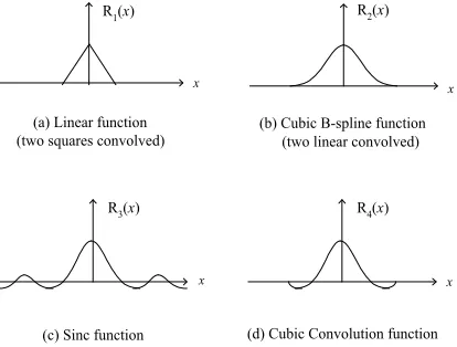
where ck = f(xk) are the coefficients to be determined from the input data, Rk(x) is the chosen interpolation basis function, x and xk represent continuous and discrete value, respectively, and N is the number of given data points. There are several interpolation functions, shown in Fig. 1, such as linear function, cubic B-spline function, sinc function, and cubic convolution function [10][11].
(a) Linear function (two squares convolved)
R1(x)
x
(b) Cubic B-spline function (two linear convolved)
R2(x)
x
(d) Cubic Convolution function R4(x)
x
(c) Sinc function R3(x)
x
Figure 1. Several interpolation functions.
The linear function provides the first-order linear sample interpolation with triangle-shaped interpolation waveforms. This linear function may be considered to be the result of convolving a square function with itself. It requires only one addition and one shift in each interpolation. The convolution of the linear function with itself yields a cubic B-spline function. The cubic B-spline function is a particularly attractive candidate for image interpolation because of its properties of continuity and smoothness at the sample points [10]. The sinc convolution function uses many sample points for each interpolation point. It provides an exact reconstruction, but it cannot be physically generated by an incoherent optical filtering system [10]. It is possible to approximate the sinc function by truncating its tails. That is to say if we only consider the sinc function with a four sample interval. The problem is that the slope discontinuity at the ends of the sinc waveform will lead to amplitude ripples in a reconstructed function. In order to eliminate amplitude ripples in a reconstructed function, the cubic convolution interpolation is developed to force the slope of the ends of interpolation to be zero [11].
2.2. The H.264/AVC Algorithm
The H.264/AVC standard is the latest algorithm of video compression technique [2][3]. The block diagram of the H.264/AVC encoder is shown in Fig. 2. In this figure, the input video frame is partitioned into some blocks. For each block of input video frame, the H.264/AVC encoder applies either intra-frame prediction or inter-frame prediction to process the video signal. In the intra-frame prediction, each block is converted by the DCT transform into the DCT coefficients. Next the quantization (Q) and the entropy coding (ENC) are used for the DCT coefficients. In the inter-frame prediction, which is also called as the motion compensated prediction or temporal prediction, the motion estimation uses the current frame block from reference frames to predict the content of the current frame block [15]. Furthermore, the de-quantization (Q-1) and the inverse DCT (IDCT) transform are used to obtain the reconstructed video frame.
2.3. Interpolation in Fractional-Pixel Displacement
In the H.264/AVC algorithm, the displacement vectors with fractional-pixel resolution are applied to perform the motion compensated prediction. In order to estimate and compensate the fractional-pixel displacement, the two-step interpolation process is used in [7]. In H.264/AVC, the block diagram of the two-step interpolation process is shown in Fig. 3. In the first step, the sampling rate of image I is increased by a factor of 2 and filtered by the 6-tap Wiener filter with the six coefficients: [1, -5, 20, 20, -5, 1]/32 is used to interpolate the 1/2-pixel positions in this step and an image Iw is generated
two coefficients: [1, 1]/2 is used to interpolate the 1/4-pixel positions and an image I′ is generated after the second step.
In Fig. 4, the interpolation relationship between the full-pixel positions (black), the 1/2-pixel positions (gray) and the 1/4-pixel positions (white) are shown. In this figure, at first, the 1/2-pixel positions aa, bb, b, q, cc, dd, and ee, ff, h, l, gg, hh are calculated, using a horizontal or vertical 6-tap Wiener filter, respectively. For example, aa = (A1 - 5A2 + 20A3 + 20A4 - 5A5 + A6) / 32, and ee = (A1 – 5B1 + 20C1 + 20D1 – 5E1 + F1) / 32, respectively. Using the same Wiener filter applied at 1/2-pixel positions aa, bb, b, q, cc, and dd, the 1/2-pixel position j is obtained as: j = (aa – 5bb + 20b + 20q – 5cc + dd) / 32. In the second step, the remaining 1/4-pixel positions are computed using the bilinear interpolation filter based on the calculated 1/2-pixel positions and existing full-pixel positions [8]. For example, a = (C3 + b) / 2 and d = (C3 + h) / 2 in horizontal and vertical interpolations, respectively.
Figure 2. Block diagram of the H.264/AVC encoder.
W I
Figure 3. Two-step interpolation process used in H.264/AVC.
A1 A2 A3 A4 A5 A6
B1 B2 B4 B5 B6
C1 C2 C4 C5 C6
D1 D2 D4 D5 D6
E1 E2 E4 E5 E6
F1 F2 F4 F5 F6
aa B3 C3 D3 E3 F3 bb cc dd
ee ff gg hh
b
a c
d e f g h i j k m n o p
l
q
Figure 4. Interpolation relationship.
3. Cubic Convolution Interpolation
3.1. The Cubic Convolution Function
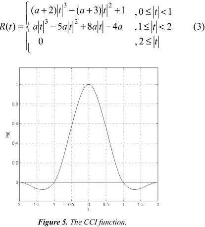
The cubic convolution function was given in [11], which is composed of piecewise cubic polynomials defined on the subintervals (-2, -1), (-1, 0), (0, 1), and (1, 2). Outside the interval (-2, 2), the function is zero. The function kernel must be symmetric. As a consequence of this condition, the cubic convolution function is defined by
+ + + + + + = 0 )
( 2 3 2 2 2 2
1 1 2 1 3 1 D t C t B t A D t C t B t A t R 2 , 2 1 , 1 0 , t t t ≤ < ≤ < ≤
(2)
where R(0)=1 , R(±1)=R(±2)=0 and R(t) and R′(t) are continuous at
t
= 0, 1, 2 and R′(±2)=0 . In (2),2 2 2 1 1 1
1 ,B ,C ,D ,A ,B ,C
A and D2 are eight unknown
coefficients. To solve these coefficients, Keys in [11] supposes A2 =a , then the remaining seven unknown coefficients can be determined in terms of
a
. That is, the cubic-convolution function in (2) can be expressed in terms of a as − + − + + − + = 0 4 8 5 1 ) 3 ( ) 2 ( )
( 3 2
2 3 a t a t a t a t a t a t R 2 , 2 1 , 1 0 , t t t ≤ < ≤ < ≤ (3)
Figure 5. The CCI function.
Furthermore, Keys in [11] also uses A2 = a = -1/2, finally,
the cubic convolution function, shown in Fig. 5, is given by
( )
(
)
(
)
(
)
3 2
3 2
3/2 5 2 1, 0 t 1
1 2 5 2 4 2, 1 t 2
0, 2 t
t / t
R( t ) / t / t t
− + ≤ <
= − + − + ≤ <
≤
(4)
3.2. 4-Tap Cubic Convolution Interpolation
Let τ be a fixed, positive integer. Also, let X(t) be the full-pixel samples in the current frame, where 0≤t≤n−1, and X0,⋯,Xn−1 be the n existing full-pixel samples in
the reference frame. The shift function of the cubic convolution function can be defined as Rk(t)=R(t−kτ) for 0≤k≤n−1. Then the fractional-pixel displacement
) ( ˆ t
X in the reference frame by the cubic convolution interpolation (CCI) as
∑
∑
− = − = − = = 1 0 1 0 ) ( ) ( ) ( ˆ n k k n k kkR t X R t k
X t
X τ (5)
where R(t) is the cubic convolution function in (4). The
fractional-pixel function Xˆ(t) in (5) is the CCI function of
the full-pixel samples X0,⋯,Xn−1 in the reference frame.
One can be find the function Xˆ(t) in (5) that minimize the
prediction error of Xˆ(t) to X(t) is defined by
∑
− = − = 1 0 ) ( ˆ ) ( ) ( n t t X t X te (6)
Thus, the sequence of n fractional-pixel values Xˆ(t) in (5) can be obtained by the CCI function and used for the 1/2-pixel and 1/4-pixel displacements, respectively, in the H.264/AVC motion compensation. Furthermore, the fractional-pixel displacement Xˆ(ta) between the two adjacent existing full-pixel samples Xk and Xk+1 in the reference frame is illustrated in Fig. 6 and given by the sum of the CCI function,
1 2 2 1 1 1 1 for ) ( ) ( ) ( ) ( = ) ( ˆ + + + + + − − < < + + + k a k a k k a k k a k k a k k a t t t t R X t R X t R X t R X t X (7) k
t
tk+1 tk+31 − k t 2 − k t 3 − k
t tk+4
a t k X 1 − k
X Xk+1
2 + k X 1 − k R k R 1 + k R 2 + k R 2 + k t ) ( ˆ t X ) ( ˆ a t X t ∆ a t ∆
Figure 6. The fractional-pixel interpolation between samples.
In (7) and Fig. 6, let ∆t=tk+1−tk and ∆ta =ta−tk, then the displacement from ta to tk−1,tk+1andtk+2 are
t t t
ta− k−1=∆a+∆ , ta−tk+1=∆ta−∆t , and ta−tk+2 = t
ta− ∆
∆ 2 , respectively.
Table 1. List of CCI coefficients for fractional-pixel displacement
fractional-pixel displacement CCI coefficients
1/2-pixel displacement [-1, 9, 9, -1]/16
1/4-pixel displacement [-9, 111, 29, -3]/128
3/4-pixel displacement [-3, 29, 111, -9]/128
In order to calculate the fractional-pixel displacement, if we set ∆t=1 and ∆ta=1/2 , then the 1/2-pixel displacement can be given by
(
1 9 9 1 2)
16 1 = ) (
ˆ − − + + + − +
k k k k
a X X X X
t
X (8)
Moreover, if we set ∆t=1and ∆ta =1/4 , then the 1/4-pixel displacement can be given by
(
9 1 111 29 1 3 2)
128 1 = ) (
ˆ − − + + + − +
k k k k
a X X X X
t
X (9)
That is, if we set ∆t=1and ∆ta =3/4, then the 3/4-pixel
displacement can be given by
(
3 1 29 111 1 9 2)
128 1 = ) (
ˆ − − + + + − +
k k k k
a X X X X
t
X (10)
In (8)-(10), the CCI filter with four coefficients (4-tap CCI) for the fractional-pixel (1/2-, 1/4- and 3/4-) displacements are summarized in Table 1.
4. Using CCI in Motion Compensation
4.1. Motion Compensation with CCI
W
I
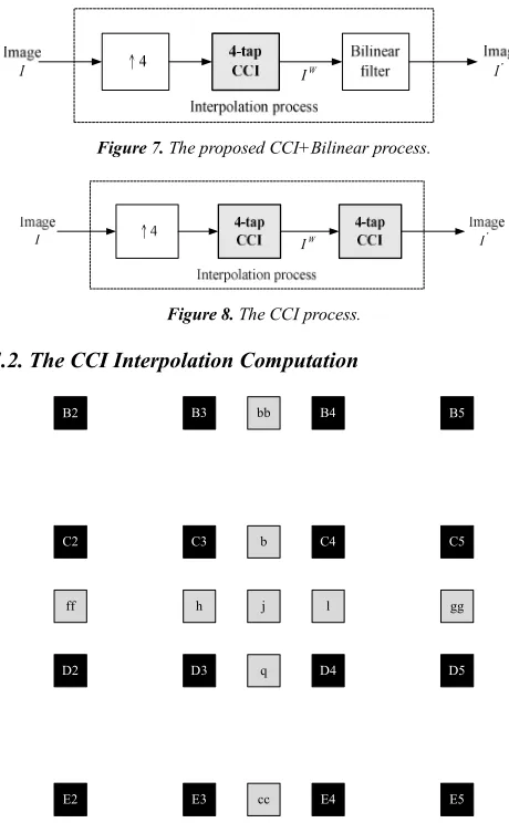
Figure 7. The proposed CCI+Bilinear process.
W
I
Figure 8. The CCI process.
4.2. The CCI Interpolation Computation
B2 B4 B5
C2 C4 C5
D2 D4 D5
E2 E4 E5
B3
C3
D3
E3
bb
cc
ff gg
b
h j l
q
Figure 9. 1/2-pixel CCI operations: full-pixel positions (black); 1/2-pixel positions (gray).
In Fig. 9, the 4-tap CCI interpolation is used to interpolate the 1/2-pixel positions and the 1/2-pixel CCI operations are illustrated: full-pixel positions (black); 1/2-pixel positions (gray). For example, b = (-C2 + 9C3 + 9C4 - C5) / 16. In Figs. 10 and 11, the 4-tap CCI interpolation is also applied to interpolate the 1/4-pixel and 3/4-pixel positions in horizontal and vertical interpolations, respectively. Fig. 10 shows the 1/4-pixel and 3/4-pixel CCI operations in horizontal interpolations: full-pixel (black); 1/2-pixel (gray); 1/4-pixel (white); 3/4-pixel (blue). For example, a = (-9C2 + 111C3 + 29C4 – 3C5) / 128, and c = (-3C2 + 29C3 + 111C4 – 9C5) / 128, respectively. In addition, Fig. 11 shows the 1/4-pixel and 3/4-pixel CCI operations in vertical interpolations: full-pixel (black); 1/2-pixel (gray); 1/4-pixel (white); 3/4-pixel (blue). For example, d = (-9B3 + 111C3 + 29D3 – 3E3) / 128, and m = (-3B3 + 29C3 + 111D3 – 9E3) / 128, respectively.
5. Experimental Results
The proposed CCI+Bilinear and CCI methods, which are described in Section 4 and shown in Figs. 7 and 8, respectively, are implemented in Microsoft visual C++ program and compared with the H.264/AVC standard method (labeled as
Standard), which Wiener filter and bilinear filter are used for the fractional-pixel displacement. These three algorithms are based on the JM 18.0 [13]. For the simulation common conditions of the H.264/AVC algorithm, the most important settings are summarized in Table 2.
The objective performance is measured by the peak signal to noise ratio (PSNR) and given by
2
10
255 10
Y
Y PSNR log ( dB ),
MSE
=
(11)
where MSEY is the mean-square error between the original Y
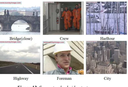
image and reconstructed Y image for the YUV format. Some standard QCIF (Bridge(close), Crew, HarBour, Highway), CIF (Bridge(close), Bridge(far), Foreman) and 4CIF (City, Crew, HarBour) frame sequences are selected and shown in Fig. 12. Performance comparisons are carried out on the above these frame sequences. All the experimental results (bit rates and PSNR performance) are computed from the reconstructed Y images.
B2 B4 B5
E2 E4 E5
B3
E3
bb
cc
C2 C4 C5
D2 D4 D5
C3
D3
ff gg
b
a c
h j l
q
i k
Figure 10. 1/4-pixel and 3/4-pixel CCI operations in horizontal
interpolation: full-pixel (black); 1/2-pixel (gray); 1/4-pixel (white); 3/4-pixel (blue).
B2 B4 B5
E2 E4 E5
B3
E3
bb
cc
C2 C4 C5
D2 D4 D5
C3
D3
ff gg
b
a c
d e f g
h i j k
m n o p
l
q
Figure 12. Some standard video test sequences.
Table 2. Most important H.264/AVC coder settings [14]
Parameter Settings
Profile: High
Number of reference images: 4
Number of B coded frames: 2
Sequence type: I-B-B-P-B-B-P
Hierarchical Coding: off
Weighted prediction: on
Rate-distortion optimization: on
Search range: 32 for QCIF and CIF
64 for 720p and 1080p
YUV format 4:2:0
Quantization parameter (I/P/B): 22/23/24, 27/28/29, 32/33/34, 37/38/39
For the computational complexity of the fractional-pixel displacement in the Standard (H.264/AVC), CCI+Bilinear and CCI methods, the number of addition(+), multiplication(*), and shift(>>) are estimated and compared in Table 3 and Table 4. Obviously, in Table 3, the estimated operation number of the proposed CCI+Bilinear method is less than those of both Standard and CCI methods. That is, the proposed CCI with bilinear (CCI+Bilinear) method is more fast and efficient than those of the H.264/AVC standard (Standard) and the CCI methods. In other words, for the number of operations, CCI+Bilinear < Standard < CCI.
In Table 4, in terms of the number of addition(+), multiplication(*) and shift(>>) operations, the CCI+Bilinear method is less than the H.264/AVC standard (Standard)
method by 152064, 76032 and 76032 for QCIF sequence, by 608256, 304128 and 304128 for CIF sequence, and by 2433024, 1216512 and 1216512 for 4CIF sequence, respectively. Thus, the proposed CCI+Bilinear method achieves a superior performance in the fractional-pixel displacement than the H.264/AVC standard method.
Table 3. Number of operations for three methods.
Methods Operations QCIF CIF 4CIF
Standard + 684288 2737152 10948608
(H.264/AVC) * 228096 912384 3649536
>> 684288 2737152 10948608
CCI+Bilinear + 532224 2128896 8515584
* 152064 608256 2433024
>> 608256 2433024 9732096
CCI + 1140480 4561920 18247680
* 1368576 5474304 21897216
>> 2433024 9732096 38928384
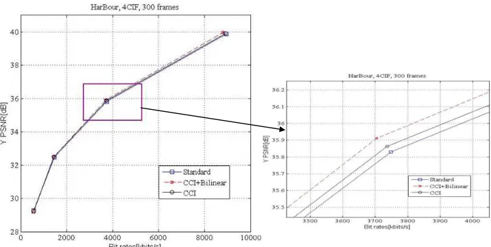
Some experimental results of the rate-distortion curves for the Standard (H.264/AVC), CCI+Binear and CCI methods are compared and shown in Figs. 13, 14 and 15. As shown in these three figures, the proposed CCI+Bilinear and CCI methods obtain the better PSNR values of reconstructed Y image than the Standard (H.264/AVC) method. That is, for the same bit rates, the PSNR values of the Y images, obtained by the CCI+Bilinear and CCI methods are higher than the Standard (H.264/AVC) method by 0.05 dB and 0.02 dB for QCIF sequence, by 0.04 dB and 0.02 dB for CIF sequence, and by 0.14 dB and 0.06 dB for 4CIF sequence, respectively.
Table 4. Comparison of operations for Standard and CCI+Bilinear.
Methods Operations QCIF CIF 4CIF
Standard + 684288 2737152 10948608
(H.264/AVC) * 228096 912384 3649536
>> 684288 2737152 10948608
CCI+Bilinear + 532224 2128896 8515584
* 152064 608256 2433024
>> 608256 2433024 9732096
“Standard” + 152064 608256 2433024
minus * 76032 304128 1216512
“CCI+Bilinear” >> 76032 304128 1216512
Figure 14. Rate-distortion comparison for CIF sequence Bridge(close).
Figure 15. Rate-distortion comparison for 4CIF sequence HarBour.
6. Conclusions
The H.264/AVC algorithm is the international standard for video compression. In the H.264/AVC standard, the fractional-pixel displacement is used in the motion compensated prediction. There are two processing steps in the fractional-pixel motion compensation. In the first step, a fixed 6-tap Wiener filter is used for the 1/2-pixel displacement. The second step is to use the bilinear interpolation for the 1/4-pixel displacement. In this paper, the 4-tap CCI filter is proposed to reduce the computational complexity of the 1/4-pixel displacement and also increase accurately the motion compensated prediction. In addition, the derivation of CCI filter and CCI combined with motion compensation are discussed in detail. Finally, some computer simulations show that the proposed CCI algorithm with the bilinear interpolation can be used to speed up the H.264/AVC standard and also obtains a superior performance for motion compensation.
Acknowledgements
This work was supported by the National Science Council,
R.O.C., under Grant NSC 102-2221-E-251-005.
References
[1] Z. N. Li and M. S. Drew, Fundamentals of Multimedia. Pearson Prentice Hall, 2004.
[2] T. Wiegand, G. J. Sullivan, G. Bjontegaard, and A. Luthra, “Overview of the H.264/AVC video coding standard,” IEEE Trans. on Circuits and Systems for Video Technology, vol. 13, no. 7, pp. 560-576, July 2003.
[3] T. Wiegand and G. J. Sullivan, “The H.264/AVC video coding standard [Standards in a Nutshell],” IEEE Signal Processing Magazine, vol.24, no.2, pp.148-153, March 2007.
[4] T. Wedi, “Adaptive interpolation filter for motion compensated hybrid video coding,” in Proc. Picture Coding Symposium (PCS), Seoul, Korea, Jan. 2001.
[6] T. Wedi and H. G. Musmann, “Motion- and aliasing-compensated prediction for hybrid video coding,” IEEE Trans. on Circuits and Systems for Video Technology, vol. 3, no. 7, pp. 577-587, Jul. 2003.
[7] T. Wedi, “Adaptive interpolation filters and high-resolution displacements for video coding,” IEEE Trans. on Circuits and Systems for Video Technology, vol. 16, no. 4, pp. 484-491, Apr. 2006.
[8] Y. Vatis and J. Ostermann, “Adaptive interpolation filter for H.264/AVC,” IEEE Trans. on Circuits and Systems for Video Technology, vol. 19, no. 2, pp. 179-192, Feb. 2009.
[9] T. K. Truong, L. J. Wang, I. S. Reed, and W. S. Hsieh, “Image data compressing using cubic convolution spline interpolation,” IEEE Trans. on Image Processing, vol.9, no.11, pp.1988-1995, Nov. 2000.
[10] W. K. Pratt, Digital Image Processing, second edition. John Wiley & Sons, Inc., New York, 1991.
[11] R. G. Keys, “Cubic convolution interpolation for digital image processing,” IEEE Trans. on Acoustic, Speech, and Signal Processing, vol. 29, no.6, pp.1153-1160, Dec. 1981.
[12] L. J. Wang and C. T. Shu, “A fast efficient fractional-pixel displacement for H.264/AVC motion compensation,” in Proc.
of the 28th IEEE International Conference on Advanced Information Networking and Applications (AINA-2014), pp.25-30, Victoria, Canada, May 13-16, 2014.
[13] H.264/AVC Reference Software Version JM18.0, available online at: http://iphome.hhi.de/suehring/tml/download/old_jm/
[14] T. K. Tan, G. Sullivan, and T. Wedi, Recommended simulation common conditions for coding efficiency experiments, ITU-T Q.6/SC16, Doc. VCEG-AE10, Jan. 2007.
[15] Y. Ye, G. Motta, and M. Karczewicz, “Enhanced adaptive interpolation filters for video coding,” in Proc. Data Compression Conference (DCC), pp. 435-444, March 2010.
[16] M. Unser, A. Aldroubi, and M. Eden, “B-spline signal processing: Part II-Efficient design and applications,” IEEE Trans. Signal Processing, vol. 41, pp. 834-848, Feb. 1993.
[17] I. S. Reed and A. Yu, Optimal Spline Interpolation for Image Compression, United States Patent, No. 5822456, Oct. 13, 1998.