Modeling and Prediction of Changes in Anzali Pond Using Multiple Linear Regression and Neural Network

(1)

Published online November 11, 2014 (http://www.sciencepublishinggroup.com/j/ijiis) doi: 10.11648/j.ijiis.s.2014030601.29

ISSN: 2328-7675 (Print); ISSN: 2328-7683 (Online)

Modeling and prediction of changes in Anzali Pond using

multiple linear regression and neural network

Farshad Parhizkar Miandehi

*

, Erfan Zidehsaraei, Mousa Doostdar

Department of Computer Engineering, Zanjan Branch, Islamic Azad University, Zanjan, Iran

Email address:

[email protected] (F. P. Miandehi), [email protected] (E. Zidehsaraei), [email protected] (M. Doostdar)

To cite this article:

Farshad Parhizkar Miandehi, Erfan Zidehsaraei, Mousa Doostdar. Modeling and Prediction of Changes in Anzali Pond Using Multiple Linear Regression and Neural Network. International Journal of Intelligent Information Systems. Special Issue: Research and Practices in Information Systems and Technologies in Developing Countries. Vol. 3, No. 6-1, 2014, pp. 103-108. doi: 10.11648/j.ijiis.s.2014030601.29

Abstract:

Iranian ponds and water ecosystems are valuable assets which play decisive roles in economic, social, security and political affairs. Within the past few years, many Iranian water ecosystems such asUrmia Lake, Karoun River and Anzali Pond have been under disappearance threat. Ponds are habitats which cannot be replaced and this makes it necessary to investigate their changes in order to save these valuable ecosystems. The present research aims to investigate and evaluate the trend of variations in Anzali Pond using meteorological data between 1991-2010 by means of GMDH, which is based upon genetic algorithm and is a powerful technique in modeling complex dynamic non-linear systems, and linear regression technique. Input variables of both methodsinclude all factors (inside system and outside system factors) which affect variations in Anzali Pond. Exactness of linear regression method was 78% and exactness of GMDH neural network method was more than 97%. As as result, exactness of GMDH neural network method is significantly better than regression model.

Keywords:

Anzali Pond, Regression Analysis, GMDH Neural Network

1. Introduction

Investigation of conditions of natural ecosystems like jungles, range, lakes and ponds is of great importance in every country [3]. At present, Iran uses its natural resources 3.6% more than its normal use.Iranian environment will be disappeared if this trend continues[2]. Within the past few years, many Iranian natural ecosystems like Urmia Lake, Arasbaran jungles and Anzali Pond have received irreparable harms and are prone to complete disappearance [1]. Ponds are important natural ecosystems which cannot be replaced and they cannot be revived if they are not safeguarded. This makes it necessary to investigate the trend of their changes [4]. One of the uninvestigated points about ponds is absence of attention to non-linear changes and behavioral nature of them, which can be affected by many factors [10]. Therefore, the present research tries to model the trend of ponds changes using linear regression and GMDH neural network methods and compare their prediction exactness. It is necessary to understand and model relationship between input-output data in order to model any system. Fuzzy logic, neural networks and genetic algorithm are good techniques in solving complex non-linear systems [9-15-16]. Numerous studies have been

(2)

we analyzed the trend of changes in area and depth of Anzali Pond using linear regression. In the next step, we predicted a time series for changes in Anzali pond using GMDH neural network based on genetic algorithm and used all factors affecting changes in the pond. 70% of data were used as input and 30% were used as test. Results showed that exactness of prediction of area and depth in regression analysis was 78% and in GMDH neural network method was 98%. General structure of this paper is as follows:

In the second part, we review definitions and methods. In the third section, factors influencing on changes in Anzali Pond are introduced. In the fourth section, the influence of the factors on the trend of pond changes is investigated and in the fifth section, we will investigate the implementation and evaluation of the trend of changes using linear regression and GMDH neural network method. In the sixth section, we present conclusions and recommendations.

2. Definitions and Methods

2.1. Multiple Linear Regression

These models are the most widely used of all regression methods. There are two or more predictor variables that may be measurement or qualitative (dummy) variables. Some multiple regression models may contain one measurement variable in multiple forms.

More often, the response variable is influenced by more than one predictor variable. For example, its diameter, height, species, age, and soil fertility may affect timber volume or crown surface of a tree. The crop yield may be affected by amount of irrigation as well as fertilizer.

Unlike simple linear regression, where the response is a straight line, the response may be a curvilinear or multi-dimensional, represented by a hyper-plane or a more complex surface.

Multiple implies more than one predictor variable and linear means linear in the regression coefficients being additive. Examples of two variable linear models are

Y =β0 + β1X1 + β2X2 + ε (1)

a first order linear model with two predictor variables; First order model implies that there is no interaction and the effects of changes in predictor variables are additive. And

Y =β0 + β1X + β2X2 + ε (2)

polynomial regression model with one variable with higher power.

Y =β0 + β1X + β2(1/X) + ε (3)

with transformed predictor variable (1/X).

log(Y) = β0 + β1X1 + β2X2 + ε (4)

with X2 qualitative response variable;

Y =β0 + β1X1 + β2X2 + ε (5)

where X2 is a qualitative indicator variable such as gender

(male, female). Indicator variables that take on the values of 0 or 1 are used to identify the class of a qualitative variable.

2.2. GMDH Neural Network

The GMDH algorithm uses estimates of the output variable obtained fromsimple primeval regression equations that include small subsets of input variables. To elaborate on the essence of the approach, we adhere to the following notation. Let the original data set consist of a column of the observed values of the output variable y and N columns of the values of the independent system variables, that is x = x1; x2; . . , . The primeval equations form a PD which comes in the form of a quadratic regression polynomial

= + + + + +

In the above expression A; B; C;D; E; and F are parameters of the model, u; v, are pairs of variables standing in x whereas z is the best fit of the dependent variable y.

The generation of each layer is completed within three basic steps [5-6-7]:

Step 1. In this step we determine estimates of y using primeval equations.

Here, u and v are taken out of all independent system variables x1, x2,.., . In this way, the total number of polynomials we can construct via (1) is equal to . The resulting columns of values, m = 1,2,…,N(N-1)/2.contain estimates of y resulting from each polynomial that are interpreted asnew ‘‘enhanced’’ variables that may exhibit a higher predictive power than the original variables being just the input variables of the system, x1, x2, . . . , .

Step 2. The aim of this step is to identify the best of these new variables andeliminate those that are the weakest ones. There are several specific selectioncriteria to do this selection. All of them are based on some performance index (mean square, absolute or relative error) that express how the values ( )follow the experimental output y. Quite often the selection criterion includes an auxiliary correction component that ‘‘punishes’’ a network for its excessive complexity. In some versions of the selection method, we retain the columns ( ) for which the performance index criterion is lower than a certain predefined threshold value. In some other versions of the selection procedure, a prescribed number of the best is retained. Summarizing, this step returns a list of the input variables. In some versions of the method, columns of x1, x2; . . . ,. are replaced by the retained columns of z1, z2, . . . , zk , where k is the total number of the retained columns. In other versions, the best k retained columns are added to columns x1; x2; . . . , to form a new set of the input variables. Then the total number N of input variables changes to reflect the addition of values or the replacement of old columns with new total number of input variables.

(3)

immediately by repeating step 1 as described above, otherwise we proceed with step 3.

Step 3 consists of testing whether the set of equations of the model can befurther improved [14]. The lowest value of the selection criterion obtained duringthis iteration is compared with the smallest value obtained at the previous one.

If an improvement is achieved, one goes back and repeats

steps 1 and 2,otherwise the iterations terminate and a realization of the network has beencompleted. If we were to make the necessary algebraic substitutions, we would have arrived at a very complicated polynomial of the form which is also known as the Ivahnenko polynomial

= + ∑ + ∑ ∑ + ∑ ∑ ∑ + ⋯ (6)

where a, , , and so forth are the coefficients of the polynomial.

2.3. Criteria for Prediction Power Measurement

Different criteria have been introduced for measuring prediction power of different models. The followings are several of these criteria:

Root square mean error (RSME):

RMSE=!∑'()_{$ '(}"# _$^+ _$& (7)

Mean absolute error (MAE):

MAE=∑'()_{$ '(}* _$^+ _$*/ℎ (8) Mean absolute prediction error (MAPE):

MAPE=∑ -./^_.(./

/0

-'()

$ '( /ℎ (9)

3. Factors Affecting the Trend of Changes

in Anzali Pond

Thepresent research aims to model and predict the trend of changes in area and depth of Anzali pond. Table 1 shows factors affecting changes in area of the pond and table 2 shows factors affecting changes in the depth of the pond.

Table 1. Independent and dependent variables for modeling and prediction of changes in area of the pond [3].

variables constants Intended atmospheric parameters

X1 B1 Precipitation-independent

X2 B2 Water discharged in river-independent

X4 B4 Temperature-independent

Y Pond surface area-dependent

Table 2. dependent and independent variables for modeling and prediction of depth of water in the pond [3].

variables constants Intended atmospheric parameters

X1 B1 Precipitation-independent

X2 B2 Water discharged in river-independent

X3 B3 Temperature-independent

X4 B4 Debris-independent

Y Pond depth-dependent

4. Investigation of Factors Affecting the

Trend of Changes in Lake

4.1. Using Multiple Linear Regression

In regression analysis, the depth and surface area of the pond were considered as dependent variables and atmospheric parameters were considered as independent variables and the regression equation is as follows:

Y=B0+B1X1+B2X2+B3X3+B4x4+…

Xs are atmospheric parameters and Bs are calculated in a way that least squares index is satisfied.

On the other hand, comparison of B coefficients reveals the rank and impact size of each of the factors.

4.1.1. Depth Investigation

As it was mentioned in section 3, atmospheric data are independent variables in linear regression and elevation of pond level is as presented in table 2. We reach the following equation after investigation of data and variables. the calculated determination coefficient is equal to 0.72.

Y=124.36+0.0551X1+0.00291X2-0.3658X3

4.1.2. Surface Area Investigation

Investigation of the data and variables leads us to the following equation and coefficients. The corresponding determination coefficient is equal to 0.83.

Y=1265.1202.3X1+0.987X2-217.0074X3 (10) tities and variables, but not Greek symbols. Use a long dash

Figure 1. trend of changes in precipitation level in 1991-2010. y = 10.902x - 20552

R2_{= 0.5088}

0 200 400 600 800 1000 1200 1400 1600

1990 1995 2000 2005 2010 2015

(4)

Table 3. data needed for GMDH neural network.

Year Volume of discharged debris (tons)

Volume of discharged water

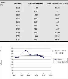
(million cubic meters) rain(mm) evaporation(MM) Pond surface area (Km 2₎

1991 974.44 1600 1095 1100 57.84

1993 990.759 1700 1246 950 58

1998 1073.616 3100 1154 1020 81.87

2001 1175.728 1900 1324 900 66.9

2005 1273.572 1800 1257 850 66.5

2006 1273.189 1700 1425 800 66

2007 1273.158 2000 1326 900 64.5

2008 1272.214 1900 1411 800 62.09

2009 1271.144 1800 1324 1000 60.39

2010 1291.52 1700 1264 900 56.91

Figure 2. trend of changes in the volume of water discharged in Anzali Pond in 1991-2010.

Figure 3. trend of temperature changes in 1991-2010.

Figure 4. level of debris inserted into Anzali Pond in 1991-2010.

Figure 5. changes in the pond's surface area in 1991-2010.

4.2. Modeling and Prediction of Changes in Anzali Pond Using GMDH Neural Network

Primary assumptions in GMDH neural network analysis are as follows:

The number of latent layers is equal to 3.

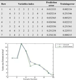
Percentage of the samples considered for test is equal to 30%. in the first layer yields 6 answers and combination of these 6 answers in the second layer yields 21 answers and in the third layer, we obtain 231 layers. For the case of 4 variables for pond depth calculation, we obtain 1540 answers. However, it is necessary to select the best answers out of all answers in order to avoid neural network's divergence. Therefore, training error and prediction error was calculated for all final combinations. Selection of optimal answers seeks two targets: minimization of modeling error and prediction. Another point in selection of optimal final input is observation of the order of selected variables to avoid scattering. As it can be seen in figures (4) and (5), 10 samples were selected for estimation of surface area of the pond and 7 samples were selected for estimation of pond depth using genetic algorithm. Rows 5 and 8 were considered for calculation of the trend of changes due to maintaining the order of input variables.

y = -6.7055x + 15350 R2_{= 0.011}

0 500 1000 1500 2000 2500 3000 3500

1990 1995 2000 2005 2010 2015

Series1 Linear (Series1)

y = -9.1254x + 19198 R2_{= 0.4053}

0 200 400 600 800 1000 1200

1990 1995 2000 2005 2010 2015

y = 36.978x + 983.56 R2_{= 0.7818}

0 200 400 600 800 1000 1200 1400 1600

1991 1993 1998 2001 2005 2006 2007 2008 2009 2010

y = -0.0701x + 204.58 R2_{= 0.0042}

0 10 20 30 40 50 60 70 80 90

1990 1995 2000 2005 2010 2015

(5)

Table 4. table of selection of variables for surface area.

Row Variables index Prediction

error Trainingerror

1 3 3 2 1 2 1 1 2 0.015425 0.000159

2 3 1 3 2 2 1 1 2 0.025124 0.000541

3 3 2 2 1 1 2 2 2 0.065321 0.002124

4 3 3 3 3 3 1 2 3 0.025413 0.251256

5 3 1 2 1 3 3 2 2 0.025125 0.002514

6 3 2 2 1 1 1 2 2 0.365214 0.000215

7 2 2 2 3 3 2 3 3 0.895636 0.005112

8 1 3 1 2 1 1 2 3 0.021212 0.000113

9 2 2 2 3 3 3 1 1 0.521545 0.008955

10 2 1 1 2 2 1 3 3 0.854123 0.005455

Table 5. table of selection of variables for depth.

Row Variables index Prediction

error Trainingerror

1 4 1 2 3 2 1 1 4 0.013333 0.002154

2 4 3 3 2 1 2 4 1 0.025214 0.251546

3 4 2 1 1 3 4 3 2 0.032565 0.003251

4 1 2 3 3 3 4 3 2 0.026566 0.022212

5 3 2 4 1 1 2 3 4 0.025556 0.251561

6 4 4 3 2 2 1 1 1 0.251254 0.225511

7 3 4 2 1 1 2 3 4 0.254136 0.000215

Inputs were classified in two categories: training data (including at least 70% of data) and test data (30% of data). tables 6 and 7 indicate the exactness of depth and surface area evaluation.

Estimations of the coefficients of this model were presented in the previous sections. Prediction of the estimated model by means of linear regression in the time period using equations (7) and (8) reveals that error percentage of the linear regression model for prediction of trend of depth changes is 9.3% and also RMSE for surface area was 7.3%. real data and predicted data using both methods can be observed in figures (8) and (9).

Figure 8. real data graph and linear regression line equation figure for pond surface area.

Figure 9. real data figure and GMDH neural network for pond surface area.

5. Discussion and Conclusion

(6)

References

[1] Tavakkoli, B and SabetRaftar, K. investigation of the impact of area, population and population compression factors of water basin on rivers discharging Anzali Pond, journal of environmental studies: special notes on Anzali pond: 51 to 57, 2007.

[2] Zebardast, L, Jafari, H. R, evaluation of the trend of changes in Anzali Pond using remote sensing and presentation of a managerial solution, journal of environmental studies, 57-64, 2011.

[3] Jamalzad, F, determination of the level of sensitivity of different areas of Anzali Pond using GIS, master degree thesis, environment faculty, Tehran University, page 52, 2008.

[4] Ghahraman, A and Attar, F. Anzali Pond in death coma (an ecological-floristic investigation). Journal of environmental studies: special notes on Anzali Pond: 1 to 38.

[5] Abrishami, Hamid and Moeeni, Ali and Mehrara, Mohsen and AHrari, Mahdi and SoleimaniKia, Fatemeh (2008), "modeling and prediction of gasoline price using GMDH neural network", quarterly of Iranian economic studies, 12th year, number 36, pp: 37-58.

[6] Sharzei, Gholam Ali and AHrari, Mahdi and Fakhraee, Hasan (2008), "structural models, time series and GMDH neural network", journal of economic studies, number 84, pp: 151-175.

[7] Abrishami, Hamid and Mehrara, Mohsen and Ahrari, Mahdi and Mir Ghasemi, Soudeh (2009), "modeling and prediction of Iranian economic growth with a GMDH neural network approach", journal of economic studies, number 88, pp: 1-24.

[8] Ozesmi, S. L., E. M., Bauer. “Satellite Remote Sensing of Wetlands. Wetlands Ecology and, Management”, Vol.10, pp.381-402, 2002.

[9] Abbaspour, M. and Nazaridoust, “Determination of Environmental Water Requirements of Lake Urmia, Iran: an Ecological Approach”, International Journal of Environmental Studies, Vol.64, pp.161-169, 2007.

[10] Zhaoning, G., et al. “Using RS and GIS to Monitoring Beijing Wetland Resources Evolution”, IEEE International, Vol.23, pp.4596 – 4599, 2007.

[11] De Roeck, E., Jones, K., “Integrating Remote Sensing and Wetland Ecology: a Case Study on South African Wetlands”, pp.1-5, 2008.

[12] Yung, J.L., “Sustainable Wetland Management Strategies under Uncertainties”, the Environmentalist, Vol.19, pp. 67-79, 2008.

[13] van Stappen, G., Bossier, P., Sepehri, H., Lotfi, V., RazaviRouhani, S., Sorgeloos, P., “Effects of Salinity on Survival,Growth, Reproductive and Life Span Characteristics of Artemia Populations from Urmia Lake and Neighboring Lagoons”, Journal of Biological Sciences, Vol.11, pp.164-172, 2008.

[14] Howland. J.C, Voss. M.S. “Natural Gas Prediction Using the Group Method of Data Handling”, ASC. . (2003)

[15] Ivakhnenko.G.A (1995),”The Review of Problems Solvable by Algorithms of the Method of Data Handling (GMDH)”, Pattern Recognition and Image Analysis, Vol.5, No.4, PP 527-535.

[16] Ivakhnenko. G.A and Muller. J.A. (1996). “Recent Development of Self-Organizing Modeling in Prediction and Analysis of Stock Market”, Available in URL Address: http://www.inf.kiev.ua/GMDH Home/Articles.