Published online March 30, 2014 (http://www.sciencepublishinggroup.com/j/jeee) doi: 10.11648/j.jeee.20140201.15
Development of MATLAB-based software for the design of
the magnetic circuit of three-phase power transformer
Obinwa Christian Amaefule
1, Afolayan Jimoh Jacob
2, Akaninyene Bernard Obot
21
Department of Electrical Engineering, Imo State University (IMSU), Owerri, Nigeria
2
Department of Electrical/Electronic and Computer Engineering, University of Uyo, AkwaIbom, Nigeria
Email address:
[email protected] (O. C. Amaefule), [email protected] (A. J. Jacob), [email protected] (A. B. Obot)
To cite this article:
Obinwa Christian Amaefule, Afolayan Jimoh Jacob, Akaninyene Bernard Obot. Development of MATLAB-Based Software for the Design of the Magnetic Circuit of Three-Phase Power Transformer. Journal of Electrical and Electronic Engineering. Vol. 2, No. 1, 2014,
pp. 28-35. doi: 10.11648/j.jeee.20140201.15
Abstract:
Essentially, transformers consist of two electrical conductors called the primary winding and the secondary winding which are coupled magnetically together by a magnetic circuit. Transformers work based on the principle that energy can be efficiently transferred by magnetic induction from one winding to another winding by a varying magnetic field produced by alternating current. The magnetic circuit or core of a transformer is designed to provide a path for magnetic field, which is necessary for induction of voltages between the windings. In this paper, MATLAB-based software was developed for automatic computation of the magnetic circuit parameters of a three phase power transformer once the input specifications are supplied. A sample design problem was used to demonstrate the effectiveness of the program. Apart from its flexibility and speed, the program removed the drudgery involved in the design. In addition, the MATLAB-based software presented in this paper will serve as a useful teaching and laboratory tool for undergraduate courses in transformer design.Keywords:
Transformer, Magnetic Circuit, Power Transformer, Three Phase, Single Phase, MATLAB1. Introduction
A transformer is an electrical device that transfers energy from one electrical circuit to another purely by magnetic coupling. Essentially, transformers consist of two electrical conductors called the primary winding and the secondary winding which are coupled magnetically together by a magnetic circuit. A transformer works based on the principle that energy can be efficiently transferred by magnetic induction from one winding to another winding by a varying magnetic field produced by alternating current. The magnetic circuit or core of a transformer is designed to provide a path for the magnetic field, which is necessary for induction of voltages between the windings. A path of low reluctance (that is, low resistance to magnetic lines of force), is normally used for this purpose. In addition to providing a low reluctance path for the magnetic field, the core is designed to prevent the circulation of electric currents within the core. Such circulating currents, called eddy currents cause heating and energy loss in the transformer. In addition, in transformer design, engineers must ensure that compatibility with the imposed design specifications is met, while keeping manufacturing costs low [1, 2].
Consequently, the complexity of transformer design demands reliable and rigorous solution methods. ). In view of the challenges, a user-friendly and effective way for calculating the magnetic circuit parameters of power transformers through the use of software is seriously required. Given that MATLAB is one of the most popular mathematical programs used in engineering analysis, in this paper a MATLAB–based software tool will be developed for the design of the magnetic circuits of power transformers. In this case, the software tool will make use of the MATLAB Application Program Interface (API) to extend the functionalities of MATLAB application to include the design of the magnetic circuit of power transformers.
Specifically, this paper presents the design of the magnetic circuit of power transformers using MATLAB–based software presented in this paper. Sample design problem is used to demonstrate the effectiveness of the software solution.
2. Review of Related Works
coupled windings, with or without a magnetic core, for introducing mutual coupling between electric circuits [2] . Transformers operation depends on electromagnetic induction between two stationary coils (the electric circuit) and a magnetic flux of changing magnitude and polarity (the magnetic circuit). In practice, transformers transform electrical energy into magnetic energy, and then back into electrical energy.
Given its importance, transformer design is a big business in the electric power industry. Basically, the aim of transformer design is to obtain the dimensions of all parts of the transformer in order to supply these data to the manufacturer. The transformer design should be carried out based on the specifications given, using available materials economically in order to achieve low cost, low weight, small size and good operating performance. The transformer design is worked out using various methods based on accumulated experience realized in different formulas, equations, tables and charts [4]. Transformer design is a complex task in which engineers have to ensure that compatibility with the imposed specifications is met, while keeping manufacturing costs low [1 , 2] In addition, in order to compete successfully in the global economy, transformer manufacturers need design software capable of producing manufacturable and optimal designs in a very short time. Over the years, several design procedures for transformers have appeared in many literatures [5, 6, 7]. Some of the literatures are targeted at transformer design for teaching and hands-on training purposes [8, 9]. Furthermore, other literatures presented the development or the use of various computer programs for transformer design [5, 10, 11, 12].
Specifically, this paper presents the design of the magnetic circuits of power transformer and the implementation of sample design problem using the MATLAB–based software presented in this paper.
3. Methodology
First, it is assumed that certain design specifications are given. Based on this assumption, the mathematical expressions for computing the values of various parameters of the magnetic circuit of power transformer are derived. Secondly, an algorithm was developed for the software that will use the mathematical expressions to automatically compute the values of various parameters of the magnetic circuit of power transformer. Thirdly, the MATLAB-based software was developed to read in the design specifications as input and then automatically compute and display the various parameters of the magnetic circuit of power transformer.
The development of the MATLAB software for designing the magnetic circuit of power transformers consists of the following:
the design of different graphical user interfaces (GUIs) for entering the design input parameters
the design of program to automatically compute and display the remaining parameters of the magnetic circuit of
power transformer based on the mathematical expressions presented in this paper.
aggregating the various GUIs and computation modules into a unified standalone application using the MATLAB deployment tool.
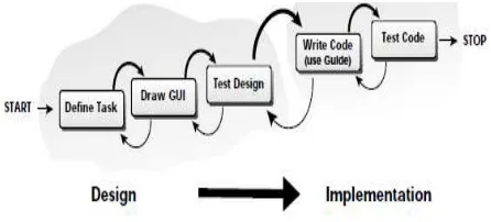
In all, the design and implementation of the MATLAB software was done using the MATLAB’s GUI development environment, also known as the M-GUIDE. The methodology used for the design and testing of the GUI is given in Figure 3.1.
Figure 3.1. GUI Design and Testing.
The useful specifications for the design of magnetic circuit of power transformer are listed in this section. They include:
1.Transformer Power rating, S in KVA 2.Frequency, f in Hz
3.Line voltage of the high voltage (HV) winding, Vinhv
4.Connection type – star or delta 5.Percentage impedance, Z%
6.Tapping on the H.V winding, Tp1, Tp2
3.1. Output Power Equation of Power Transfomer
In order to derive the equation for output power, S of power transformers, the equation for the induced voltage in the windings of the transformer will be derived first.
Suppose a coil of N-turns is wound on a core that is carrying a sinusoidal flux , then
Φ = ΦmSin2πft (3.1)
where Φm is the maximum flux density is Webbers, f is frequency in Hz, t is time in seconds, then the electromagnetic force (emf), e induced in the coil is given by Faraday’s law as [13]:
e = N(dΦ /dt) (3.2)
e = 2πΦmfN Cos(2πft) (3.3)
The maximum emf, Em is given from Equation 3.3 as
Em = 2πΦmfN (3.4)
The root mean square (rms) value of Em is given as
E= 4.44fΦmN (3.5)
Bm = Φm/Ai (3.6)
where, Ai is the cross sectional of the iron core area. Hence,
Φm = BmAi (3.7)
Substituting Φm into Equation3.5 gives
E= 4.44f BmAi N ( 3.8)
The voltage per turn, Vt is given as E/N. Thus from equation 3.8
Vt =4.44f BmAi (3.9)
Thus from equation 3.5
Vt =4.44fΦm (3.10)
Thus, from equation 3.9
Ai = Vt/ 4.44fBm (3.11)
For 3-phase each core window contains two sections of high voltage (HV) coils and two sections of low voltage (LV) coils [13, 14]. If Nphv and Nplv are the numbers of turns per phase and ahv and alv are the cross sectional areas of each conductors per window, then the total copper area per window is given by;
Total copper area per window = 2(Nphv ahv + Nplv alv) (3.12) The current density J is the same in both HV and LV coils. Thus,
J = Iplv/ alv (3.13a)
J = Iphv/ ahv (3.13b)
J = Ip/a (3.13c)
where Iphv and Iplv are phase current in the high voltage and low voltage side. Also, recall that for transformers
Vplv/Vphv = Nlv/Nhv = Iphv/Iplv
Thus,
Iplv Nlv = Iphv Nhv = IpN (3.14)
From equations 3.13a, 3.13b, and 3.13c, Iphv = ahv/J, Iplv = alv/J, Ip = a/J. Hence substituting Iphv, Iplv and Ip in equation 3.14, gives
Nlvalv/J = Nhv ahv/J = Na/J (3.15)
Hence, Nlvalv = Nhv ahv = Na (3.16)
Substituting for Nlv alv from Equation 3.16 into Equation 3.12 gives
Total copper area per window= 4 Nhv ahv (3.17)
Putting in general terms, whether it is LV or HV value
Total copper area per window = 4 Na (3.18)
Let Kw stand for window space factor where ;
Kw = ,
Kw = 4aN/Aw (3.19)
From equation 3.13c, a = Ip/J
So equation 3.19 becomes 4IpN/J = KwAw
IN = (KwAwJ)/4 (3.20)
For 3-phase transformer, S =3EI× 10-3 (3.21)
Substituting equation 3.8 into equation 3.21 gives
S=3.33fBmAiAmJKw× 10-3 (3.22)
For single phase transformers,
IN= (KwAwJ)/2 (3.23)
Thus,
S1-phase= 2.22fBmAiAwJKw × 10-3 (3.24)
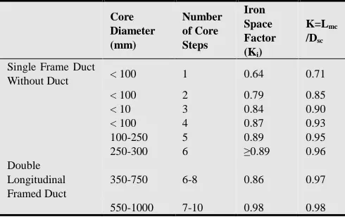
The power rating (in KVA) can also be expressed in terms of magnetic potential gradient. If Dsc is the diameter of the circumscribing circle for the core limb, then the area of the iron Ai is then given as
Ai = kiksπDsc2/4 (3.25)
where the Ks is stacking factor, Ki is the iron space factor given in Table 3.1.
Table 3.1. Iron Space Factor (Ki) and K (The Ratio Of The Diameter Of The Circumscribing Circle To The Maximum Core Limb Length For Various Core Steps).
Core Diameter (mm)
Number of Core Steps
Iron Space Factor (Ki)
K=Lmc /Dsc
Single Frame Duct
Without Duct < 100 1 0.64 0.71
< 100 2 0.79 0.85
< 10 3 0.84 0.90
< 100 4 0.87 0.93
100-250 5 0.89 0.95
250-300 6 ≥0.89 0.96
Double Longitudinal Framed Duct
350-750 6-8 0.86 0.97
550-1000 7-10 0.98 0.98
Now, the magnetic potential gradient, Hm is given as
Hm = (3.26)
Then for a 3-phase transformer, the total magneto motive force, mmf over one limb is given as
mmf = 2NI (3.27)
NI = HmHlmb/2 (3.28)
Putting Eq 3.28 into equation Eq 3.24 gives
S= 5.23fBm Dsc2 HmHlmbkiks × 10-3 (3.29)
For single phase transformer, mmf = NI. Thus
S1-phase= 3.48fBm Dsc2 H
mHlmbkiks × 10-3 (3.30)
3.2. The Core Dimensions
Power transformer cores are built of thin strips of laminations arranged in a number of steps so as to obtain nearly round cross sectional area so that better space factor for accommodating iron in the most useful ways can be achieved. The numbers of steps usually chosen are 3, 4,5,6,7 or 9 [13, 14]. The iron core area, Ai is given in Equation
3.25.It is expressed with respect to Dsc, ki and ks. The value
of Ai for various core steps can be obtained from table 3.1
above.
Ki, the iron space factor is there because of the use of steps
of iron instead of one solid round section of iron core. Ks is
due to paper or vanish insulation between the laminations of the core.
Dsc = √4Ai/πkiks (3.31)
ks= 0.92 for all steps of core. The maximum length of the
core limb, Lmc is given in table… for various core steps. It is
expressed with respect to Dsc in the form
Lmc= k(Dsc) (3.32)
Where k is the factor relating Lmc to Dsc. The value of k is
given in table 3.1 for the various core steps.
3.2.1. Core Yoke Dimensions
The flux in the core limb is the same as the flux in the yoke [13, 14] Hence, from Equation (3.32)
Blmb Almb = Byk Ayk (3.33)
Where Blmb and Byk are the flux density of the limb and
yoke, Almb and Ayk are the cross sectional area of the limb
and yoke respectively. Note that BImb = Bm and Aimb = Ai.
Then from Equation (3.33)
Ayk = Ai (Bm / Byk) (3.34)
In practice, Byk Bm. Empirical values for Byk can be
chosen from the relation 1 Bm / Byk ≤ 1.25. Put another
way Bm / 1.25 Byk 1.
The diameter of the circumscribing circle for the core yoke is given as in Equation (3.31)
Dsyk = % 4 Ayk / +kiks (3.35)
Similarly, the maximum length of the yoke, lmy is given as
in Equation (3.32)
Lmy = k (Dsyk) (3.36)
Where k, ki and ks are the same as the ones used for the
core in Equations (3.31) and (3.32)
3.2.2. The Core Window Dimensions
From Equation (3.22), the core window area, Aw is given
as
Aw = S/ ((3.33 fBm Ai J Kw) x 10-3) (3.37)
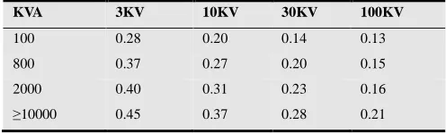
Table 3.2 gives the window space factor, kw. With kw
selected from Table 3.2 and the value of current density, J chosen, Aw can be computed from Equation (3.37). In
practice, the ratio of the window Height, Hw to the window
width, Ww is between 2 and 4. If Rhw represent the ratio of
Hw to Ww , then
Rhw = Hw /Ww (3.38)
It means from the statement above that 2 ≤ Rhw≤ 4
Table 3.2. Window Space Factor, Kw, Balbir, (1982).
KVA 3KV 10KV 30KV 100KV
100 0.28 0.20 0.14 0.13
800 0.37 0.27 0.20 0.15
2000 0.40 0.31 0.23 0.16
≥10000 0.45 0.37 0.28 0.21
However, values of Rhw beyond this range can be used,
from Equation (3.38)
Hw = Rhw Ww (3.39)
Now Aw = Hw Ww (3.40)
Thus Aw = Rhw Ww2 (3.41)
Hence, Ww = √ (Aw/Rhw) (3.42)
3.2.3. The overall Core Frame Dimension
Overall core frame height, H is given as
H=Hw+2Lmy (3.43)
The center –to-center distance, Dcc is given as:
Dcc = Ww +Dsc (3.44)
The overall core width
W = 2Dcc + Lmc (3.45)
3.2.4. Weight of the Core
The volume of iron core can be found from the product Ai.Lmf , where Lmf is the mean flux path including the core
limb and yokes. For single phase transformers
Lmf = 2(Ww +Dlmb)= 2 (Hw +Wlmb) (3.46)
For 3-phase transformers,
Lmf = 2(2Ww + 2 Dlmb)= 3(Hw +Wlmb) (3.47)
circle for the core limb cross section, Hw is the window
height. The volume of iron, Vi is given as
Vi = Ai.Lmf (3.48)
If the density of the iron core in cm3/kg is Pic, then weight
of iron, Wi is given as
Wi = Vi Pic (3.49)
3.3. Weight of the Copper
If Ephv and Eplv are the phase voltages of the H.V and L.V
winding respectively, then
Nhv = Ephv/Vt (3.50)
Niv = Eplv/Vt (3.51)
Note, for star connection, phase voltage is given as (line voltage/ √3).
To calculate the weight of copper, an approximate value can be obtained from the conductor cross sectional area and the mean length of turns, Lmf. Assuming that the window
space is completely filled with oil, we can allocate half of the window space to coils on each core limb. The mean diameter of the coil Dmt is therefore given as [14]
Dmt = Dlmb +Ww/2 (3.52)
Since Dlmb = Dsc
∴ Dmt = Dsc + Ww /2 (3.53)
∴ Lmt = π Dmt (3.54)
The volume of copper Vcp is given as
Vcp = Kw Lmt (Ww/2)Hw (3.55)
Where Kw is the window space factor. If ρcp is the density
of copper, then weight of copper Wcp is given as
Wcp = Vcpρcp (3.56)
3.4. Empirical Formula for Voltage Per Turn, Vt
In the design of a transformer, the value of voltage per turn, Vt is often needed to be chosen or calculated quite
fairly from the available parameters. The value of Vt so
chosen affects the size and weight of the transformer as well as other performance characteristics of the transformer Experts have proffered some empirical formula for Vt. Two
of the formula will be discussed here. Suppose we define
r = (Magnetic Loading)/Electric Loading)
Where Magnetic Loading = Фm and Electric Loading =
IN
∴ r = Фm/IN (3.57)
Thus, IN = Фm/r and from Equation (3.10), Vt = 4.44f Фm
Also from Equation (3.21), S = 3EI x 10-3 and E = Vt N.
Hence,
S = (4.44f Фm NI) x 10-3 (3.58)
Putting IN = Фm/r into Equation (3.58) gives
S = 4.44 f (Фm2/r) x 10-3 (3.59)
∴Фm = % S. r / 4.44f × 1045 (3.60)
Putting Фm from Equation (3.60) into Vt = 4.44f Фm gives
Vt = (4.44f) % S. r / 4.44f × 1045 (3.61)
∴ Vt = √ ((4.44f) (r) x10-3)(3.62)
If we define C = % 4.44f r x 1045 ,
∴Vt = C √S (3.63)
Where, S is the power rating in KVA. From Equation (3.63),
C = Vt /√S (3.64)
3.4.1. Significance of C
From C = % 4.44f r x 1045 , C is proportional to r. Also, from Equation (3.58) r is proportional to Фm. As such,
C is proportional to Фm and hence an increase in C will result
to increase Фm, if other variable remain constant.
Now, Фm = BmAi. If Bm is kept constant increasing Фm will
result to increase in Ai, which is the amount of iron used in
the transformer. On the other hand, N, the number of turns indicates the amount of copper used in the transformer. For any given e, (E = 4.44 f N Фm) and for a particular S, if Фm is
decreased, N will increase. So it will be observed that increasing the value of C will increase the amount of iron (Ai)
used and decrease N, the number of turns of copper. On the other hand decreasing the value of C will decrease the amount of iron (Ai) used and increase N. Therefore, C is a
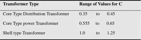
constant that indicates the amount of iron, Ai used and the number of turns, N, of the transformer. Table 3.3 below gives the average values that are usually used in practice for C [13, 14]
Table 3.3. Empirical Average Values For The Factor C.
Transformer Type Range of Values for C
Core Type Distribution Transformer 0.35 to 0.45
Core Type power Transformer 0.555 to 0.65
Shell type Transformer 1.0 to 1.25
3.4.2 . Second Empirical Formula for Vt
Another empirical formula for Vt is given as Bilbir, (1982)
Vt = (1/40) √ ((Sx1000) / Number of Legs) (3.64)
3.5. Algorithm for Designing the Magnetic Circuit of 3-Phase Power Transformer
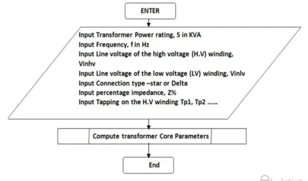
3.5.1. Design Specifications
Obtain the value of the following parameters from the given design specifications
1. Transformer Power rating, S, in kVA 2. Frequency, f in Hz
3. Line voltage of the high voltage (H.V) Winding, Vinhv
4. Line voltage of the low voltage (L.V) Winding, Vinlv
5. Connection type – star or Delta 6. Percentage impedance, Z%
7. Tapping on the H.V winding, Tp1, Tp2…
3.5.2 . Core Parameters
1. Compute volt per turn, Vt from Vt = C√ S or Vt = (1/40)
√ ((Sx1000) / Number of Legs)
2. Compute cross sectional area of core, Ai from Ai = Vt/
4.44fBm
3. Select window space factor from Table 3.2 4. Choose value for current density, J
5. Compute window area Aw from Aw = S/ ((3.33 fBm Ai J
Kw) x 10-3)
6. Select suitable ration for window height to window width from 2 ≤ Rhw≤ 4
7. Compute window area, Ww from Ww = √ (Aw/Rhw)
8. Compute window height, Hw from Hw = Rhw Ww
9. Choose number of steps for the Core 10. Choose iron space factor, Ki from Table 3.1
11. Choose stacking factor ks = 0.92
12. Choose diameter of circumscribing circle of Core limb, Dsc
13. Select K from Table 3.1 for the chosen number of steps in core
14. Compute maximum length of core, Lmc from Lmc= k
(Dsc)
15. Choose flux density of the yoke, Byk from 1≤ Bm / Byk
≤ 1.25
16. Compute diameter of circumscribing circle of yoke, Dsyk from
Dsyk = % 4 Ayk / +kiks
17. Compute maximum length of yoke Lmy from Lmy = k
(Dsyk)
18. Compute center –to center distance of limb, Dcc from
Dcc = Ww +Dsc
19. Compute overall core width, W from W = 2Dcc + Lmc
20. Compute overall core height, H from H=Hw+2Lmy
21. Compute mean length of flux path, Lmf from Lmf =
2(2Ww + 2 Dsc)
22. Compute the volume of iron, Vi from Vi = Ai.Lmf
23. Compute the weight of iron, Wi from Wi = Vi Pic
24. Compute number of turns in H.V winding, Nhv from
Nhv = Ephv/Vt
25. Compute number of turns in L.V winding, Nlv from
Nlv = Eplv/Vt
26. Compute mean diameter of the coil, Dmt from Dmt =
Dsc + Ww /2
27. Compute mean diameter length of turn, Lmt from Lmt =
π Dmt
28. Compute volume of copper, Vcp from Vcp = Kw Lmt
(Ww/2)Hw
29. Compute weight of copper wcp from Wcp = Vcpρcp
The flowchart for the design of the magnetic circuit of 3-phase power transformer is shown in Figure 3.2
Figure 3.2. Flowchart for the Design of the Magnetic Circuit of 3-Phase Power Transformer.
4. Results and Discussions
After coding, the MATLAB-based program was tested with a sample power transformer design. The design input and the results obtained are shown in the various screenshot of the program user interfaces. The sample design problem is as follows:
Design the electric circuit for a 8000kVA 3-phase, 50Hz, 220kV/11kV, delta/delta connected power transformer; construction- core, cooling-OFAF, temperature rise of oil 50oC, percentage impedance 11.5%. The transformer is provided with tapping ±2.5%, ±5% on the high voltage (HV) windings. The voltage per turn is 40, Ai = mm
2
W= mm, H = mm, Dsc = mm, where H is the overall frame height, W is
overall frame width and Dsc is the diameter of
circumscribing circle.
4.1. The Input Specification Module
The input specification module for the electric circuit parameters of power transformer consists of the input interfaces used to capture transformer input data and to process the data as shown in Fig 4.1
4.2. The Input Preview Module
The input preview module Fig 4.2 renders supplied input data from the input specification module with no editable field on its own. It provides the user option to either proceed with computation or return to input specification module for correction.
4.3. The Output Module
4.3.1. Tabular Output
obtained from calculations made by the design software. The results are displayed in tabular format (Fig 4.3). The design output interface also has option to proceed and plot a graphical view of the sample design output (shown in Fig 4.4); option to return to compute new data, option to close application and option for printing the design result.
Figure 4.1. Screenshot of the Input Specification Module.
Figure 4.2. Screenshot of the Input Preview Module.
Fig 4.3. Screenshot of the Design Output Interface Showing the Sample Design Results Displayed in Tabular Format.
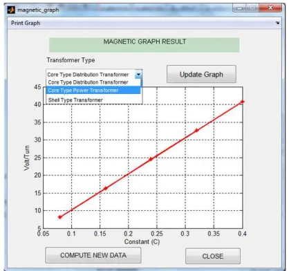
4.3.2. Graphical Output
Fig 4.4 presents result obtained for graphical output interface of the Matlab-based software for designing power transformer.
Fig 4.4. Plot of Volt Per Turn (Vt) vs Constant, C for a given transformer
Power Rating, S.
4.4. Discussion of Results
The output in Fig 4.2 and Fig 4.3 show that for the given power rating, S = 8000kVA, and Volt per Turn (Vt) of
40.82KV, the amount of iron (Ai) used is 114934.7 sq.mm
and the number of turns for the high voltage and for the
low voltage windings are 5.38 and 1.27 respectively. In addition, from the graph plot of Fig 4.4, it can be seen that for any given power rating S of the power transformer, the Vt
is proportional to the constant C. This result is in line with Eq 3.64 which states that C = Vt /√S. With the aid of the
Matlab program, it can also be demonstrated that, for any given C, increasing S, will increase Vt according to the
relationship, Vt = C (√S). Similarly, other useful
relationships among the transformer parameters can be easily demonstrated using the Matlab program. In particular, given that C is a constant that indicates the amount of iron, Ai used and the number of turns, N, of the transformer, hence,
it can be demonstrated with the Matlab program that if other variables remain constant, increasing the value of C will increase the amount of iron (Ai) used and decrease N, the
number of turns of copper.
5. Conclusion and Recommendation
5.1. Conclusion
developed and then a sample design problem was used to demonstrate how the program can be used. The simplicity of the mathematical models and the modular nature of the program make them relevant for teaching and hands-on training on power transformer design. It is also easy to upgrade the programs to accommodate the design of other kinds of transformers and the use of other design methodologies and also for incorporating optimization issues in the program.
5.2 Recommendation for further Works
The scope of this paper covers only the design of the electric circuit of 3-phase power transformers. In particular, the design considered disc winding with rectangular conductors only. Further work is needed to cover other types of transformers and other form of winding layouts and conductor shapes. Also, design optimization was not considered in this paper. However, the modular nature of the program makes provision for the program to be easily upgraded to include the optimization module. Consequently, further work is required to develop the mathematical models and program codes for those additional modules.
References
[1] Amoiralis, E. I., Tsili, M. A., & Kladas, A. G. (2009). Transformer design and optimization: a literature survey. Power Delivery, IEEE Transactions on, 24(4), 1999-2024.
[2] Amoiralis, E. I., Tsili, M. A., and Georgilakis, P. S. (2008). The state of the art in engineering methods for transformer design and optimization: a survey. Journal of Optoelectronics and Advanced Materials, 10(5), 1149.
[3] IEEE (2002) IEEE Standard Terminology for Power and
Distribution Transformers, IEEE Std C57.12.80-2002.
[4] Mittle VN, Mittal A (1996) Design of electrical machines, 4th edn. Standard Publishers Distributors, Nai Sarak, Delhi
[5] Amoiralis. E. I., Georgilakis. P. S., Tsili. M. A., Kladas A.G.and Souflaris A. T. (2011) A complete software package for transformer design optimization and economic evaluation analysis . Materials Science Forum Vol. 670 (2011) pp 535-546) Trans Tech Publications, Switzerland
[6] Judd F. F., Kressler D. R. (1977), IEEE Trans. Magn., vol. MAG-13, pp. 1058-1069.
[7] Poloujadoff M., Findlay R. D. (1986), IEEE Trans. Power Sys., vol. PWRS-1.
[8] Jewell W. T. (1990) IEEE Trans. Power Sys., vol. 5 , pp. 499-505.
[9] Grady W. M., Chan R., Samotyj M. J., Ferraro R. J., Bierschenk J. L. (1992) IEEE Trans. Power Sys.,vol. 7 (1992), pp. 709-717.
[10] Rubaai A. (11994), IEEE Trans. Power Sys., vol. 9 , pp. 1174-1181.
[11] Andersen O. W(1991), IEEE Comput. Appl. Power, vol.
4 ,pp. 11–15.
[12] Hernandez C., Arjona M. A., Shi-Hai Dong (2008) IEEE Trans. Magn., vol. 44 , pp. 2332-2337.
[13] Ozuomba, S. et al (2004) “Software Development for the Design of Electric Circuit of 3-Phase Power Transformer” University of Uyo - A draft paper
[14] Oboma, S. O (2003) Development of Computer Program for