Distributed Matrix Completion and Robust Factorization
Lester Mackey† [email protected]
Stanford University Department of Statistics 390 Serra Mall
Stanford, CA 94305
Ameet Talwalkar† [email protected]
University of California, Los Angeles Computer Science Department 4732 Boelter Hall
Los Angeles, CA 90095
Michael I. Jordan [email protected] University of California, Berkeley
Department of Electrical Engineering and Computer Science and Department of Statistics 465 Soda Hall
Berkeley, CA 94720
Editor:Nathan Srebro
† These authors contributed equally.
Abstract
If learning methods are to scale to the massive sizes of modern data sets, it is essential for the field of machine learning to embrace parallel and distributed computing. Inspired by the recent development of matrix factorization methods with rich theory but poor compu-tational complexity and by the relative ease of mapping matrices onto distributed architec-tures, we introduce a scalable divide-and-conquer framework for noisy matrix factorization. We present a thorough theoretical analysis of this framework in which we characterize the statistical errors introduced by the “divide” step and control their magnitude in the “con-quer” step, so that the overall algorithm enjoys high-probability estimation guarantees comparable to those of its base algorithm. We also present experiments in collaborative filtering and video background modeling that demonstrate the near-linear to superlinear speed-ups attainable with this approach.
Keywords: collaborative filtering, divide-and-conquer, matrix completion, matrix torization, parallel and distributed algorithms, randomized algorithms, robust matrix fac-torization, video surveillance
1. Introduction
because of the statistical strength of the data. While this is a reasonable research strategy, it requires developing suites of algorithms of varying computational complexity for each inferential task and calibrating statistical and computational efficiencies. There are many open problems that need to be solved if such an effort is to bear fruit.
The other response to the massive data problem is to retain existing algorithms but to apply them to subsets of the data. To obtain useful results under this approach, one em-braces parallel and distributed computing architectures, applying existing base algorithms to multiple subsets of the data in parallel and then combining the results. Such a divide-and-conquer methodology has two main virtues: (1) it builds directly on algorithms that have proven their value at smaller scales and that often have strong theoretical guarantees, and (2) it requires little in the way of new algorithmic development. The major challenge, however, is in preserving the theoretical guarantees of the base algorithm once one em-beds the algorithm in a computationally-motivated divide-and-conquer procedure. Indeed, the theoretical guarantees often refer to subtle statistical properties of the data-generating mechanism (e.g., sparsity, information spread, and near low-rankedness). These may or may not be retained under the “divide” step of a putative divide-and-conquer solution. In fact, we generally would expect subsampling operations to damage the relevant statisti-cal structures. Even if these properties are preserved, we face the difficulty of combining the intermediary results of the “divide” step into a final consilient solution to the original problem. The question, therefore, is whether we can design divide-and-conquer algorithms that manage the tradeoffs relating these statistical properties to the computational degrees of freedom such that the overall algorithm provides a scalable solution that retains the theoretical guarantees of the base algorithm.
In this paper,1 we explore this issue in the context of an important class of machine learning algorithms—the matrix factorization algorithms underlying a wide variety of prac-tical applications, including collaborative filtering for recommender systems , e.g., Koren et al. (2009) and the references therein, link prediction for social networks (Hoff, 2005), click prediction for web search (Das et al., 2007), video surveillance (Cand`es et al., 2011), graphical model selection (Chandrasekaran et al., 2009), document modeling (Min et al., 2010), and image alignment (Peng et al., 2010). We focus on two instances of the general matrix factorization problem: noisy matrix completion (Cand`es and Plan, 2010), where the goal is to recover a low-rank matrix from a small subset of noisy entries, and noisy robust matrix factorization (Cand`es et al., 2011; Chandrasekaran et al., 2009), where the aim is to recover a low-rank matrix from corruption by noise and outliers of arbitrary magnitude. These two classes of matrix factorization problems have attracted significant interest in the research community.
Various approaches have been proposed for scalable noisy matrix factorization prob-lems, in particular for noisy matrix completion, though the vast majority tackle rank-constrained non-convex formulations of these problems with no assurance of finding optimal solutions (Zhou et al., 2008; Gemulla et al., 2011; Recht and R´e, 2011; F. Niu et al., 2011; Yu et al., 2012). In contrast, convex formulations of noisy matrix factorization relying on the nuclear norm have been shown to admit strong theoretical estimation guarantees (Agarwal et al., 2011; Cand`es et al., 2011; Cand`es and Plan, 2010; Negahban and Wainwright, 2012),
and a variety of algorithms (e.g., Lin et al., 2009b; Ma et al., 2011; Toh and Yun, 2010) have been developed for solving both matrix completion and robust matrix factorization via con-vex relaxation. Unfortunately, however, all of these methods are inherently sequential, and all rely on the repeated and costly computation of truncated singular value decompositions (SVDs), factors that severely limit the scalability of the algorithms. Moreover, previous attempts at reducing this computational burden have introduced approximations without theoretical justification (Mu et al., 2011).
To address this key problem of noisy matrix factorization in a scalable and theoret-ically sound manner, we propose a divide-and-conquer framework for large-scale matrix factorization. Our framework, entitled Divide-Factor-Combine (DFC), randomly divides
the original matrix factorization task into cheaper subproblems, solves those subproblems in parallel using a base matrix factorization algorithm for nuclear norm regularized for-mulations, and combines the solutions to the subproblems using efficient techniques from randomized matrix approximation. We develop a thoroughgoing theoretical analysis for the
DFC framework, linking statistical properties of the underlying matrix to computational
choices in the algorithms and thereby providing conditions under which statistical estima-tion of the underlying matrix is possible. We also present experimental results for several
DFCvariants demonstrating thatDFCcan provide near-linear to superlinear speed-ups in
practice. Indeed, DFC naturally handles massive data sets that are too large to fit on a single machine, as DFC’s minimal communication footprint is particularly well-suited for
distributed computing environments.
The remainder of the paper is organized as follows. In Section 2, we define the setting of noisy matrix factorization and introduce the components of theDFC framework. Secs. 3,
4, and 5 present our theoretical analysis of DFC, along with a new analysis of convex
noisy matrix completion and a novel characterization of randomized matrix approximation algorithms. To illustrate the practical speed-up and robustness of DFC, we present
exper-imental results on collaborative filtering, video background modeling, and simulated data in Section 6. Finally, we conclude in Section 7.
Notation: For a matrixM∈Rm×n, we defineM
(i)as theith row vector,M(j)as thejth column vector, and Mij as the ijth entry. If rank(M) = r, we write the compact singular value decomposition (SVD) of M as UMΣMVM>, whereΣM is diagonal and contains the
r non-zero singular values ofM, and UM ∈Rm×r and VM ∈Rn×r are the corresponding left and right singular vectors of M. We define M+ =VMΣ−1MU>M as the Moore-Penrose pseudoinverse ofM and PM =MM+ as the orthogonal projection onto the column space of M. We letk·k2, k·kF, and k·k∗ respectively denote the spectral, Frobenius, and nuclear norms of a matrix, k·k∞ denote the maximum entry of a matrix, andk·k represent the `2 norm of a vector.
2. The Divide-Factor-Combine Framework
2.1 Noisy Matrix Factorization (MF)
In the setting of noisy matrix factorization, we observe a subset of the entries of a matrix M =L0+S0 +Z0 ∈ Rm×n, where L0 has rank r m, n, S0 represents a sparse matrix of outliers of arbitrary magnitude, and Z0 is a dense noise matrix. We let Ω represent the locations of the observed entries and PΩ be the orthogonal projection onto the space of
m×n matrices with support Ω, so that
(PΩ(M))ij =Mij, if (i, j)∈Ω and (PΩ(M))ij = 0 otherwise.2
Our goal is to estimate the low-rank matrixL0 fromPΩ(M) with error proportional to the noise level ∆,kZ0kF. We will focus on two specific instances of this general problem:
• Noisy Matrix Completion (MC): s , |Ω| entries of M are revealed uniformly without replacement, along with their locations. There are no outliers, so that S0 is identically zero.
• Noisy Robust Matrix Factorization (RMF): S0 is identically zero save for s outlier entries of arbitrary magnitude with unknown locations distributed uniformly without replacement. All entries ofM are observed, so that PΩ(M) =M.
2.2 Divide-Factor-Combine
The Divide-Factor-Combine (DFC) framework divides the expensive task of matrix factor-ization into smaller subproblems, executes those subproblems in parallel, and then efficiently combines the results into a final low-rank estimate ofL0. We highlight three variants of this general framework in Algorithms 1, 2, and 3. These algorithms, which we refer to as DFC-Proj, DFC-RP, and DFC-Nys, differ in their strategies for division and recombination
but adhere to a common pattern of three simple steps:
(D step) Divide input matrix into submatrices: DFC-ProjandDFC-RPrandomly
partition PΩ(M) into t l-column submatrices, {PΩ(C1), . . . ,PΩ(Ct)},3 while
DFC-Nysselects anl-column submatrix,PΩ(C), and ad-row submatrix,PΩ(R), uniformly at random.
(F step) Factor each submatrix in parallel using any base MF algorithm:
DFC-Proj and DFC-RP perform t parallel submatrix factorizations, while DFC-Nys
performs two such parallel factorizations. Standard base MF algorithms output the following low-rank approximations: {C1ˆ , . . . ,Ctˆ } for DFC-Proj and DFC-RP; ˆC
and ˆRforDFC-Nys. All matrices are retained in factored form.
(C step) Combine submatrix estimates: DFC-Proj generates a final low-rank esti-mate ˆLproj by projecting [ ˆC1, . . . ,Ctˆ ] onto the column space of ˆC1, DFC-RP uses
random projection to compute a rank-kestimate ˆLrp of [ ˆC1· · ·Cˆt] wherekis the me-dian rank of the returned subproblem estimates, and DFC-Nysforms the low-rank
2. WhenQ is a submatrix of M we abuse notation and let PΩ(Q) be the corresponding submatrix of
PΩ(M).
Algorithm 1 DFC-Proj
Input: PΩ(M), t
{PΩ(Ci)}1≤i≤t =SampCol(PΩ(M),t) do in parallel
ˆ
C1 =Base-MF-Alg(PΩ(C1)) ..
. ˆ
Ct= Base-MF-Alg(PΩ(Ct)) end do
ˆ
Lproj = ColProjection( ˆC1, . . . ,Ctˆ )
Algorithm 2 DFC-RP
Input: PΩ(M), t
{PΩ(Ci)}1≤i≤t =SampCol(PΩ(M),t) do in parallel
ˆ
C1 =Base-MF-Alg(PΩ(C1)) ..
. ˆ
Ct= Base-MF-Alg(PΩ(Ct)) end do
k= mediani∈{1...t} rank( ˆCi)
ˆ
Lproj = RandProjection( ˆC1, . . . ,Cˆt, k)
Algorithm 3 DFC-Nys
Input: PΩ(M), l,d
PΩ(C),PΩ(R) =SampColRow(PΩ(M),l,d) do in parallel
ˆ
C=Base-MF-Alg(PΩ(C)) ˆ
R =Base-MF-Alg(PΩ(R)) end do
ˆ
Lnys =GenNystr¨om( ˆC, ˆR)
estimate ˆLnys from ˆC and ˆR via the generalized Nystr¨om method. These matrix approximation techniques are described in more detail in Section 2.3.
2.3 Randomized Matrix Approximations
Underlying the C step of each DFC algorithm is a method for generating randomized low-rank approximations to an arbitrary matrixM.
Column Projection: DFC-Proj (Algorithm 1) uses the column projection method of
Frieze et al. (1998). Suppose that C is a matrix of l columns sampled uniformly and without replacement from the columns ofM. Then, column projection generates a “matrix projection” approximation (Kumar et al., 2009a) of Mvia
Lproj =CC+M=UCU>CM.
In practice, we do not reconstructLproj but rather maintain low-rank factors, e.g.,UC and U>CM.
Random Projection: The celebrated result of Johnson and Lindenstrauss (1984) shows that random low-dimensional embeddings preserve Euclidean geometry. Inspired by this result, several random projection algorithms (e.g., Papadimitriou et al., 1998; Liberty, 2009; Rokhlin et al., 2009) have been introduced for approximating a matrix by projecting it onto a random low-dimensional subspace (see Halko et al. 2011 for further discussion). DFC-RP
target low-rank parameterk, let G be ann×(k+p) standard Gaussian matrixG, where
pis an oversampling parameter. Next, letY = (MM>)qMG, and defineQ∈Rm×k as the topk left singular vectors ofY. The random projection approximation of Mis then given by
Lrp =QQ+M.
We work with an implementation (Tygert, 2009) of a numerically stable variant of this algorithm described in Algorithm 4.4 of Halko et al. (2011). Moreover, the parameters p
and q are typically set to small positive constants (Tygert, 2009; Halko et al., 2011), and we set p= 5 and q = 2.
Generalized Nystr¨om Method: The Nystr¨om method was developed for the discretization of integral equations (Nystr¨om, 1930) and has since been used to speed up large-scale learn-ing applications involvlearn-ing symmetric positive semidefinite matrices (Williams and Seeger, 2000). DFC-Nys(Algorithm 3) makes use of a generalization of the Nystr¨om method for
arbitrary real matrices (Goreinov et al., 1997). Suppose thatCconsists oflcolumns of M, sampled uniformly without replacement, and thatRconsists ofdrows ofM, independently sampled uniformly and without replacement. LetWbe thed×lmatrix formed by sampling the corresponding rows ofC.4 Then, the generalized Nystr¨om method computes a “spectral reconstruction” approximation (Kumar et al., 2009a) ofM via
Lnys =CW+R=CVWΣ+WU>WR.
As withMproj, we store low-rank factors ofLnys, such asCVWΣ+W and U>WR.
Algorithm Factorization (Per Iteration) Combine Step
Serial Parallel Serial Parallel
Base Alg O(mnkˆ) O(mnkˆ) -
-DFC-Proj O(tmlˆk) O(mlˆk) O(tmˆk2) O(mˆk2)
DFC-RP O(tmlˆk) O(mlˆk) O(tmkˆ2+nˆk) O(mˆk2+tmkˆ+nkˆ)
DFC-Nys O((ml+nd)ˆk) O(max(ml, nd)ˆk) O(mˆk2) O(mˆk2)
Table 1: Summary of running time complexity of DFCvariants in contrast to many
stan-dard start-of-the-art MF algorithms. This running time analysis assumes that
l≤m≤nand that all low-rank matrices considered have rank ˆk. See Section 2.4 for a more detailed analysis.
2.4 Running Time of DFC
Many state-of-the-art MF algorithms have Ω(mnkM) per-iteration time complexity due to the rank-kM truncated SVD performed on each iteration. DFC significantly reduces the per-iteration complexity to O(mlkCi) time forCi(orC) and O(ndkR) time forR. The cost of combining the submatrix estimates is even smaller when using column projection or the generalized Nystr¨om method, since the outputs of standard MF algorithms are returned
in factored form. Indeed, if we define k0 , maxikCi, then the column projection step of
DFC-Projrequires only O(mk02+lk02) time: O(mk02+lk02) time for the pseudoinversion
of ˆC1 and O(mk02+lk02) time for matrix multiplication with each ˆCi in parallel. Similarly, the generalized Nystr¨om step of DFC-Nysrequires only O(lk¯2+d¯k2+ min(m, n)¯k2) time,
where ¯k,max(kC, kR).
DFC-RPalso benefits from the factored form of the outputs of standard MF algorithms. Assuming that p and q are positive constants, the random projection step of DFC-RP
requires O(mkt+mkk0+lkk0+nk) time where k is the low-rank parameter ofQ: O(nk) time to generate G, O(mkk0+lkk0+mkt) to compute Y in parallel, O(mk2) to compute the SVD of Y, and O(mk02+lk02) time for matrix multiplication with each ˆCi in parallel in the final projection step. Note that the running time of the random projection step depends on t (even when executed in parallel) and thus has a larger complexity than the column projection and generalized Nystr¨om variants. Nevertheless, the random projection step need be performed only once and thus yields a significant savings over the repeated computation of SVDs required by typical base algorithms.
A summary of these running times is presented in Table 1.
2.5 Ensemble Methods
Ensemble methods have been shown to improve performance of matrix approximation al-gorithms, while straightforwardly leveraging the parallelism of modern many-core and dis-tributed architectures (Kumar et al., 2009b). As such, we propose ensemble variants of theDFC algorithms that demonstrably reduce estimation error while introducing a
negli-gible cost to the parallel running time. For DFC-Proj-Ens, rather than projecting only
onto the column space of ˆC1, we project [ ˆC1, . . . ,Ctˆ ] onto the column space of each ˆCi in parallel and then average the t resulting low-rank approximations. For DFC-RP-Ens,
rather than projecting only onto a column space derived from a single random matrix G, we project [ ˆC1, . . . ,Ctˆ ] onto t column spaces derived from t random matrices in parallel and then average thetresulting low-rank approximations. ForDFC-Nys-Ens, we choose a
randomd-row submatrixPΩ(R) as in DFC-Nysand independently partition the columns
of PΩ(M) into {PΩ(C1), . . . ,PΩ(Ct)} as in DFC-Proj and DFC-RP. After running the
base MF algorithm on each submatrix, we apply the generalized Nystr¨om method to each ( ˆCi,Rˆ) pair in parallel and average the t resulting low-rank approximations. Section 6 highlights the empirical effectiveness of ensembling.
3. Roadmap of Theoretical Analysis
WhileDFCin principle can work with any base matrix factorization algorithm, it offers the
improve the scalability of these algorithms, but we first present a thorough theoretical analysis of the estimation properties of DFC.
Over the course of the next three sections, we will show that the same assumptions that give rise to strong estimation guarantees for standard MF formulations also guarantee strong estimation properties forDFC. While these results represent an important first step
toward understanding the theoretical behavior of DFC, we will see that certain gaps remain
between our theoretical characterization and the practical performance of DFC. We will
reflect on these gaps and the attendant opportunities for tightened theoretical analysis in Section 6.4. In the remainder of this section, we first introduce these standard assumptions and then present simplified bounds to build intuition for our theoretical results and our underlying proof techniques.
3.1 Standard Assumptions for Noisy Matrix Factorization
Since not all matrices can be recovered from missing entries or gross outliers, recent theo-retical advances have studied sufficient conditions for accurate noisy MC (Cand`es and Plan, 2010; Keshavan et al., 2010; Negahban and Wainwright, 2012) and RMF (Agarwal et al., 2011; Zhou et al., 2010). Informally, these conditions capture the degree to which informa-tion about a single entry is “spread out” across a matrix. The ease of matrix estimainforma-tion is correlated with this spread of information. The most prevalent set of conditions arematrix coherence conditions, which limit the extent to which the singular vectors of a matrix are correlated with the standard basis. However, there exist classes of matrices that violate the coherence conditions but can nonetheless be recovered from missing entries or gross outliers. Negahban and Wainwright (2012) define an alternative notion of matrix spikiness in part to handle these classes.
3.1.1 Matrix Coherence
Letting ei be the ith column of the standard basis, we define two standard notions of coherence (Recht, 2011):
Definition 1 (µ0-Coherence) Let V ∈ Rn×r contain orthonormal columns with r ≤ n.
Then the µ0-coherence of V is:
µ0(V), nr max1≤i≤nkPVeik2= nrmax1≤i≤nkV(i)k2.
Definition 2 (µ1-Coherence) Let L ∈ Rm×n have rank r. Then, the µ1-coherence of L
is:
µ1(L),
pmn
r maxij|e >
i ULVL>ej|.
For conciseness, we extend the definition ofµ0-coherence to an arbitrary matrixL∈Rm×n with rankrviaµ0(L),max(µ0(UL), µ0(VL)).Further, for anyµ >0, we will call a matrix L (µ, r)-coherent if rank(L) = r, µ0(L) ≤ µ, and µ1(L) ≤
√
3.1.2 Matrix Spikiness
The matrix spikiness condition of Negahban and Wainwright (2012) captures the intuition that a matrix is easier to estimate if its maximum entry is not much larger than its average entry (in the root mean square sense):
Definition 3 (Spikiness) The spikiness of L∈Rm×n is:
α(L),√mnkLk∞/kLkF.
We call a matrix α-spiky if α(L)≤α.
Our analysis in Section 5 will focus on base MC algorithms that express their estimation guarantees in terms of theα-spikiness of the target low-rank matrixL0. For such algorithms, lower values ofα correspond to better estimation properties.
3.2 Prototypical Estimation Bounds
We now present a prototypical estimation bound forDFC. Suppose that a base MC
algo-rithm solves thenoisy nuclear norm heuristic, studied in Cand`es and Plan (2010):
minimizeL kLk∗ subject to kPΩ(M−L)kF ≤∆,
and that, for simplicity, M is square. The following prototype bound, derived from a new noisy MC guarantee in Theorem 10, describes the behavior of this estimator under matrix coherence assumptions. Note that the bound implies exact recovery in the noiseless setting, i.e., when ∆ = 0.
Proto-Bound 1 (MC under Incoherence) Suppose that L0 is (µ, r)-coherent, s en-tries of M ∈ Rn×n are observed uniformly at random where s = Ω(µrnlog2(n)), and kM−L0kF ≤∆. IfLˆ solves the noisy nuclear norm heuristic, then
kL0−LˆkF ≤f(n)∆
with high probability, where f is a function of n.
Now we present a corresponding prototype bound for DFC-Proj, a simplified version
of our Corollary 14, under precisely the same coherence assumptions. Notably, this bound i) preserves accuracy with a flexible (2 +) degradation in estimation error over the base algorithm, ii) allows for speed-up by requiring only a vanishingly small fraction of columns to be sampled (i.e., l/n → 0) whenever s = ω(nlog2(n)) entries are revealed, and iii) maintains exact recovery in the noiseless setting.
Proto-Bound 2 (DFC-MC under Incoherence) Suppose that L0 is (µ, r)-coherent, s
entries of M ∈ Rn×n are observed uniformly at random, and kM−L0kF ≤ ∆. Then it
suffices to choose
l≥cµ
2r2n2log2(n)
random columns suffice to have
kL0−LˆprojkF ≤(2 +)f(n)∆
with high probability when the noisy nuclear norm heuristic is used as a base algorithm, where f is the same function of n defined in Proto. 1 andc is a fixed positive constant.
The proof of Proto. 2, and indeed of each of our mainDFCresults, consists of three
high-level steps:
1. Bound coherence of submatrices: Recall that the F step of DFCoperates by applying
a base MF algorithm to submatrices. We show that, with high probability, uniformly sampled submatrices are only moderately more coherent and moderately more spiky than the matrix from which they are drawn. This allows for accurate estimation of submatrices using base algorithms with standard coherence or spikiness require-ments. The conservation of incoherence result is summarized in Lemma 4, while the conservation of non-spikiness is presented in Lemma 17.
2. Bound error of randomized matrix approximations: The error introduced by the C step of DFCdepends on the framework variant. Drawing upon tools from
random-ized `2 regression (Drineas et al., 2008), randomized matrix multiplication (Drineas et al., 2006a,b), and matrix concentration (Hsu et al., 2012), we show that the same assumptions on the spread of information responsible for accurate MC and RMF also yield high fidelity reconstructions for column projection (Corollary 6 and Theorem 18) and the Nystr¨om method (Corollary 7 and Corollary 8). We additionally present gen-eral approximation guarantees for random projection due to Halko et al. (2011) in Corollary 9. These results give rise to “master theorems” for coherence (Theorem 12) and spikiness (Theorem 20) that generically relate the estimation error of DFC to
the error of any base algorithm.
3. Bound error of submatrix factorizations: The final step combines a master theorem with a base estimation guarantee applied to each DFC subproblem. We study both
new (Theorem 10) and established bounds (Theorem 11 and Corollary 19) for MC and RMF and prove thatDFCsubmatrices satisfy the base guarantee preconditions with
high probability. We present the resulting coherence-based estimation guarantees for DFC in Corollary 14 and Corollary 16 and the spikiness-based estimation guarantee in Corollary 22.
The next two sections present the main results contributing to each of these proof steps, as well as their consequences for MC and RMF. Section 4 presents our analysis under coherence assumptions, while Section 5 contains our spikiness analysis.
4. Coherence-based Theoretical Analysis
This section presents our analysis of DFCunder standard coherence assumptions
4.1 Coherence Analysis of Randomized Approximation Algorithms
We begin our coherence-based analysis by characterizing the behavior of randomized ap-proximation algorithms under standard coherence assumptions. The derived properties will aid us in derivingDFCestimation guarantees. Hereafter, ∈(0,1] represents a prescribed
error tolerance, and δ, δ0∈(0,1] denote target failure probabilities.
4.1.1 Conservation of Incoherence
Our first result bounds theµ0 andµ1-coherence of a uniformly sampled submatrix in terms of the coherence of the full matrix. This conservation of incoherence allows for accurate submatrix completion or submatrix outlier removal when using standard MC and RMF algorithms. Its proof is given in Section B.
Lemma 4 (Conservation of Incoherence) LetL∈Rm×nbe a rank-rmatrix and define
LC ∈ Rm×l as a matrix of l columns of L sampled uniformly without replacement. If
l≥crµ0(VL) log(n) log(1/δ)/2, where c is a fixed positive constant defined in Corollary 6,
then
i) rank(LC) = rank(L)
ii) µ0(ULC) =µ0(UL) iii) µ0(VLC)≤
µ0(VL) 1−/2
iv) µ21(LC)≤
rµ0(UL)µ0(VL) 1−/2
all hold jointly with probability at least 1−δ/n.
4.1.2 Column Projection Analysis
Our next result shows that projection based on uniform column sampling leads to near optimal estimation in matrix regression when the covariate matrix has small coherence. This statement will immediately give rise to estimation guarantees for column projection and the generalized Nystr¨om method.
Theorem 5 (Subsampled Regression under Incoherence) Given a target matrixB∈ Rp×n and a rank-r matrix of covariates L∈Rm×n, choose l ≥3200rµ0(VL) log(4n/δ)/2,
let BC ∈Rp×l be a matrix of l columns of B sampled uniformly without replacement, and let LC ∈Rm×l consist of the corresponding columns of L. Then,
kB−BCL+CLkF ≤(1 +)kB−BL +Lk
F
with probability at least 1−δ−0.2.
randomized `2 regression work of Drineas et al. (2008) and the matrix concentration re-sults of Hsu et al. (2012) to yield a subsampled regression guarantee with better sampling complexity than that of Drineas et al. (2008, Theorem 5).
A first consequence of Theorem 5 shows that, with high probability, column projection produces an estimate nearly as good as a given rank-r target by sampling a number of columns proportional to the coherence and rlogn.
Corollary 6 (Column Projection under Incoherence) Given a matrix M ∈ Rm×n
and a rank-r approximation L∈Rm×n, choose l≥crµ0(VL) log(n) log(1/δ)/2, where c is
a fixed positive constant, and letC∈Rm×lbe a matrix oflcolumns ofMsampled uniformly without replacement. Then,
kM−CC+MkF ≤(1 +)kM−LkF with probability at least 1−δ.
Our result generalizes Theorem 1 of Drineas et al. (2008) by providing improved sampling complexity and guarantees relative to anarbitrarylow-rank approximation. Notably, in the “noiseless” setting, when M = L, Corollary 6 guarantees exact recovery of M with high probability. The proof of Corollary 6 is given in Section C.
4.1.3 Generalized Nystr¨om Analysis
Theorem 5 and Corollary 6 together imply an estimation guarantee for the generalized Nystr¨om method relative to an arbitrary low-rank approximation L. Indeed, if the ma-trix of sampled columns is denoted by C, then, with appropriately reduced probability, O(µ0(VL)rlogn) columns and O(µ0(UC)rlogm) rows suffice to match the reconstruction error of L up to any fixed precision. The proof can be found in Section D.
Corollary 7 (Generalized Nystr¨om under Incoherence) Given a matrixM∈Rm×n
and a rank-r approximation L ∈ Rm×n, choose l ≥ crµ0(VL) log(n) log(1/δ)/2 with c a
constant as in Corollary 6, and let C ∈ Rm×l be a matrix of l columns of M sampled uniformly without replacement. Further choose d ≥ clµ0(UC) log(m) log(1/δ0)/2, and let R ∈ Rd×n be a matrix of d rows of M sampled independently and uniformly without
re-placement. Then,
kM−CW+RkF ≤(1 +)2kM−LkF with probability at least (1−δ)(1−δ0−0.2).
Like the generalized Nystr¨om bound of Drineas et al. (2008, Theorem 4) and unlike our column projection result, Corollary 7 depends on the coherence of the submatrix C and holds only with probability bounded away from 1. Our next contribution shows that we can do away with these restrictions in the noiseless setting, whereM=L.
Corollary 8 (Noiseless Generalized Nystr¨om under Incoherence) Let L ∈ Rm×n
be a rank-rmatrix. Choosel≥48rµ0(VL) log(4n/(1− √
1−δ))andd≥48rµ0(UL) log(4m/(1− √
1−δ)). Let C∈Rm×l be a matrix of l columns ofL sampled uniformly without replace-ment, and let R ∈Rd×n be a matrix of d rows of L sampled independently and uniformly
without replacement. Then,
with probability at least 1−δ.
This result may appear surprising at first sight, since only vanishingly small fractions of rows and columns may participate in the generalized Nystr¨om reconstruction. The intuition for the method’s success that when the rank of L is small, only a small number of well-chosen rows and columns are needed to reconstruct the row and column space of L and that, when L is incoherent, uniform random sampling is likely produce well-chosen rows and columns. The proof of Corollary 8, given in Section E, adapts a strategy of Talwalkar and Rostamizadeh (2010) developed for the analysis of positive semidefinite matrices.
4.1.4 Random Projection Analysis
We next present an estimation guarantee for the random projection method relative to an arbitrary low-rank approximation L. The result implies that using a random matrix with oversampled columns proportional to rlog(1/δ) suffices to match the reconstruction error of Lup to any fixed precision with probability 1−δ. The result is a direct consequence of the random projection analysis of Halko et al. (2011, Theorem 10.7), and the proof can be found in Section F.
Corollary 9 (Random Projection) Given a matrix M ∈ Rm×n and a rank-r approxi-mation L∈Rm×n with r≥2, choose an oversampling parameter
p≥242 rlog(7/δ)/2.
Draw an n×(r +p) standard Gaussian matrix G and define Y = MG. Then, with probability at least 1−δ,
kM−PYMkF ≤(1 +)kM−LkF.
Moreover, defineLrp as the best rank-rapproximation ofPYMwith respect to the Frobenius
norm. Then, with probability at least 1−δ,
kM−LrpkF ≤(2 +)kM−LkF.
We note that, in contrast to Corollary 6 and Corollary 7, Corollary 9 does not depend on the coherence ofLand hence can be fruitfully applied even in the absence of an incoherence assumption. We demonstrate such a use case in Section 5. We note moreover that past empirical studies have demonstrated excellent estimation error with p≤10 irrespective of the target matrix rank (Halko et al., 2011); bridging the gap between theory and practice in this instance represents an interesting open problem.
4.2 Base Algorithm Guarantees
Theorem 10 (Noisy MC under Incoherence) Suppose thatL0∈Rm×nis(µ, r)-coherent
and that, for some target rate parameter β >1,
s≥32µr(m+n)βlog2(m+n)
entries of M are observed with locations Ω sampled uniformly without replacement. Then, if m≤n and kPΩ(M)− PΩ(L0)kF ≤∆a.s., the minimizer Lˆ of the problem
minimizeL kLk∗ subject to kPΩ(M−L)kF ≤∆. (1)
satisfies
kL0−LˆkF ≤8
r
2m2n
s +m+
1
16∆≤ce √
mn∆
with probability at least 1−4 log(n)n2−2β for ce a positive constant.
A similar estimation guarantee was obtained by Cand`es and Plan (2010) under stronger assumptions. We give the proof of Theorem 10 in Section J.
The second result, due to Zhou et al. (2010) and reformulated for a generic rate pa-rameterβ, as described in Cand`es et al. (2011, Section 3.1), bounds the estimation error of a convex optimization approach to noisy RMF, under the assumptions of incoherence and uniformly distributed outliers.
Theorem 11 (Noisy RMF under Incoherence, Zhou et al. 2010, Theorem 2) Suppose that L0 is (µ, r)-coherent and that the support set of S0 is uniformly distributed among all
sets of cardinality s. Then, if m≤n and kM−L0−S0kF ≤∆ a.s., there is a constant cp
such that with probability at least 1−cpn−β, the minimizer ( ˆL,Sˆ) of the problem
minimizeL,S kLk∗+λkSk1 subject to kM−L−SkF ≤∆ with λ= 1/ √
n (2)
satisfieskL0−Lˆk 2
F +kS0−Sˆk 2
F ≤c02emn∆2, provided that
r≤ ρrm
µlog2(n) and s≤(1−ρsβ)mn for target rate parameter β >2, and positive constantsρr, ρs,and c0e. 4.3 Coherence Master Theorem
We now show that the same coherence conditions that allow for accurate MC and RMF also imply high-probability estimation guarantees for DFC. To make this precise, we let
M =L0 +S0+Z0 ∈ Rm×n, where L0 is (µ, r)-coherent and kPΩ(Z0)kF ≤ ∆. Then, our next theorem provides a generic bound on the estimation error of DFCused in combination
Theorem 12 (Coherence Master Theorem) Chooset=n/l,l≥crµlog(n) log(2/δ)/2, where c is a fixed positive constant, and p≥242rlog(14/δ)/2. Under the notation of Al-gorithms 1 and 2, let {C0,1,· · · ,C0,t} be the corresponding partition of L0. Then, with
probability at least 1−δ, C0,i is (1−/2rµ2 , r)-coherent for all i, and
kL0−Lˆ∗kF ≤(2 +)
q Pt
i=1kC0,i−Ciˆ k 2 F,
where Lˆ∗ is the estimate returned by either DFC-Proj or DFC-RP.
Under the notation of Algorithm3, letC0 andR0 be the corresponding column and row
submatrices of L0. If in addition d≥clµ0( ˆC) log(m) log(4/δ)/2, then, with probability at
least (1−δ)(1−δ−0.2), DFC-Nysguarantees thatC0 andR0 are( rµ
2
1−/2, r)-coherent and
that
kL0−LˆnyskF ≤(2 + 3)
q
kC0−Cˆk 2
F +kR0−Rˆk 2 F.
Remark 13 The DFC-Nys guarantee requires the number of rows sampled to grow in proportion to µ0( ˆC), a quantity always bounded by µ in our simulations. Here and in the
consequences to follow, the DFC-Nys result can be strengthened in the noiseless setting (∆ = 0) by utilizing Corollary 8 in place of Corollary 7 in the proof of Theorem 12.
When a target matrix is incoherent, Theorem 12 asserts that – with high probability
for DFC-Proj and DFC-RP and with fixed probability for DFC-Nys – the estimation
error of DFC is not much larger than the error sustained by the base algorithm on each
subproblem. Because Theorem 12 further bounds the coherence of each submatrix, we can use any coherence-based matrix estimation guarantee to control the estimation error on each subproblem. The next two sections demonstrate how Theorem 12 can be applied to derive specificDFCestimation guarantees for noisy MC and noisy RMF. In these sections,
we let ¯n,max(m, n).
4.4 Consequences for Noisy MC
As a first consequence of Theorem 12, we will show that DFCretains the high-probability
estimation guarantees of a standard MC solver while operating on matrices of much smaller dimension. Suppose that a base MC algorithm solves the convex optimization problem of Eq. (1). Then, Corollary 14 follows from the Coherence Master Theorem (Theorem 12) and the base algorithm guarantee of Theorem 10.
Corollary 14 (DFC-MC under Incoherence) Suppose that L0 is (µ, r)-coherent and thatsentries ofMare observed, with locations Ωdistributed uniformly. Fix any target rate parameter β > 1. Then, if kPΩ(M)− PΩ(L0)kF ≤∆ a.s., and the base algorithm solves
the optimization problem of Eq. (1), it suffices to choose t=n/l,
l≥cµ2r2(m+n)nβlog2(m+n)/(s2), d≥clµ0( ˆC)(2β−1) log2(4¯n)¯n/(n2),
and p≥242rlog(14¯n2β−2)/2 to achieve
DFC-Proj : kL0−LˆprojkF ≤(2 +)ce √
DFC-RP : kL0−LˆrpkF ≤(2 +)ce √
mn∆
DFC-Nys : kL0−LˆnyskF ≤(2 + 3)ce √
ml+dn∆
with probability at least
DFC-Proj / DFC-RP : 1−(5tlog(¯n) + 1)¯n2−2β ≥1−n¯3−2β DFC-Nys : 1−(10 log(¯n) + 2)¯n2−2β−0.2,
respectively, with c as in Theorem 12 and ce as in Theorem 10.
Remark 15 Corollary 14 allows for the fraction of columns and rows sampled to decrease as the number of revealed entries,s, increases. Only a vanishingly small fraction of columns (l/n→0) and rows (d/n¯→0) need be sampled whenevers=ω((m+n) log2(m+n)).
To understand the conclusions of Corollary 14, consider the base algorithm of The-orem 10, which, when applied to PΩ(M), recovers an estimate ˆL satisfying kL0−LˆkF ≤
ce √
mn∆ with high probability. Corollary 14 asserts that, with appropriately reduced prob-ability,DFC-ProjandDFC-RPexhibit the same estimation error scaled by an adjustable
factor of 2 +, while DFC-Nysexhibits a somewhat smaller error scaled by 2 + 3.
The key take-away is thatDFCintroduces a controlled increase in error and a controlled
decrement in the probability of success, allowing the user to interpolate between maximum speed and maximum accuracy. Thus,DFCcan quickly provide near-optimal estimation in
the noisy setting and exact recovery in the noiseless setting (∆ = 0), even when entries are missing. The proof of Corollary 14 can be found in Section H.
4.5 Consequences for Noisy RMF
Our next corollary shows thatDFCretains the high-probability estimation guarantees of a
standard RMF solver while operating on matrices of much smaller dimension. Suppose that a base RMF algorithm solves the convex optimization problem of Eq. (2). Then, Corol-lary 16 follows from the Coherence Master Theorem (Theorem 12) and the base algorithm guarantee of Theorem 11.
Corollary 16 (DFC-RMF under Incoherence) Suppose thatL0is(µ, r)-coherent with
r2 ≤ min(m, n)ρr 2µ2log2(¯n)
for a positive constant ρr. Suppose moreover that the uniformly distributed support set of S0 has cardinality s. For a fixed positive constant ρs, define the undersampling parameter
βs,
1− s
mn
/ρs,
the optimization problem of Eq. (2), it suffices to choose t=n/l,
l≥max
cr2µ2βlog2(2¯n)
2ρ r
,4 log(¯n)β(1−ρsβs) m(ρsβs−ρsβ0)2
,
d≥max clµ0( ˆC)βlog 2(4¯n)
2 ,
4 log(¯n)β(1−ρsβs)
n(ρsβs−ρsβ0)2
!
and p≥242rlog(14¯nβ)/2 to have
DFC-Proj : kL0−LˆprojkF ≤(2 +)c0e √
mn∆
DFC-RP : kL0−LˆrpkF ≤(2 +)c0e√mn∆
DFC-Nys : kL0−LˆnyskF ≤(2 + 3)c0e√ml+dn∆ with probability at least
DFC-Proj / DFC-RP : 1−(t(cp+ 1) + 1)¯n−β ≥1−cpn¯1−β DFC-Nys : 1−(2cp+ 3)¯n−β−0.2,
respectively, with c as in Theorem 12 and ρr, c0e,and cp as in Theorem 11.
Note that Corollary 16 places only very mild restrictions on the number of columns and rows to be sampled. Indeed, l and d need only grow poly-logarithmically in the matrix dimensions to achieve estimation guarantees comparable to those of the RMF base algorithm (Theorem 11). Hence,DFCcan quickly provide near-optimal estimation in the noisy setting
and exact recovery in the noiseless setting (∆ = 0), even when entries are grossly corrupted. The proof of Corollary 16 can be found in Section I.
5. Theoretical Analysis under Spikiness Conditions
This section presents our analysis of DFCunder standard spikiness assumptions from the MC and RMF literature.
5.1 Spikiness Analysis of Randomized Approximation Algorithms
We begin our spikiness analysis by characterizing the behavior of randomized approximation algorithms under standard spikiness assumptions. The derived properties will aid us in developing DFCestimation guarantees. Hereafter, ∈(0,1] represents a prescribed error
tolerance, andδ, δ0∈(0,1] designates a target failure probability.
5.1.1 Conservation of Non-Spikiness
Lemma 17 (Conservation of Non-Spikiness) LetLC ∈Rm×l be a matrix oflcolumns
of L∈Rm×n sampled uniformly without replacement. Ifl≥α4(L) log(1/δ)/(22),then
α(LC)≤
α(L) √
1−
with probability at least 1−δ.
5.1.2 Column Projection Analysis
Our first theorem asserts that, with high probability, column projection produces an ap-proximation nearly as good as a given rank-r target by sampling a number of columns proportional to the spikiness andrlog(mn).
Theorem 18 (Column Projection under Non-Spikiness) Given a matrixM∈Rm×n
and a rank-r, α-spiky approximation L∈Rm×n, choose
l≥8rα4log(2mn/δ)/2,
and let C∈Rm×l be a matrix of l columns of M sampled uniformly without replacement.
Then,
kM−LprojkF ≤ kM−LkF +
with probability at least 1−δ, whenever kMk∞≤α/√mn.
The proof of Theorem 18 builds upon the randomized matrix multiplication work of Drineas et al. (2006a,b) and will be given in Section L.
5.2 Base Algorithm Guarantee
The next result, a reformulation of Negahban and Wainwright (2012, Corollary 1), is a prototypical example of a spikiness-based estimation guarantee for noisy MC. Corollary 19 bounds the estimation error of a convex optimization approach to noisy matrix completion, under non-spikiness and uniform sampling assumptions.
Corollary 19 (Noisy MC under Non-Spikiness) (Negahban and Wainwright, 2012) Suppose that L0 ∈ Rm×n is α-spiky with rank r and kL0kF ≤ 1 and that Z0 ∈ Rm×n
has i.i.d. zero-mean, sub-exponential entries with variance ν2/mn. If, for an oversampling parameter β >0,
s≥α2βr(m+n) log(m+n)
entries of M=L0+Z0 are observed with locations Ωsampled uniformly with replacement,
then any solution Lˆ of the problem
minimizeL mn
2skPΩ(M−L)k
2
F +λkLk∗ subject to kLk∞≤
α
√
mn (3)
with λ= 4νp(m+n) log(m+n)/s
satisfies
kL0−Lˆk 2
F ≤c1max ν2,1
/β
5.3 Spikiness Master Theorem
We now show that the same spikiness conditions that allow for accurate MC also imply high-probability estimation guarantees for DFC. To make this precise, we let M =L0+Z0 ∈
Rm×n, where L0 is α-spiky with rank r and that Z0 ∈ Rm×n has i.i.d. zero-mean, sub-exponential entries with variance ν2/mn. We further fix any , δ ∈ (0,1]. Then, our Theorem 20 provides a generic bound on estimation error forDFCwhen used in combination
with an arbitrary base algorithm. The proof, which builds upon the results of Section 5.1, is deferred to Section M.
Theorem 20 (Spikiness Master Theorem) Choose t=n/l, l ≥13rα4log(4mn/δ)/2,
andp≥242rlog(14/δ)/2. Under the notation of Algorithms 1and2, let{C0,1,· · · ,C0,t} be the corresponding partition of L0. Then, with probability at least 1−δ,DFC-Proj and
DFC-RP guarantee that C0,i is( √
1.25α)-spiky for all iand that
kL0−LˆprojkF ≤2
q Pt
i=1kC0,i−Ciˆ k 2
F + and
kL0−LˆrpkF ≤(2 +)
q Pt
i=1kC0,i−Ciˆ k 2 F
whenever kCiˆ k∞≤√1.25α/√ml for all i.
Remark 21 The factor of √1.25 can be replaced with the smaller term p1 +/(4√r).
When a target matrix is non-spiky, Theorem 20 asserts that, with high probability, the estimation error of DFCis not much larger than the error sustained by the base algorithm
on each subproblem. Theorem 20 further bounds the spikiness of each submatrix with high probability, and hence we can use any spikiness-based matrix estimation guarantee to control the estimation error on each subproblem. The next section demonstrates how Theorem 20 can be applied to derive specific DFCestimation guarantees for noisy MC.
5.4 Consequences for Noisy MC
Our corollary of Theorem 20 shows thatDFCretains the high-probability estimation
guar-antees of a standard MC solver while operating on matrices of much smaller dimension. Suppose that a base MC algorithm solves the convex optimization problem of Eq. (3). Then, Corollary 22 follows from the Spikiness Master Theorem (Theorem 20) and the base algorithm guarantee of Corollary 19.
Corollary 22 (DFC-MC under Non-Spikiness) Suppose that L0 ∈ Rm×n is α-spiky
with rank r and kL0kF ≤ 1 and that Z0 ∈ Rm×n has i.i.d. zero-mean, sub-exponential entries with variance ν2/mn. Let c1, c2, andc3 be positive constants as in Corollary 19. If
sentries ofM=L0+Z0 are observed with locationsΩsampled uniformly with replacement,
and the base algorithm solves the optimization problem of Eq. (3), then it suffices to choose
t=n/l,
l≥13(c3+ 1)
r
(m+n) log(m+n)β
s nrα
and p≥242rlog(14(m+l)c3)/2 to achieve kL0−LˆprojkF ≤2
p
c1max((l/n)ν2,1)/β+ and kL0−LˆrpkF ≤(2 +)pc1max((l/n)ν2,1)/β
with respective probability at least1−(t+1)(c2+1) exp(−c3log(m+l)), if the base algorithm
of Eq. (3) is used with λ= 4νp(m+n) log(m+n)/s.
Remark 23 Corollary 22 allows for the fraction of columns sampled to decrease as the number of revealed entries, s, increases. Only a vanishingly small fraction of columns (l/n→0) need be sampled whenevers=ω((m+n) log3(m+n)).
To understand the conclusions of Corollary 22, consider the base algorithm of Corol-lary 19, which, when applied toM, recovers an estimate ˆLsatisfying
kL0−LˆkF ≤pc1max(ν2,1)/β
with high probability. Corollary 14 asserts that, with appropriately reduced probability,
DFC-RP exhibits the same estimation error scaled by an adjustable factor of 2 +, while DFC-Proj exhibits at most twice this error plus an adjustable factor of . Hence, DFC
can quickly provide near-optimal estimation for non-spiky matrices as well as incoherent matrices, even when entries are missing. The proof of Corollary 22 can be found in Section N.
6. Experimental Evaluation
We now explore the accuracy and speed-up ofDFCon a variety of simulated and real-world
data sets. We use the Accelerated Proximal Gradient (APG) algorithm of Toh and Yun (2010) as our base noisy MC algorithm5 and the APG algorithm of Lin et al. (2009b) as our base noisy RMF algorithm. In order to provide a fair comparison with baseline algorithms, we perform all experiments on an x86-64 architecture using a single 2.60 Ghz core and 30GB of main memory. In practice, one will typically runDFCjobs in a distributed fashion across a cluster; our released code supports this standard use case. We use the default parameter settings suggested by Toh and Yun (2010) and Lin et al. (2009b), and measure estimation error via root mean square error (RMSE). To achieve a fair running time comparison, we execute each subproblem in the F step of DFC in a serial fashion on the same machine
using a single core. Since, in practice, each of these subproblems would be executed in parallel, the parallel running time of DFCis calculated as the time to complete the D and
C steps of DFC plus the running time of the longest running subproblem in the F step. We compare DFCwith two baseline methods: the base algorithm APG applied to the full
matrix M and Partition, which carries out the D and F steps of DFC-Proj but omits
the final C step (projection). We denote a particular sampling method along with the size of its partitions as ‘method-xx%,’ e.g., Proj-25% refers to DFC-Proj with partitioned
submatrices containing 25% of the columns of the full matrix (i.e.,t= 4). ForPartition, DFC-Proj, and DFC-RP, we orient our data matrices such thatn≥m and partition by
column. Moreover, forDFC-RP we setp= 5 and q= 2.
6.1 Simulations
For our simulations, we focused on square matrices (m=n) and generated random low-rank and sparse decompositions, similar to the schemes used in related work (Cand`es et al., 2011; Keshavan et al., 2010; Zhou et al., 2010). We created L0 ∈ Rm×m as a random product, AB>, where A and B arem×r matrices with independent N(0,p1/r) entries such that each entry ofL0 has unit variance. Z0 contained independentN(0,0.1) entries. In the MC setting, sentries of L0+Z0 were revealed uniformly at random. In the RMF setting, the support ofS0 was generated uniformly at random, and thescorrupted entries took values in [0,1] with uniform probability. For each algorithm, we report error between L0 and the estimated low-rank matrix, and all reported results are averages over ten trials.
0 2 4 6 8 10
0 0.05 0.1 0.15 0.2 0.25 MC RMSE
% revealed entries
Part−10% Proj−10% Nys−10% RP−10% Base−MC
0 10 20 30 40 50 60 70
0 0.05 0.1 0.15 0.2 0.25 RMF RMSE
% of outliers
Part−10% Proj−10% Nys−10% RP−10% Base−RMF (a) (b)
0 2 4 6 8 10
0 0.05 0.1 0.15 0.2 0.25 MC Ensemble RMSE
% revealed entries Part−10% Proj−Ens−10% Nys−Ens−10% RP−Ens−10% Proj−Ens−25% Base−MC
0 10 20 30 40 50 60 70 0 0.05 0.1 0.15 0.2 0.25 RMF Ensemble RMSE
% of outliers
Part−10% Proj−Ens−10% Nys−Ens−10% RP−Ens−10% Base−RMF (c) (d)
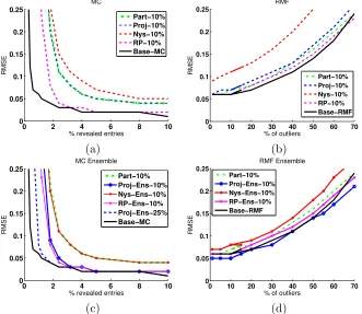
Figure 1: Recovery error of DFCrelative to base algorithms.
We first explored the estimation error of DFC as a function of s, using (m = 10K, r = 10) with varying observation sparsity for MC and (m = 1K, r = 10) with a varying percentage of outliers for RMF. The results are summarized in Figure 1. In both MC and RMF, the gaps in estimation between APG and DFCare small when sampling only 10%
of rows and columns. Moreover, of the standard DFCalgorithms, DFC-RP performs the
best, as shown in Figures 1(a) and (b). Ensembling improves the performance of DFC-Nysand DFC-Proj, as shown in Figures 1(c) and (d), andDFC-Proj-Ensin particular
consistently outperforms Partition and DFC-Nys-Ens, slightly outperforms DFC-RP,
of [ ˆC1, . . . ,Cˆt], and thus the performance of DFC-RP consistently matches that of
DFC-RP-Ens. We therefore omit theDFC-RP-Ensresults in the remainder this section.
We next explored the speed-up of DFCas a function of matrix size. For MC, we revealed
4% of the matrix entries and set r = 0.001·m, while for RMF we fixed the percentage of outliers to 10% and setr = 0.01·m. We sampled 10% of rows and columns and observed that estimation errors were comparable to the errors presented in Figure 1 for similar settings of s; in particular, at all values of nfor both MC and RMF, the errors of APG and DFC-Proj-Ens were nearly identical. Our timing results, presented in Figure 2, illustrate a
near-linear speed-up for MC and a superlinear speed-up for RMF across varying matrix sizes. Note that the timing curves of the DFC algorithms and Partition all overlap, a
fact that highlights the minimal computational cost of the final matrix approximation step.
1 2 3 4 5
x 104
0 500 1000 1500 2000 2500 3000 3500
MC
time (s)
m Part−10% RP−10% Proj−Ens−10% Nys−Ens−10% Base−RMF
1000 2000 3000 4000 5000
0 0.5 1 1.5 2
2.5x 10
4 RMF
time (s)
m
Part−10% RP−10% Proj−Ens−10% Nys−Ens−10% Base−RMF
Figure 2: Speed-up of DFCrelative to base algorithms.
6.2 Collaborative Filtering
Collaborative filtering for recommender systems is one prevalent real-world application of noisy matrix completion. A collaborative filtering data set can be interpreted as the in-complete observation of a ratings matrix with columns corresponding to users and rows corresponding to items. The goal is to infer the unobserved entries of this ratings matrix. We evaluate DFCon two of the largest publicly available collaborative filtering data sets:
MovieLens 10M (http://www.grouplens.org/) with m = 10K, n = 72K, s >10M, and the Netflix Prize data set (http://www.netflixprize.com/) with m = 18K, n = 480K,
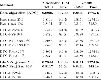
s > 100M. To generate test sets drawn from the training distribution, for each data set, we aggregated all available rating data into a single training set and withheld test entries uniformly at random, while ensuring that at least one training observation remained in each row and column. The algorithms were then run on the remaining training portions and evaluated on the test portions of each split. The results, averaged over three train-test splits, are summarized in Table 2. Notably,DFC-Proj,DFC-Proj-Ens,DFC-Nys-Ens,
and DFC-RP all outperform Partition, and DFC-Proj-Ens performs comparably to
APG while providing a nearly linear parallel time speed-up. Similar to the simulation re-sults presented in Figure 1, DFC-RPperforms the best of the standard DFCalgorithms,
thoughDFC-Proj-Ensslightly outperformsDFC-RP. Moreover, the poorer performance
of DFC-Nys can be in part explained by the asymmetry of these problems. Since these
Method MovieLens 10M Netflix
RMSE Time RMSE Time
Base algorithm (APG) 0.8005 552.3s 0.8433 4775.4s
Partition-25% 0.8146 146.2s 0.8451 1274.6s
Partition-10% 0.8461 56.0s 0.8491 548.0s
DFC-Nys-25% 0.8449 141.9s 0.8832 1541.2s
DFC-Nys-10% 0.8776 82.5s 0.9228 797.4s
DFC-Nys-Ens-25% 0.8085 153.5s 0.8486 1661.2s
DFC-Nys-Ens-10% 0.8328 96.2s 0.8613 909.8s
DFC-Proj-25% 0.8061 146.3s 0.8436 1274.8s
DFC-Proj-10% 0.8270 56.0s 0.8486 548.1s
DFC-Proj-Ens-25% 0.7944 146.3s 0.8411 1274.8s DFC-Proj-Ens-10% 0.8117 56.0s 0.8434 548.1s
DFC-RP-25% 0.8027 147.4s 0.8438 1283.6s
DFC-RP-10% 0.8074 56.2s 0.8448 550.1s
Table 2: Performance of DFC relative to base algorithm APG on collaborative filtering
tasks.
easier than MF on row submatrices, and for DFC-Nys, we observe that ˆC is an accurate
estimate while ˆR is not.
6.3 Background Modeling in Computer Vision
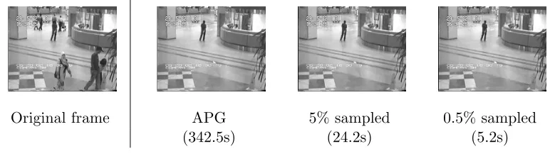
Background modeling has important practical ramifications for detecting activity in surveil-lance video. This problem can be framed as an application of noisy RMF, where each video frame is a column of some matrix (M), the background model is low-rank (L0), and moving objects and background variations, e.g., changes in illumination, are outliers (S0). We evalu-ateDFCon two videos (treating each frame as a row): ‘Hall’ (200 frames of size 176×144)
contains significant foreground variation and was studied by Cand`es et al. (2011), while ‘Lobby’ (1546 frames of size 168×120) includes many changes in illumination (a smaller video with 250 frames was studied by Cand`es et al. 2011). We focused onDFC-Proj-Ens,
due to its superior performance in previous experiments, and measured the RMSE between the background model estimated by DFCand that of APG. On both videos, DFC-Proj-Ens estimated nearly the same background model as the full APG algorithm in a small
fraction of the time. On ‘Hall,’ theDFC-Proj-Ens-5% andDFC-Proj-Ens-0.5% models
Original frame APG 5% sampled 0.5% sampled
(342.5s) (24.2s) (5.2s)
Figure 3: Sample ‘Hall’ estimation by APG, DFC-Proj-Ens-5%, and DFC-Proj-Ens -.5%.
the RMSE of DFC-Proj-Ens-4% was 0.64, and the speed-up over APG was more than
20X, i.e., the running time reduced from 16557s to 792s.
6.4 From Theory to Practice
Our experimental results suggest that the theoretical error bounds of Secs. 4 and 5 can be further tightened. In particular, our master theorems Theorems 12 and 20 guarantee that
DFC-Proj-Ens and DFC-RP are never more than a constant factor worse than
Par-tition, yet in both real data experiments and simulations we observe significant gains in accuracy over Partition due to the incorporation of projection and ensembling.
More-over, our theory gives rise to comparable estimation guarantees forDFC-Nys, albeit under
stronger assumptions as noted in Remark 13. This is a surprising fact given thatDFC-Nys
may make use of only a vanishingly small subset of all available matrix entries; however, we find that for data sets with high noise levels, methods that make use of all available data
likeDFC-ProjandDFC-RP are unsurprisingly more accurate thanDFC-Nys. We view
addressing these gaps between theory and practice as important directions for future work.
7. Conclusions
To improve the scalability of existing matrix factorization algorithms while leveraging the ubiquity of parallel computing architectures, we introduced, evaluated, and analyzedDFC,
a divide-and-conquer framework for noisy matrix factorization with missing entries or out-liers. DFCis trivially parallelized and particularly well suited for distributed environments
given its low communication footprint. Moreover,DFCprovably maintains the estimation
guarantees of its base algorithm, even in the presence of noise, and yields linear to super-linear speedups in practice. A number of natural follow-up questions suggest themselves:
• How does DFC compare empirically with scalable heuristics for MC and RMF that
have little theoretical backing (see, e.g., Zhou et al., 2008; Gemulla et al., 2011; Recht and R´e, 2011; F. Niu et al., 2011; Yu et al., 2012; Mu et al., 2011)? Is improved perfor-mance obtained by pairing DFCwith base algorithms lacking theoretical guarantees
but displaying other practical benefits?
• Which algorithmic refinements lead to enhanced performance forDFC? For instance,
could ensemble variants of DFC be improved by learning combination weights in a
manner analogous to that of Kumar et al. (2009b)? In the matrix completion setting, could one use held-out entries to determine the optimal dimension (via rows or via columns) for partitioning inDFC-ProjorDFC-RP?
These open questions are fertile ground for future work.
Acknowledgments
Lester Mackey gratefully acknowledges the support of DARPA through the National De-fense Science and Engineering Graduate Fellowship Program. Ameet Talwalkar gratefully acknowledges support from NSF award No. 1122732.
Appendix A. Proof of Theorem 5: Subsampled Regression under Incoherence
We now give a proof of Theorem 5. While the results of this section are stated in terms of i.i.d. with-replacement sampling of columns and rows, a concise argument due to Hoeffding (1963, Section 6) implies the same conclusions when columns and rows are sampled without replacement.
Our proof of Theorem 5 will require a strengthened version of the randomized`2 regres-sion work of Drineas et al. (2008, Theorem 5). The proof of Theorem 5 of Drineas et al. (2008) relies heavily on the fact that kAB−GHkF ≤
2kAkFkBkF with probability at least 0.9, when G and H contain sufficiently many rescaled columns and rows of A and B, sampled according to a particular non-uniform probability distribution. A result of Hsu et al. (2012), modified to allow for slack in the probabilities, establishes a related claim with improved sampling complexity.6
Lemma 24 (Hsu et al. 2012, Example 4.3) Given a matrixA∈Rm×kwithr≥rank(A),
an error tolerance ∈ (0,1], and a failure probability δ ∈(0,1], define probabilities pj
sat-isfying
pj ≥
β
ZkA(j)k
2
, Z =X
j
kA(j)k2, and
Pk
j=1pj = 1
for some β ∈ (0,1]. Let G ∈ Rm×l be a column submatrix of A in which exactly l ≥ 48rlog(4r/(βδ))/(β2)columns are selected in i.i.d. trials in which thej-th column is chosen with probability pj. Further, let D ∈Rl×l be a diagonal rescaling matrix with entry Dtt = 1/p
lpj whenever thej-th column ofAis selected on thet-th sampling trial, for t= 1, . . . , l.
Then, with probability at least 1−δ,
kAA>−GDDG>k2≤ 2kAk
2 2.
Using Lemma 24, we now establish a stronger version of Lemma 1 of Drineas et al. (2008). For a given β ∈(0,1] and L∈Rm×n with rank r, we first define column sampling probabilities pj satisfying
pj ≥
β
rk(VL)(j)k
2 and Pn
j=1pj = 1. (4)
We further let S ∈ Rn×l be a random binary matrix with independent columns, where a single 1 appears in each column, and Sjt = 1 with probability pj for each t ∈ {1, . . . , l}. Moreover, let D∈Rl×l be a diagonal rescaling matrix with entry Dtt = 1/plpj whenever Sjt = 1. Postmultiplication by S is equivalent to selectingl random columns of a matrix, independently and with replacement. Under this notation, we establish the following lemma:
Lemma 25 Let ∈ (0,1], and define V>l = V>LS and Γ = (V>l D)+ −(V> l D)
>. If
l≥48rlog(4r/(βδ))/(β2) for δ∈(0,1] then with probability at least1−δ: rank(Vl) = rank(VL) = rank(L)
kΓk2 =kΣ−1V>
l D
−ΣV>
l Dk2 (LSD)+= (V>l D)+Σ−1L U>L
kΣ−1V>
l D
−ΣV>
l Dk2≤/ √
2.
Proof By Lemma 24, for all 1≤i≤r,
|1−σ2i(V>l D)|=|σi(V>LVL)−σi(Vl>DDVl)| ≤ kVL>VL−V>LSDDS>VLk2 ≤/2kVL>k22 =/2,
whereσi(·) is thei-th largest singular value of a given matrix. Since/2≤1/2, each singu-lar value of Vl is positive, and so rank(Vl) = rank(VL) = rank(L). The remainder of the proof is identical to that of Lemma 1 of Drineas et al. (2008).
Lemma 25 immediately yields improved sampling complexity for the randomized `2 regression of Drineas et al. (2008):
Proposition 26 Suppose B ∈ Rp×n and ∈ (0,1]. If l ≥ 3200rlog(4r/(βδ))/(β2) for
δ∈(0,1], then with probability at least 1−δ−0.2:
Proof The proof is identical to that of Theorem 5 of Drineas et al. (2008) once Lemma 25 is substituted for Lemma 1 of Drineas et al. (2008).
A typical application of Prop. 26 would involve performing a truncated SVD of M to obtain the statistical leverage scores, k(VL)(j)k2, used to compute the column sampling probabilities of Eq. (4). Here, we will take advantage of the slack term, β, allowed in the sampling probabilities of Eq. (4) to show that uniform column sampling gives rise to the same estimation guarantees for column projection approximations when L is sufficiently incoherent.
To prove Theorem 5, we first notice thatn≥rµ0(VL) and hence
l≥3200rµ0(VL) log(4rµ0(VL)/δ)/2 ≥3200rlog(4r/(βδ))/(β2)
whenever β ≥ 1/µ0(VL). Thus, we may apply Prop. 26 with β = 1/µ0(VL) ∈ (0,1] and
pj = 1/nby noting that
β
rk(VL)(j)k
2≤ β
r r
nµ0(VL) =
1
n =pj
for allj, by the definition ofµ0(VL). By our choice of probabilities,D=I
p
n/l, and hence
kB−BCL+CLkF =kB−BCD(LCD)+LkF ≤(1 +)kB−BL+LkF with probability at least 1−δ−0.2, as desired.
Appendix B. Proof of Lemma 4: Conservation of Incoherence
Since for alln >1,
clog(n) log(1/δ) = (c/4) log(n4) log(1/δ)≥48 log(4n2/δ)≥48 log(4rµ0(VL)/(δ/n)) asn≥rµ0(VL), claimifollows immediately from Lemma 25 withβ = 1/µ0(VL),pj = 1/n for all j, and D =Ipn/l. When rank(LC) = rank(L), Lemma 1 of Mohri and Talwalkar (2011) implies that PULC =PUL, which in turn implies claim ii.
To prove claimiiigiven the conclusions of Lemma 25, assume, without loss of generality, that Vl consists of the first l rows of VL. Then if LC = ULΣLV>l has rank(LC) = rank(L) =r, the matrixVl must have full column rank. Thus we can write
L+CLC = (ULΣLV>l )+ULΣLV>l = (ΣLV>l )+U
+
where the second and third equalities follow from UL having orthonormal columns, the fourth and fifth result from ΣL having full rank and Vl having full column rank, and the sixth follows fromV>l having full row rank.
Now, denote the right singular vectors of LC by VLC ∈ Rl×r. Observe that PVLC = VLCV
> LC =L
+
CLC, and defineei,l as theith column of Il and ei,n as theith column of In. Then we have,
µ0(VLC) =
l
r1≤i≤lmaxkPVLCei,lk 2
= l
r1≤i≤lmaxe >
i,lL+CLCei,l = l
r1≤i≤lmaxe > i,l(V
> l )+V
> l ei,l
= l
r1≤i≤lmaxe > i,lVl(V
> l Vl)
−1 Vl>ei,l = l
r1≤i≤lmaxe > i,nVL(V
>
l Vl)−1V>Lei,n,
where the final equality follows from V>l ei,l=VL>ei,n for all 1≤i≤l. Now, defining Q=V>l Vl we have
µ0(VLC) =
l
r1≤i≤lmax e > i,nVLQ
−1
VL>ei,n = l
r1≤i≤lmax Tr
h
e>i,nVLQ−1V>Lei,n
i
= l
r1≤i≤lmax Tr
h
Q−1VL>ei,ne>i,nVL
i
≤ l
rkQ
−1k
21≤i≤lmaxkV >
Lei,ne>i,nVLk∗ ,
by H¨older’s inequality for Schatten p-norms. Since VL>ei,ne>i,nVL has rank one, we can explicitly compute its trace norm as kVL>ei,nk
2
=kPVLei,nk
2. Hence,
µ0(VLC)≤
l rkQ
−1k
21≤i≤lmaxkPVLei,nk 2
≤ l
r r nkQ
−1k 2
n
r 1≤i≤nmax kPVLei,nk 2
= l
nkQ
−1k
2µ0(VL),
To prove claim iv under Lemma 25, we note that
µ1(LC) =
r ml
r 1≤i≤mmax 1≤j≤l
|e>i,mULCV > LCej,l|
≤
r ml
r 1≤i≤mmax kU >
LCei,mk1≤j≤lmax kV > LCej,lk
=√r r
m
r 1≤i≤mmax kPULCei,mk
r l
r1≤j≤lmax kPVLCej,lk
=
q
rµ0(ULC)µ0(VLC)≤
p
rµ0(UL)µ0(VL)/(1−/2)
by H¨older’s inequality for Schatten p-norms, the definition of µ0-coherence, and claims ii and iii.
Appendix C. Proof of Corollary 6: Column Projection under Incoherence
Fixc= 48000/log(1/0.45), and notice that forn >1,
48000 log(n)≥3200 log(n5)≥3200 log(16n).
Hence l≥3200rµ0(VL) log(16n)(log(δ)/log(0.45))/2.
Now partition the columns ofCintob= log(δ)/log(0.45) submatrices,C= [C1,· · · ,Cb], each with a =l/b columns,7 and let [LC1,· · ·,LCb] be the corresponding partition of LC. Since
a≥3200rµ0(VL) log(4n/0.25)/2, we may apply Prop. 26 independently for eachito yield
kM−CiL+CiLkF ≤(1 +)kM−ML+LkF ≤(1 +)kM−LkF (5) with probability at least 0.55, sinceML+ minimizeskM−YLkF over all Y∈Rm×m.
Since each Ci = CSi for some matrix Si and C+M minimizes kM−CXkF over all X∈Rl×n, it follows that
kM−CC+MkF ≤ kM−CiL+C iLkF,
for each i. Hence, if
kM−CC+MkF ≤(1 +)kM−LkF,
fails to hold, then, for each i, Eq. (5) also fails to hold. The desired conclusion therefore must hold with probability at least 1−0.45b = 1−δ.
Appendix D. Proof of Corollary 7: Generalized Nystr¨om Method under Incoherence
Withc= 48000/log(1/0.45) as in Corollary 6, we notice that form >1,
48000 log(m) = 16000 log(m3)≥16000 log(4m).
Therefore,
d≥16000rµ0(UC) log(4m)(log(δ0)/log(0.45))/2 ≥3200rµ0(UC) log(4m/δ0)/2,
for all m > 1 and δ0 ≤0.8. Hence, we may apply Theorem 5 and Corollary 6 in turn to obtain
kM−CW+RkF ≤(1 +)kM−CC+MkF ≤(1 +)2kM−Lk with probability at least (1−δ)(1−δ0−0.2) by independence.
Appendix E. Proof of Corollary 8: Noiseless Generalized Nystr¨om Method under Incoherence
Since rank(L) = r, L admits a decomposition L = Y>Z for some matrices Y ∈ Rr×m and Z ∈ Rr×n. In particular, let Y> = ULΣ
1 2
L and Z = Σ 1 2 LV
>
L. By block partitioning Y and Z as Y =
Y1 Y2
and Z =
Z1 Z2
for Y1 ∈ Rr×d and Z1 ∈ Rr×l, we may write W =Y1>Z1,C=Y>Z1, and R=Y1>Z. Note that we assume that the generalized Nystr¨om approximation is generated from sampling the firstl columns and the firstdrows of L, which we do without loss of generality since the rows and columns of the original low-rank matrix can always be permuted to match this assumption.
Prop. 27 shows that, like the Nystr¨om method (Kumar et al., 2009a), the generalized Nystr¨om method yields exact recovery ofLwhenever rank(L) = rank(W). The same result was established in Wang et al. (2009) with a different proof.
Proposition 27 Suppose r= rank(L)≤min(d, l) and rank(W) =r. Then L=Lnys.
Proof By appealing to our factorized block decomposition, we may rewrite the generalized Nystr¨om approximation as Lnys = CW+R = Y>Z1(Y1>Z1)+Y1>Z. We first note that rank(W) = r implies that rank(Y1) = r and rank(Z1) = r so that Z1Z>1 and Y1Y>1 are full-rank. Hence, (Y>1Z1)+=Z>1(Z1Z>1)−1(Y1Y>1)−1Y1,yielding
Lnys=Y>Z1Z>1(Z1Z>1)−1(Y1Y>1)−1Y1Y>1Z=Y>Z=L.