On the properties of variational approximations of Gibbs
posteriors
Pierre Alquier pierre.alquier@ensae.fr
James Ridgway james.ridgway@ensae.fr
Nicolas Chopin nicolas.chopin@ensae.fr
ENSAE
3 Avenue Pierre Larousse 92245 MALAKOFF, FRANCE
Editor: Yee Whye Teh
Abstract
The PAC-Bayesian approach is a powerful set of techniques to derive non-asymptotic risk bounds for random estimators. The corresponding optimal distribution of estimators, usually called the Gibbs posterior, is unfortunately often intractable. One may sample from it using Markov chain Monte Carlo, but this is usually too slow for big datasets. We consider instead variational approximations of the Gibbs posterior, which are fast to compute. We undertake a general study of the properties of such approximations. Our main finding is that such a variational approximation has often the same rate of convergence as the original PAC-Bayesian procedure it approximates. In addition, we show that, when the risk function is convex, a variational approximation can be obtained in polynomial time using a convex solver. We give finite sample oracle inequalities for the corresponding estimator. We specialize our results to several learning tasks (classification, ranking, matrix completion), discuss how to implement a variational approximation in each case, and illustrate the good properties of said approximation on real datasets.
1. Introduction
A Gibbs posterior, also known as a PAC-Bayesian or pseudo-posterior, is a probability distribution for random estimators of the form:
ˆ
ρλ(dθ) = Rexp[−λrn(θ)] exp[−λrn]dπ
π(dθ).
More precise definitions will follow, but for now,θmay be interpreted as a parameter (in a finite or infinite-dimensional space),rn(θ) as an empirical measure of risk (e.g. prediction error), and π(dθ) a prior distribution.
McAllester, 1998; Catoni, 2004); see Catoni (2007) for an exhaustive study, and Jiang and Tanner (2008); Yang (2004); Zhang (2006); Dalalyan and Tsybakov (2008) for related per-spectives (such as the aggregation of estimators in the last three papers). There, ˆρλ appears as the probability distribution that minimizes the upper bound of an oracle inequality on the risk of random estimators. The PAC-Bayesian approach offers sharp theoretical guar-antees on the properties of such estimators, without assuming a particular model for the data generating process.
The Gibbs posterior has also appeared in other places, and under different motivations: in Econometrics, as a way to avoid direct maximization in moment estimation (Cher-nozhukov and Hong, 2003); and in Bayesian decision theory, as a way to define a Bayesian posterior distribution when no likelihood has been specified (Bissiri et al., 2013). Another well-known connection, although less directly useful (for Statistics), is with thermodynam-ics, where rn is interpreted as an energy function, andλas the inverse of a temperature.
Whatever the perspective, estimators derived from Gibbs posteriors usually show excel-lent performance in diverse tasks, such as classification, regression, ranking, and so on, yet their actual implementation is still far from routine. The usual recommendation (Dalalyan and Tsybakov, 2012; Alquier and Biau, 2013; Guedj and Alquier, 2013) is to sample from a Gibbs posterior using MCMC (Markov chain Monte Carlo, see e.g. Green et al., 2015); but constructing an efficient MCMC sampler is often difficult, and even efficient implemen-tations are often too slow for practical uses when the dataset is very large.
In this paper, we consider instead VB (Variational Bayes) approximations, which have been initially developed to provide fast approximations of ‘true’ posterior distributions (i.e. Bayesian posterior distributions for a given model); see Jordan et al. (1999); MacKay (2002) and Chap. 10 in Bishop (2006).
Our main results are as follows: when PAC-Bayes bounds are available - mainly, when a strong concentration inequality holds - replacing the Gibbs posterior by a variational approximation does not affect the rate of convergence to the best possible prediction, on the condition that the K¨ullback-Leibler divergence between the posterior and the approx-imation is itself properly controlled. Furthermore, for convex risks we show that one can obtain polynomial time algorithms based on optimal convex solvers.
We also provide empirical bounds, which may be computed from the data to ascertain the actual performance of estimators obtained by variational approximation. All the re-sults gives strong incentives, we believe, to recommend Variational Bayes as the default approach to approximate Gibbs posteriors. We also provide a R package1, written in C++ to compute a Gaussian variational approximation in the case of the hinge risk.
The rest of the paper is organized as follows. In Section 2, we present the notations and assumptions. In Section 3, we introduce variational approximations and the corresponding algorithms. The main results are provided in a general form in Section 4: in Subsection 4.1, we give results under the assumption that a Hoeffding type inequality holds (slow rates) and
in Subsection 4.2, we give results under the assumption that a Bernstein type inequality holds (fast rates). Note that for the sake of brevity, we will refer to these settings as “Hoeffding assumption” and “Bernstein assumption” even though this terminology is non-standard. We then apply these results in various settings: classification (Section 5), convex classification (Section 6), ranking (Section 7), and matrix completion (Section 8). In each case, we show how to specialise the general results of Section 4 to the considered application, in order to obtain the properties of the VB approximation, and we also discuss its numerical implementation. All the proofs are collected in the Appendix.
2. PAC-Bayesian framework
We observe a sample (X1, Y1), . . . ,(Xn, Yn), taking values inX ×Y, where the pairs (Xi, Yi) have the same distributionP. We will assume explicitly that the (Xi, Yi)’s are independent in several of our specialised results, but we do not make this assumption at this stage, as some of our general results, and more generally the PAC-Bayesian theory, may be extended to dependent observations; see e.g. Alquier and Li (2012). The label setYis always a subset of R. A set of predictors is chosen by the statistician: {fθ :X →R, θ∈Θ}.For example,
in linear regression, we may have: fθ(x) = hθ, xi, the inner product of X = Rd, while in
classification, one may have fθ(x) =Ihθ,xi>0∈ {0,1}.
We assume we have at our disposal a risk function R(θ); typically R(θ) is a measure of the prediction error. We set R = R(θ), where θ ∈ arg minΘR; i.e. fθ is an optimal predictor. We also assume that the risk functionR(θ) has an empirical counterpart rn(θ), and set rn = rn(θ). Often, R and rn are based on a loss function ` : R2 → R; i.e.
R(θ) = E[`(Y, fθ(X))] and rn(θ) = 1n Pn
i=1`(Yi, fθ(Xi)). (In this paper, the symbol E will always denote the expectation with respect to the (unknown) lawP of the (Xi, Yi)’s.) There are situations however (e.g. ranking), whereR and rnhave a different form.
We define a prior probability measure π(·) on the set Θ (equipped with the standard
σ-algebra for the considered context), and we letM1
+(Θ) denote the set of all probability measures on Θ.
Definition 2.1 We define, for any λ >0, the pseudo-posteriorρˆλ by
ˆ
ρλ(dθ) =
exp[−λrn(θ)] R
exp[−λrn]dπ
π(dθ).
certain model, ˆρλ becomes a Bayesian posterior distribution, but we will not restrict our attention to this particular case.
The following ‘theoretical’ counterpart of ˆρλ will prove useful to state results.
Definition 2.2 We define, for any λ >0, πλ as
πλ(dθ) =
exp[−λR(θ)] R
exp[−λR]dππ(dθ).
We will derive PAC-Bayesian bounds on predictions obtained by variational approxima-tions of ˆρλ under two types of assumptions: a Hoeffding-type assumption, from which we may deduce slow rates of convergence (Subsection 4.1), and a Bernstein-type assumption, from which we may obtain fast rates of convergence (Subsection 4.2).
Definition 2.3 We say that a Hoeffding assumption is satisfied for prior π when there is a function f and an interval I ⊂R∗+ such that, for any λ∈I, for anyθ∈Θ,
π(Eexp{λ[R(θ)−rn(θ)]})
π(Eexp{λ[rn(θ)−R(θ)]})
≤exp [f(λ, n)]. (1)
Inequality (1) can be interpreted as an integrated version (with respect to π) of Ho-effding’s inequality, for which f(λ, n) λ2/n. In many cases the loss will be bounded uniformly overθ; then Hoeffding’s inequality will directly imply (1). The expectation with respect to π in (1) allows us to treat some cases where the loss is not upper bounded by specifying a prior with sufficiently light tails.
Definition 2.4 We say that a Bernstein assumption is satisfied for prior π when there is a function g and an interval I ⊂R∗+ such that, for any λ∈I, for anyθ∈Θ,
π Eexpλ[R(θ)−R]−λ[rn(θ)−rn]
π Eexpλ[rn(θ)−rn]−λ[R(θ)−R]
≤π exp
g(λ, n)[R(θ)−R]
. (2)
This assumption is satisfied for example by sums of i.i.d. sub-exponential random variables, see Subsection 2.4 p. 27 in Boucheron et al. (2013), when a margin assumption on the functionR(·) is satisfied (Tsybakov, 2004). This is discussed in Section 4.2. Again, extensions beyond the i.i.d. case are possible, see e.g. Wintenberger (2010) for a survey and new results. In all these examples, the important feature of the function g that we will use to derive rates of convergence is the fact that there is a constant c >0 such that when λ=cn,g(λ, n) =g(cn, n)n.
As mentioned previously, we will often considerrn(θ) = n1Pn
Remark 2.1 We could consider more generally inequalities of the form
π Eexpλ[R(θ)−R]−λ[rn(θ)−rn]
π Eexpλ[rn(θ)−rn]−λ[R(θ)−R]
≤π exp
g(λ, n)[R(θ)−R]κ
that allow using the more general form of the margin assumption of Mammen and Tsybakov (1999); Tsybakov (2004). PAC-Bayes bounds in this context are provided by Catoni (2007). However, the techniques involved would require many pages to be described so we decided to focus on the cases κ= 0 and κ= 1 to keep the exposition simple.
3. Numerical approximations of the pseudo-posterior
3.1 Monte Carlo
As already explained in the introduction, the usual approach to approximate ˆρλ is MCMC (Markov chain Monte Carlo) sampling. Ridgway et al. (2014) proposed tempering SMC (Sequential Monte Carlo, e.g. Del Moral et al. (2006)) as an alternative to MCMC to sample from Gibbs posteriors: one samples sequentially from ˆρλt, with 0 = λ0 < · · · < λT = λ
where λ is the desired temperature. One advantage of this approach is that it makes it possible to contemplate different values of λ, and choose one by e.g. cross-validation. Another advantage is that such an algorithm requires little tuning; see Appendix B for more details on the implementation of tempering SMC. We will use tempering SMC as our gold standard in our numerical studies.
SMC and related Monte Carlo algorithms tend to be too slow for practical use in situations where the sample size is large, the dimension of Θ is large, orfθ is expensive to compute. This motivates the use of fast, deterministic approximations, such as Variational Bayes, which we describe in the next section.
3.2 Variational Bayes
Various versions of VB (Variational Bayes) have appeared in the literature, but the main idea is as follows. We define a family F ⊂ M1
+(Θ) of probability distributions that are considered as tractable. Then, we define the VB-approximation of ˆρλ: ˜ρλ.
Definition 3.1 Let
˜
ρλ= arg min
ρ∈FK(ρ,ρˆλ),
where K(ρ,ρˆλ)denotes the KL (K¨ullback-Leibler) divergence of ρˆλ relative toρ: K(m, µ) = R
log[dmdµ]dm if mµ (i.e. µ dominates m),K(m, µ) = +∞ otherwise.
The difficulty is to find a familyF (a) which is large enough, so that ˜ρλ may be close to ˆ
or less strong guarantees on the quality of the optimization. For example, while in Section 6 we consider a setting where an exact upper bound for the optimization error is available, in Section 8 this is no longer the case.
We now review two types of families popular in the VB literature.
• Mean field VB: for a certain decomposition Θ = Θ1×. . .×Θd,F is the set of product probability measures
FMF= (
ρ∈ M1+(Θ) :ρ(dθ) = d Y
i=1
ρi(dθi),∀i∈ {1, . . . , d}, ρi ∈ M1+(Θi) )
. (3)
The infimum of the KL divergenceK(ρ,ρˆλ), relative toρ= Q
iρi satisfies the follow-ing fixed point condition (Parisi, 1988; Bishop, 2006, Chap. 10):
∀j ∈ {1,· · ·, d} ρj(dθj)∝exp
Z
{−λrn(θ) + logπ(θ)} Y
i6=j
ρi(dθi)
π(dθj). (4)
This leads to a natural algorithm were we update successively every ρj until stabi-lization.
• Parametric family:
FP=
ρ∈ M1+(Θ) :ρ(dθ) =f(θ;m)dθ, m∈M ;
and M is finite-dimensional; say FP is the family of Gaussian distributions (of di-mension d). In this case, several methods may be used to compute the infimum. As above, one may used fixed-point iteration, provided an equation similar to (4) is available. Alternatively, one may directly maximizeR log[exp[−λrn(θ)]dπdρ(θ)]ρ(dθ) with respect to parameter m, using numerical optimization routines. This approach was used for instance in Hoffman et al. (2013) with combination of some stochastic gradient descent to perform inference on a latent Dirichlet allocation model. See also e.g. Khan (2014); Khan et al. (2013) for efficient algorithms for Gaussian variational approximation.
In what follows (Subsections 4.1 and 4.2) we provide tight bounds for the prediction risk of ˜ρλ. This leads to the identification of a condition on F such that the risk of ˜ρλ is not worse than the risk of ˆρλ. We will make this condition explicit in various examples, using either mean field VB or parametric approximations.
Remark 3.1 An useful identity, obtained by direct calculations, is: for any ρπ,
log Z
exp [−λrn(θ)]π(dθ) =−λ
Z
Since the left hand side does not depend on ρ, one sees that ρ˜λ, which minimizes K(ρ,ρˆλ)
over F, is also the minimizer of:
˜
ρλ = arg min ρ∈F
Z
rn(θ)ρ(dθ) + 1
λK(ρ, π)
This equation will appear frequently in the sequel in the form of an empirical upper bound.
4. General results
This section gives our general results, under either a Hoeffding Assumption (Definition 2.3) or a Bernstein Assumption (Definition 2.4), on risks bounds for the variational ap-proximation, and how it relates to risks bounds for Gibbs posteriors. These results will be specialised to several learning problems in the following sections.
4.1 Bounds under the Hoeffding assumption
4.1.1 Empirical bounds
Theorem 4.1 Under the Hoeffding assumption (Definition 2.3), for any ε >0, with prob-ability at least 1−εwe have simultaneously for any ρ∈ M1
+(Θ), Z
Rdρ≤ Z
rndρ+f(λ, n) +K(ρ, π) + log 1 ε
λ .
This result is a simple variant of a result in Catoni (2007) but for the sake of complete-ness, its proof is given in Appendix A. It gives us an upper bound on the risk of both the pseudo-posterior (takeρ= ˆρλ) and its variational approximation (take ρ= ˜ρλ). These bounds may be be computed from the data, and therefore provide a simple way to evaluate the performance of the corresponding procedure, in the spirit of the first PAC-Bayesian inequalities (Shawe-Taylor and Williamson, 1997; McAllester, 1998, 1999). However, these bounds do not provide the rate of convergence of these estimators. For this reason, we also provide oracle-type inequalities.
4.1.2 Oracle-type inequalities
Another way to use PAC-Bayesian bounds is to compare RRd ˆρλ to the best possible risk, thus linking this approach to oracle inequalities. This is the point of view developed in Catoni (2004, 2007); Dalalyan and Tsybakov (2008).
Theorem 4.2 Assume that the Hoeffding assumption is satisfied (Definition 2.3). For any ε >0, with probability at least 1−ε we have simultaneously
Z
Rd ˆρλ ≤ Bλ(M1+(Θ)) := inf ρ∈M1
+(Θ)
( Z
Rdρ+ 2f(λ, n) +K(ρ, π) + log 2 ε
λ
and
Z
Rd ˜ρλ≤ Bλ(F) := inf ρ∈F
( Z
Rdρ+ 2f(λ, n) +K(ρ, π) + log 2 ε
λ
)
.
Moreover,
Bλ(F) =Bλ(M1+(Θ)) + 2
λρinf∈FK(ρ, πλ2) where we remind that πλ is defined in Definition 2.2.
In this way, we are able to compareR
Rd ˆρλ to the best possible aggregation procedure inM1
+(Θ) and R
Rd ˜ρλ to the best aggregation procedure inF. More importantly, we are able to obtain explicit expressions for the right-hand side of these inequalities in various models, and thus to obtain rates of convergence. This will be done in the remaining sections. This leads to the second interest of this result: if there is a λ=λ(n) that leads to Bλ(M1
+(Θ)) ≤R+sn with sn → 0 for the pseudo-posterior ˆρλ, then we only have to prove that there is a ρ∈ F such that K(ρ, πλ)/λ≤csn for some constant c >0 to ensure that the VB approximation ˜ρλ also reaches the rate sn.
We will see in the following sections several examples where the approximation does not deteriorate the rate of convergence. But first let us show the equivalent oracle inequality under the Bernstein assumption.
4.2 Bounds under the Bernstein assumption
In this context the empirical bound on the risk would depend on the minimal achievable risk ¯rn, and cannot be computed explicitly. We give the oracle inequality for both the Gibbs posterior and its VB approximation in the following theorem.
Theorem 4.3 Assume that the Bernstein assumption is satisfied (Definition 2.4). Assume that λ∈I satisfies λ−g(λ, n)>0. Then for anyε >0, with probability at least1−εwe have simultaneously:
Z
Rd ˆρλ−R≤ Bλ M1+(Θ)
,
Z
Rd ˜ρλ−R≤ Bλ(F),
where, for either A=M1
+(Θ) or A=F, Bλ(A) = 1
λ−g(λ, n)ρinf∈A
(
[λ+g(λ, n)] Z
(R−R)dρ+ 2K(ρ, π) + 2 log
2
ε
)
.
In addition,
Bλ(F) =Bλ M1+(Θ)
+ 2
λ−g(λ, n)ρinf∈FK
ρ, πλ+g(λ,n) 2
The main difference with Theorem 4.2 is that the functionR(·) is replaced byR(·)−R. This is well known way to obtain better rates of convergence.
5. Application to classification
5.1 Preliminaries
In all this section, we assume that Y ={0,1} and we consider linear classification: Θ = X =Rd,fθ(x) =1hθ,xi≥0. We putrn(θ) = n1Pni=11{fθ(Xi)6=Yi},R(θ) =P(Y 6=fθ(X)) and
assume that the [(Xi, Yi)]ni=1 are i.i.d. In this setting, it is well-known that the Hoeffding assumption always holds. We state as a reminder the following lemma.
Lemma 1 Hoeffding assumption (1) is satisfied withf(λ, n) =λ2/(2n), λ∈R+.
The proof is given in Appendix A for the sake of completeness.
It is also possible to prove that Bernstein assumption (2) holds in the case where the so-called margin assumption of Mammen and Tsybakov is satisfied. This condition we use was introduced by Tsybakov (2004) in a classification setting, based on a related definition in Mammen and Tsybakov (1999).
Lemma 2 Assume that Mammen and Tsybakov’s margin assumption is satisfied: i.e. there is a constant C such that
E[(1fθ(X)6=Y −1fθ(X)6=Y)
2]≤C[R(θ)−R].
Then Bernstein assumption (2) is satisfied withg(λ, n) = 2nCλ−2λ.
Remark 5.1 We refer the reader to Tsybakov (2004) for a proof that
P(0<|θ, X|≤t)≤C0t
for some constant C0 >0 implies the margin assumption. In words, when X is not likely to be in the region
θ, X
'0, where points are hard to classify, then the problem becomes easier and the classification rate can be improved.
5.2 Three sets of Variational Gaussian approximations
Consider the three following Gaussian families
F1=nΦm,σ2,m∈Rd, σ2∈R∗+
o
,
F2= n
Φm,σ2,m∈Rd,σ2 ∈(R∗+)d
o
(mean field approximation),
F3=nΦm,Σ,m∈Rd,Σ∈ Sd+
o
(full covariance approximation),
where Φm,σ2 is Gaussian distributionNd(m, σ2Id), Φm,σ2 isNd(m,diag(σ2)), and Φm,Σ is
Nd(m,Σ). Obviously,F1⊂ F2⊂ F3 ⊂ M1+(Θ), and Bλ(M1
+(Θ))≤ Bλ(F3)≤ Bλ(F2)≤ Bλ(F1). (6) Note that, for the sake of simplicity, we will use the following classical notations in the rest of the paper: ϕ(·) is the density ofN(0,1) w.r.t. the Lebesgue measure, and Φ(·) the corresponding c.d.f. The rest of Section 5 is organized as follows. In Subsection 5.3, we calculate explicitly Bλ(F2) and Bλ(F1). Thanks to (6) this also gives an upper bound on Bλ(F3) and proves the validity of the three types of Gaussian approximations. Then, we give details on algorithms to compute the variational approximation based onF2 andF3, and provide a numerical illustration on real data.
5.3 Theoretical analysis
We start with the empirical bound for F2 (and F1 as a consequence), which is a direct corollary of Theorem 4.1.
Corollary 5.1 For any ε > 0, with probability at least 1−ε we have, for any m ∈ Rd,
σ2 ∈(R+)d, Z
RdΦm,σ2 ≤
Z
rndΦm,σ2 +
λ
2n+
1 2
Pd i=1
h logϑσ22
i
+σ2i
ϑ2
i
+k2ϑmk22 − d2 + log 1ε
λ .
We now want to apply Theorem 4.2 in this context. In order to do so, we introduce an additional assumption.
Definition 5.1 We say that Assumption A1 is satisfied when there is a constant c > 0
such that, for any (θ, θ0)∈Θ2 withkθk=kθ0k= 1, P(hX, θi hX, θ0i<0)≤ckθ−θ0k.
This is not a strong assumption. It is satisfied when X has an isotropic distribution, and more generally when X/kXk has a bounded density on the unit sphere2. The intuition
2. If the density ofX/kXkwith respect to the uniform measure on the unit sphere is upper bounded by
BthenP(hX, θi hX, θ0i<0)≤ 2Bπarccos(hθ, θ 0i
)≤ B
2π p
5−5hθ, θ0i ≤ B
2π q
5 2kθ−θ
0k
beyond A1 is that for a “typical” X, a very small change in θ will only induce a change in sign(hX, θi) with a small probability. When it is not satisfied, two parameters θ and
θ0 very close to each other can lead to very different predictions, and thus, whatever the accuracy of an approximation of ¯θ, it might still lead to poor predictions.
Corollary 5.2 Assume that the VB approximation is done on either F1, F2 or F3. Take
λ=√nd andϑ= √1
d. Under Assumption A1, for anyε >0, with probability at least1−ε
we have simultaneously
R
Rd ˆρλ R
Rd ˜ρλ
≤R+ r
d
nlog (4ne) + c
√
n+
1 4n
r
d n+
2 log 2ε √
nd .
See the appendix for a proof. Note also that the values λ = √nd and ϑ = √1
d allow to derive this almost optimal rate of convergence, but are not necessarily the best choices in practice.
Remark 5.2 Note that Assumption A1 is not necessary to obtain oracle inequalities on the risk integrated under ρˆλ. We refer the reader to Chapter 1 in Catoni (2007) for such
assumption-free bounds. However, it is clear that without this assumption the shape of ρˆλ
and ρ˜λ might be very different. Thus, it seems reasonable to require that A1 is satisfied for
the approximation of ρˆλ by ρ˜λ to make sense.
We finally provide an application of Theorem 4.3. Under the additional constraint that the margin assumption is satisfied, we obtain a better rate.
Corollary 5.3 Assume that the VB approximation is done on either F1, F2 or F3. Un-der Assumption A1 (Definition 5.1 page 10), and unUn-der Mammen and Tsybakov margin assumption, with λ= C+22n and ϑ >0, for any ε >0, with probability at least 1−ε,
R
Rd ˆρλ R
Rd ˜ρλ
≤R¯+(C+ 2)(C+ 1) 2
dlogn ϑ
n +
dϑ n2 +
1
ϑ− d ϑn +
2
nlog
2
ε
+
√
d2c(2C+ 1)
n .
It is possible to minimze the bound with respect to ϑ explicitely, this choice or any constant instead will lead to a rate in dlog(n)/n. Note that the rate d/n is minimax-optimal in this context. This is, for example, a consequence of more general results in Lecu´e (2007) under a general form of the the margin assumption. See the Appendix for a proof.
5.4 Implementation and numerical results
For family F2 (mean field), the variational lower bound (5) equals
Lλ,ϑ(m,σ) =−λ
n
n X
i=1
Φ −Yi
Xim p
Xidiag(σ2)Xt i
! −m
Tm 2ϑ +
1 2
d X
k=1
logσ2k−σ 2 k
ϑ
while for family F3 (full covariance), it equals
Lλ,ϑ(m,Σ) =−λ
n
n X
i=1
Φ −Yi
Xim p
XiΣXit
! −m
Tm 2ϑ +
1 2
log|Σ|−1
ϑtrΣ
.
Both functions are non-convex, but the multimodality of the latter may be more se-vere due to the larger dimension of F3. To address this issue, we recommend using the reparametrization of Opper and Archambeau (2009), which makes the dimension of the latter optimization problem O(n); see Khan (2014) for a related approach. In both cases, we found that deterministic annealing to be a good approach to optimize such non-convex functions. We refer to Appendix B for more details on deterministic annealing and on our particular implementation.
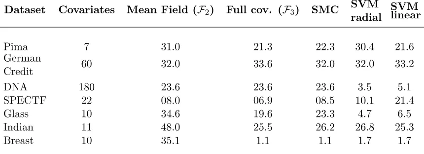
We now compare the numerical performance of the mean field and full covariance VB approximations to the Gibbs posterior (as approximated by SMC, see Section 3.1) for the classification of standard datasets; see Table 1. The datasets are all available in the UCI repository3 except for the DNA dataset which is part of the R package mlbench by Leisch and Dimitriadou (2010). When no split between the training sample is provided we split the data in half. The design matrices are centered and scaled before being used. For the Glass dataset we compare the “silicon” class against the other classes.
We also include results for a linear SVM (support vector machine) and a radial kernel SVM; the latter comparison is not entirely fair, since this is a non-linear classifier, while all the other classifiers are linear. Except for the Glass and DNA datasets, the full covariance VB approximation performs as well as or better than both SMC and SVM (while being much faster to compute, especially compared to SMC). Note that some high errors for the VB approximations can be due to the fact that the optimization of the objective is harder (we address this issue in next section).
Interestingly, VB outperforms SMC in certain cases. This might be due to the fact that a VB approximation tends to be more concentrated around the mode than the Gibbs posterior it approximates. Mean field VB does not perform so well on certain datasets (e.g. Indian). This may due either to the approximation family being too small, or to the corresponding optmisation problem to be strongly multi-modal. We address this issue in next section.
6. Application to classification under convexified loss
Compared to the previous section, the advantage of convex classification is that the cor-responding variational approximation will amount to minimizing a convex function. This
Dataset Covariates Mean Field (F2) Full cov. (F3) SMC SVM radial
SVM linear
Pima 7 31.0 21.3 22.3 30.4 21.6
German
Credit 60 32.0 33.6 32.0 32.0 33.2
DNA 180 23.6 23.6 23.6 3.5 5.1
SPECTF 22 08.0 06.9 08.5 10.1 21.4
Glass 10 34.6 19.6 23.3 4.7 6.5
Indian 11 48.0 25.5 26.2 26.8 25.3
Breast 10 35.1 1.1 1.1 1.7 1.7
Table 1: Comparison of misclassification rates (%).
Misclassification rates for different datasets and for the proposed approximations of the Gibbs posterior. The last two columns are the missclassification rate given by a SVM with radial kernel and a linear SVM. The hyper-parameters are chosen by cross-validation.
means that (a) the minimization problem will be easier to deal with; and (b) we will be able to compute a bound for the integrated risk after a given number of steps of the minimization procedure.
The setting is the same as in the previous section, except that for convenience we now take Y={−1,1}, and the risk is based on the hinge loss,
rHn(θ) = 1
n
n X
i=1
max(0,1−Yihθ, Xii).
We will write RH for the theoretical counterpart and ¯RH for its minimum in θ. We keep the superscriptH in order to allow comparison with the riskRunder the 0-1 loss. We assume in this section that the Xi are uniformly bounded, that is, we have almost surely kXik∞= maxj|Xi,j|< cx for some cx >0. Note that we do not require an assumption of the form (A1) to obtain the results of this section, as we rely directly on the Lipschitz continuity of the hinge risk.
6.1 Theoretical Results
Contrary to the previous section, the risk is not bounded in θ, and we must specify a prior distribution for the Hoeffding assumption to hold.
Lemma 3 Under an independent Gaussian prior π such that each component is N(0, ϑ2), and for λ < c1
x
q n ϑ
2 and with bounded design |X
ij|< cx, Hoeffding assumption (1) is
satisfied with f(λ, n) =λ2/(4n)−1 2log
1−ϑ2λ2c2x
2n
The main impact of such a bound is that the prior variance cannot be taken too big relative toλ.
Corollary 6.1 Assume that the VB approximation is done on either F1, F2 or F3. Take
λ= c1
x
pn
ϑ2 and ϑ= √1
d. For any ε >0, with probability at least 1−ε we have
simultane-ously
R
RHd ˆρλ R
RHd ˜ρ λ
≤RH+cx 2
r
d nlog
n d +cx
d n
r
d n +
1 √
nd
2c2x+ 1 2cx
+ 2cxlog 2
The oracle inequality in the above corollary enjoys the same rate of convergence as the equivalent result in the preceding section. In the following we link the two results.
Remark 6.1 As stated in the beginning of the section we can use the estimator specified under the hinge loss to bound the excess risk of the 0-1 loss. We write R? and RH? the respective risk for their corresponding Bayes classifiers. From Zhang (2004) (section 3.3) we have the following inequality, linking the excess risk under the hinge loss and the 0-1
loss,
R(θ)−R?≤RH(θ)−RH?
for every θ ∈ Rp. By integrating with respect to ρ˜H (the VB approximation on any
F1,F2,F3 of the Gibbs posterior for the hinge risk) and making use of Corollary 6.1 we
have with high probability,
˜
ρH(R(θ))−R? ≤ inf θ∈RpR
H(θ)−RH?+O r
d nlog
n
d
!
.
6.2 Numerical application
We have motivated the introduction of the hinge loss as a convex upper bound. In the sequel we show that the resulting VB approximation also leads to a convex optimization problem. This has the advantage of opening a range of possible optimization algorithms (Nesterov, 2004). In addition we are able to bound the error of the approximated measure after a fixed number of iterations (see Theorem 6.2).
Under the modelF1 each individual risk is given by:
ρm,σ(ri(θ)) = (1−Γim) Φ
1−Γim
σkΓik2
+σkΓikϕ
1−Γim
σkΓik2
:= Ξi
m
σ
,
Hence the lower bound to be maximized is given by
L(m, σ) =−λ
n
( n X
i=1
(1−Γim) Φ
1−Γim
σkΓik2
+ n X
i=1
σkΓikϕ
1−Γim
σkΓik2 )
−kmk 2 2 2ϑ +
d
2
logσ2− ϑ
σ2
.
It is easy to see that the function is convex in (m, σ), first note that the map
Ψ :
x y
7→xΦ
x y +yϕ x y ,
is convex and note that we can write Ξi m σ = Ψ A x y +b
hence by
compo-sition of convex function with linear mappings we have the result. Similar reasoning could be held for the case F2 and F3, where in later the parametrization should be done in C such that Σ = CCt. The bound is however not universally Lipschitz in σ, this impacts the optimization algorithms. In Theorem 6.2 we define a ball around the optimal value of the objective, containing the initial values. We denote it’s radius by M. On this ball the objective is Lipschitz (with coefficient L) and optimal convex solvers can be used (e.g. Nesterov (2004) section 3.2.3).
On the class of function F0 = n
Φm,1
n,m
∈Rdo, for which our Oracle inequalities still hold we could get faster numerical algorithms. The objective function has Lipschitz continuous derivatives and we would get a rate of (1+k)L 2.
Other convex loss could be considered which could lead to convex optimization prob-lems. For instance one could consider the exponential loss.
Theorem 6.2 Assume that the VB approximation is based on eitherF1,F2 or F3. Denote by ρ˜k(dθ)the VB approximated measure after the kth iteration of an optimal convex solver using the hinge loss. Fix M >0 large enough so that the optimal approximated mean and variance m¯,Σ¯ are at distance at most M from the initial value used by the solver. Take
λ=√nd and ϑ= √1
d then under the hypothesis of Corollary 6.1 with probability 1− Z
RHd ˜ρk≤R H
+√LM 1 +k+
cx 2 r d nlog n d +cx
d n r d n+ 1 √ nd
2c2x+ 1 2cx
+ 2cxlog 2
where L is the Lipschitz coefficient on a ball of radius M defined above.
Note that this result is stronger and more practical than the previous ones: it ensures a certain error level (with fixed probability 1−) for the k-th iterate of the optimization algorithm, for a known value of k. In contrast, previous results applied to the output of the optimizer ”fork large enough”.
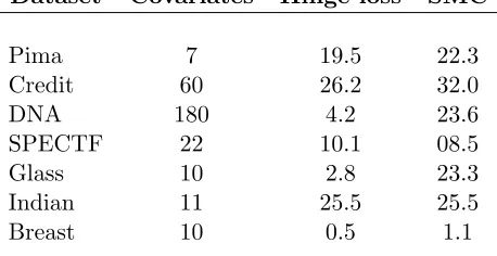
Dataset Covariates Hinge loss SMC
Pima 7 19.5 22.3
Credit 60 26.2 32.0
DNA 180 4.2 23.6
SPECTF 22 10.1 08.5
Glass 10 2.8 23.3
Indian 11 25.5 25.5
Breast 10 0.5 1.1
Table 2: Comparison of misclassification rates (%).
Misclassification rates for different datasets and for the proposed approximations of the Gibbs posterior. The hyperparameters are chosen by cross-validation. This is to be compared to Table 1. The variational Bayes approximation was computed using the R package we developed (see the introduction for a reference).
7. Application to ranking
7.1 Preliminaries
We now focus on the ranking problem. We follow Cl´emen¸con et al. (2008) for the definitions of the basic concepts: Y = {0,1}, Θ = X = Rd and fθ : X2 → {−1,+1} for θ ∈ Θ;
fθ(x, x0) = 1 (resp. −1) means that x is more (resp. less) likely to correspond to label 1 thanx0. The natural risk function is then
R(θ) =P[(Y1−Y2)fθ(X1, X2)<0] and the empirical risk
rn(θ) = 1
n(n−1) X
1≤i6=j≤n
1{(Yi−Yj)fθ(Xi,Xj)<0}.
Again, we recall classical results.
Lemma 4 The Hoeffding-type assumption is satisfied withf(λ, n) = nλ−21.
The variant of the margin assumption adapted to ranking was established by Robbiano (2013) and Ridgway et al. (2014).
Lemma 5 Assume the following margin assumption:
E[(1fθ(X1,X2)[Y1−Y2]<0−1fθ(X1,X2)[Y1−Y2]<0)
2]≤C[R(θ)−R].
We focus on linear classifiers,fθ(x, x0) =−1 + 2×1hθ,xi>hθ,x0i. Like in the classification
setting, hx, θi is interpreted as a score related to the probability that Y = 1|X = x. We consider a Gaussian prior
π(dθ) = d Y
i=1
ϕ(θi; 0, ϑ2)dθi
and the approximation families will be the same as in Section 5: F1={Φm,σ2,m∈Rd, σ2 ∈ R∗+},F2={Φm,σ2,m∈Rd,σ2 ∈(R∗+)2}and F3 ={Φm,Σ,m∈Rd,Σ∈ Sd+}.
7.2 Theoretical study
Here again, we start with the empirical bound.
Corollary 7.1 For any ε > 0, with probability at least 1−ε we have, for any m ∈ Rd,
σ2 ∈(R+)d,
Z
RdΦm,σ2 ≤
Z
rndΦm,σ2 +
λ n−1+
1 2
Pd j=1
h logϑσ22
i
+σ2i
ϑ2
i
+ k2ϑmk22 −d2 + log 1ε
λ .
In order to derive a theoretical bound, we introduce the following variant of Assump-tion A1.
Definition 7.1 We say that Assumption A2 is satisfied when there is a constantc >0such that, for any(θ, θ0)∈Θ2 withkθk=kθ0k= 1,P(hX1−X2, θi hX1−X2, θ0i<0)≤ckθ−θ0k. Assumption A2 is just Assumption A1 applied to the distribution of (X1−X2). Intuitively, it means that two parameters close to each other rank X1 and X2 in the same way (with large probability).
Corollary 7.2 Use either F1, F2 or F3. Take λ= q
d(n−1)
2 and ϑ= 1. Under (A2), for
any ε >0, with probability at least 1−ε,
R
Rd ˆρλ R
Rd ˜ρλ
≤R+ r
2d n−1
1 +1
2log (2d(n−1))
+ c √
2 √
n−1+
1
(n−1)3/2√2d+
2√2 log 2eε p
(n−1)d .
Finally, under an additional margin assumption, we have:
Corollary 7.3 Under Assumption A2 and the margin assumption of Lemma (5), for λ= n−1
C+5 and ϑ >0, for any ε >0, with probability at least 1−ε, R
Rd ˆρλ R
Rd ˜ρλ
≤R¯+(C+ 5)(C+ 1) 2
dlogn ϑ
n−1 +
dϑ n(n−1)+
1
ϑ− d ϑn−1 +
2
n−1log 2
ε
+ √
d4c(C+ 1)
It is possible to optimize the bound with respect toϑ. The proof is similar to the ones of Corollaries 5.2, 5.3 and 7.2.
As in the case of classification, ranking under an AUC loss can be done by replacing the indicator function by the corresponding upper bound given by an hinge loss. In this case we can derive similar results as for the convexified classification in particular we can get a convex minimization problem and obtain result without requiring assumption (A2).
7.3 Algorithms and numerical results
As an illustration we focus here on family F2 (mean field). In this case the VB objective to maximize is given by:
L(m, σ2) =− λ
n+n−
X
i:yi=1,j:yj=0
Φ
−q Γijm Pd
k=1(γijk)2σk2
− kmk2
2 2ϑ +
1 2
d X
k=1
logσk2−σ 2 k
ϑ
,
(7) where Γij = Xi−Xj, n+ = card{1 ≤i≤ n: Yi = 1}, n− =n−n+ = card{1 ≤i≤ n:
Yi= 0}and where (γijk)k are the elements of Γ.
This function is expensive to compute, as it involvesn+n− terms, the computation of
which is O(p).
We propose to use a stochastic gradient descent in the spirit of Hoffman et al. (2013). The model we consider is not in an exponential family, meaning we cannot use the trick developed by these authors. We propose instead to use a standard descent.
The idea is to replace the gradient by a unbiased version based on a batch of size B
as described in Algorithm 4 in the Appendix. Robbins and Monro (1951) show that for a step-size (λt)t such that Ptλ2t <∞ and
P
tλt =∞ the algorithm converges to a local optimum.
In our case we propose to sample pairs of data with replacement and use the unbiased version of the derivative of the risk component. We use a simple gradient descent without any curvature information. One could also use recent research on stochastic quasi Newton-Raphson (Byrd et al., 2014).
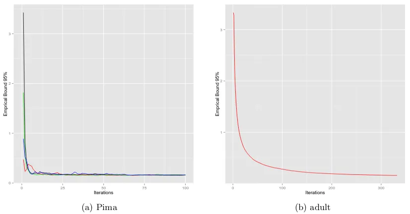
For illustration, we consider a small dataset (Pima), and a larger one (Adult). Both datasets are available in the UCI repository4. As for the previous experiment the data is scaled and centered. The latter is already quite challenging with n+n− = 193,829,520
pairs to compare. In both cases with different size of batches convergence is obtained with a few iterations only and leads to acceptable bounds.
In Figure 1 we show the empirical bound on the AUC risk as a function of the iteration of the algorithm, for several batch sizes. The bound is taken for 95% probability, the batch sizes are taken to be B = 1,10,20,50 for the Pima dataset, and 50 for the Adult dataset. The figure shows an additional feature of VB approximation in the context of
0 1 2 3
0 25 50 75 100
Iterations
Empr
ical Bound 95%
(a) Pima
1 2 3
0 100 200 300
Iterations
Empr
ical Bound 95%
(b) adult
Figure 1: Error bound at each iteration, stochastic descent, Pima and Adult datasets.
Stochastic VB with fixed temperatureλ= 100 for Pima andλ = 1000 for adult. The left panel shows
several curves that correspond to different batch sizes; these curves are hard to distinguish. The right panel
is for a batch size of 50. The adult dataset hasn= 32556 observation and n+n− = 193829520 possible
pairs. The convergence is obtained in order of seconds. The bounds are the empirical bounds obtained in Corollary 7.1 for a probability of 95%.
Gibbs posterior: namely the possibility of computing the empirical upper bound given by Corollary 7.1. That is we can check the quality of the bound at each iteration of the algorithm, or for different values of the hyperparameters.
8. Application to matrix completion
We observe i.i.d. pairs ((Xi, Yi))ni=1 where Xi ∈ {1, . . . , m1} × {1, . . . , m2}, and we assume that there is a m1×m2-matrix M such thatYi=MXi+εi and theεi are centred.
Assuming that Xi is uniform on{1, . . . , m1} × {1, . . . , m2}, thatfθ(Xi) =θXi, and taking
the quadratic risk, R(θ) =E(Yi−θXi)
2
, we have that
R(θ)−R = 1
m1m2
kθ−Mk2F where k·kF stands for the Frobenius norm.
A common way to parametrize the problem is
Θ ={θ=U VT, U ∈Rm1×K, V ∈
Rm2×K}
where K is large; e.g. K = min(m1, m2). Following Salakhutdinov and Mnih (2008), we define the following prior distribution: U·,j ∼ N(0, γjI), V·,j ∼ N(0, γjI) where the γj’s are i.i.d. from an inverse gamma distribution,γj ∼ IΓ(a, b).
Note that VB algorithms were used in this context by Lim and Teh (2007) (with a slightly simpler prior however: the γj’s are fixed rather than random). Since then, this prior and variants were used in several papers (e.g. Lawrence and Urtasun, 2009; Zhou et al., 2010). Until now, no theoretical results were proved to the best of our knowledge. Two papers prove minimax-optimal rates for slightly modified estimators (by truncation), for which efficient algorithms are unknown (Mai and Alquier, 2015; Suzuki, 2014). However, using Theorems 4.2 and 4.3 we are able to prove the following: if there is a PAC-Bayesian bound leading to a rate for ˆρλ in this context, then the same rate holds for ˜ρλ. In other words: if someone proves the conjecture that the Gibbs estimator is minimax-optimal (up to log terms) in this context, then the VB approximation will enjoy automatically the same property.
We propose the following approximation:
F =
ρ(d(U, V)) = m1
Y
i=1
ui(dUi,·)
m2
Y
j=1
vj(dVj,·)
.
Theorem 8.1 Assume thatM =U VT with|U
i,k|,|Vj,k|≤C. Assume thatrank(M) =rso
that we can assume thatU·,r+1=· · ·=U·,K =V·,r+1=· · ·=V·,K = 0(note that the priorπ
does not depend on the knowledge ofr though). Choose the prior distribution on the hyper-parameters γj as inverse gammaInv−Γ(a, b) withb≤1/[2β(m1∨m2) log(2K(m1∨m2))].
Then there is a constant C(a, C) such that, for any β >0,
inf
ρ∈FK(ρ, πβ)≤ C(a, C)
r(m1+m2) log [βb(m1+m2)K] + 1
β
.
For instance, in Theorem 4.3, in classification and ranking we had λ, λ−g(λ, n) and
λ+g(λ, n) of orderO(n). In this case we would have:
2
λ−g(λ, n)ρinf∈FK
ρ, πλ+g(λ,n) 2
=O
C(a, C)r(m1+m2) log [nb(m1+m2)K]
n
,
and note that in this context it is know that the minimax rate is at least r(m1+m2)/n (Koltchinskii et al., 2011).
8.1 Algorithm
As already mentioned, the approximation family is not parametric in this case, but rather of type mean field. The corresponding VB algorithm amounts to iterating equation (4), which takes the following form in this particular case:
uj(dUj,.)∝exp (
−λ
n
X
i
EV,U−j
(YXi−(U V
T) Xi)
2 −
K X
k=1
Eγj
1 2γk
Ujk2
)
vj(dVj,.)∝exp (
−λ
n
X
i
EV−j,U
(YXi−(U V
T) Xi)
2 −
K X
k=1
Eγj
1 2γk
Vjk2
)
p(γk)∝exp
− 1
2γk
X
j
EUUkj2 + X
i
EVVik2
+ (α+ 1) log 1
γk − β
γk
where the expectations are taken with respect to the thus defined variational approxi-mations. One recognises Gaussian distributions for the first two, and an inverse Gamma distribution for the third. We refer to Lim and Teh (2007) for more details on this al-gorithm and for a numerical illustration. However, we point out that in this case, while the algorithm seems to work well in practice, there is no theoretical guarantee that it will converge to the global minimum of the problem.
9. Discussion
We showed in several important scenarios that approximating a Gibbs posterior through VB (Variational Bayes) techniques does not deteriorate the rate of convergence of the corresponding procedure. We also described practical algorithms for fast computation of these VB approximations, and provided empirical bounds that may be computed from the data to evaluate the performance of the so-obtained VB-approximated procedure. We believe these results provide a strong incentive to recommend VB as the default approach to approximate Gibbs posteriors, in lieu of Monte Carlo methods. We also developed a R package5 for convexified losses (classification and bipartite ranking), applying the ideas of Section 6.
We hope to extend our results to other applications beyond those discussed in this paper, such as regression. One technical difficulty with regression is that the risk function is not bounded, which makes our approach a bit less direct to apply. In many papers on PAC-Bayesian bounds for regression, the noise can be unbounded (usually, it is assumed to be sub-exponential), but one assumes that the predictors are bounded, see e.g. Alquier and Biau (2013). However, using the robust loss function of Audibert and Catoni, it is possible to relax this assumption (Audibert and Catoni, 2011; Catoni, 2012). This requires a more technical analysis, which we leave for further work.
Appendix A. Proofs
A.1 Preliminary remarks
Direct calculation yields, for anyρπ withRrndρ <∞,
K(ρ, π[rn]) =λ
Z
rndρ+K(ρ, π) + log Z
exp(−h)dπ.
Two well known consequences are
π[h] = arg min ρ∈M1
+(Θ)
Z
hdρ+K(ρ, π)
,
−log Z
exp(−h)dπ = min ρ∈M1
+(Θ)
Z
hdρ+K(ρ, π)
.
We will use these inequalities many times in the followings. The most frequent application will be with h(θ) =λrn(θ) (in this caseπ[λrn] = ˆρλ) or h(θ) =±λ[rn(θ)−R(θ)], the first case leads to
K(ρ,ρˆλ) =λ
Z
rndρ+K(ρ, π) + log Z
exp(−λrn)dπ, (8)
ˆ
ρλ = arg min ρ∈M1
+(Θ)
λ
Z
rndρ+K(ρ, π)
, (9)
−log Z
exp(−λrn)dπ = min ρ∈M1
+(Θ)
λ
Z
rndρ+K(ρ, π)
. (10)
We will use (8), (9) and (10) several times in this appendix.
A.2 Proof of the theorems in Subsection 4.1
Proof of Theorem 4.1. This proof follows the standard PAC-Bayesian approach (see Catoni (2007)). Apply Fubini’s theorem to the first inequality of (1):
E
Z
then apply the preliminary remark with h(θ) =λ[rn(θ)−R(θ)]:
Eexp
( sup ρ∈M1
+(Θ)
Z
λ[R(θ)−rn(θ)]ρ(dθ)− K(ρ, π)−f(λ, n) )
≤1.
Multiply both sides by εand useE[exp(U)]≥P(U >0) for anyU to obtain:
P
" sup ρ∈M1
+(Θ)
Z
λ[R(θ)−rn(θ)]ρ(dθ)− K(ρ, π)−f(λ, n) + log(ε)>0 #
≤ε.
Then consider the complementary event:
P
∀ρ∈ M1
+(Θ), λ Z
Rdρ≤λ
Z
rndρ+f(λ, n) +K(ρ, π) + log
1
ε
≥1−ε.
Proof of Theorem 4.2. Using the same calculations as above, we have, with probability at least 1−ε, simultaneously for all ρ∈ M1
+(Θ),
λ
Z
Rdρ≤λ
Z
rndρ+f(λ, n) +K(ρ, π) + log
2
ε
(11)
λ
Z
rndρ≤λ
Z
Rdρ+f(λ, n) +K(ρ, π) + log
2
ε
. (12)
We use (11) withρ= ˆρλ and (9) to get
λ
Z
Rd ˆρλ≤ inf ρ∈M1
+(Θ)
λ
Z
rndρ+f(λ, n) +K(ρ, π) + log
2
ε
and plugging (12) into the right-hand side, we obtain
λ
Z
Rd ˆρλ ≤ inf ρ∈M1
+(Θ)
λ
Z
Rdρ+ 2f(λ, n) + 2K(ρ, π) + 2 log
2
ε
.
Now, we work with ˜ρλ = arg minρ∈FK(ρ,ρˆλ). Plugging (8) into (11) we get, for any ρ,
λ
Z
Rdρ≤f(λ, n) +K(ρ,ρˆλ)−log Z
exp(−λrn)dπ+ log
2
ε
.
By definition of ˜ρλ, we have:
λ
Z
Rd ˜ρλ≤ inf ρ∈F
f(λ, n) +K(ρ,ρˆλ)−log Z
exp(−λrn)dπ+ log
2
ε
and, using (8) again, we obtain:
λ
Z
Rd ˜ρλ ≤ inf ρ∈F
λ
Z
rndρ+f(λ, n) +K(ρ, π) + log
2
ε
.
We plug (12) into the right-hand side to obtain:
λ
Z
Rd ˜ρλ ≤ inf ρ∈F
λ
Z
Rdρ+ 2f(λ, n) + 2K(ρ, π) + 2 log
2
ε
.
This proves the second inequality of the theorem. In order to prove the claim
Bλ(F) =Bλ(M1
+(Θ)) + 2
λρinf∈FK(ρ, πλ2
),
note that
Bλ(F) = inf ρ∈F
( Z
Rdρ+2f(λ, n)
λ +
2K(ρ, π)
λ +
2 log 2ε
λ ) = inf ρ∈F ( −2 λlog Z exp −λ 2R
dπ+2f(λ, n)
λ +
2K(ρ, πλ
2)
λ +
2 log 2ε
λ
)
=−2
λlog Z exp −λ 2R
dπ+ 2f(λ, n)
λ +
2 log 2ε
λ +
2
λρinf∈FK(ρ, πλ2)
=Bλ(M1
+(Θ)) + 2
λρinf∈FK(ρ, πλ2
).
This ends the proof.
A.3 Proof of Theorem 4.3 (Subsection 4.2)
Proof of Theorem 4.3. As in the proof of Theorem 4.1, we apply Fubini, then (10) to the first inequality of (2) to obtain
Eexp sup ρ Z
λ[R(θ)−R]−λ[rn(θ)−rn]−g(λ, n)[R(θ)−R]
ρ(dθ)− K(ρ, π)
≤1
and we multiply both sides byε/2 to get
P
( sup
ρ "
[λ−g(λ, n)] Z
Rdρ−R
≥λ
Z
rndρ−rn
+K(ρ, π) + log
2
ε
#) ≤ ε
2. (13)
We now consider the second inequality in (2):
The same derivation leads to P ( sup ρ "
[λ−g(λ, n)] Z
rndρ−rn
≥λ
Z
Rdρ−R
+K(ρ, π) + log
2
ε
#) ≤ ε
2. (14)
We combine (13) and (14) by a union bound argument, and we consider the complementary event: with probability at least 1−ε, simultaneously for all ρ∈ M1
+(Θ), [λ−g(λ, n)]
Z
Rdρ−R
≤λ
Z
rndρ−rn
+K(ρ, π) + log 2 ε , (15) λ Z
rndρ−rn
≤[λ+g(λ, n)] Z
Rdρ−R
+K(ρ, π) + log
2
ε
. (16)
We now derive consequences of these two inequalities (in other words, we focus on the event where these two inequalities are satisfied). Using (9) in (15) yields
[λ−g(λ, n)] Z
Rd ˆρλ−R
≤ inf ρ∈M1
+(Θ)
λ
Z
rndρ−rn
+K(ρ, π) + log
2
ε
.
We plug (16) into the right-hand side to obtain:
[λ−g(λ, n)] Z
Rd ˆρλ−R
≤ inf ρ∈M1
+(Θ)
(
[λ+g(λ, n)] Z
Rdρ−R
+ 2K(ρ, π) + 2 log
2
ε
)
.
Now, we work with ˜ρλ. Plugging (8) into (13) we get
[λ−g(λ, n)] Z
Rdρ−R
≤ K(ρ,ρˆλ)−log Z
exp[−λ(rn−rn)]dπ+ log
2
ε
.
By definition of ˜ρλ, we have:
[λ−g(λ, n)] Z
Rd ˜ρλ−R
≤ inf ρ∈F
K(ρ,ρˆλ)−log Z
exp[−λ(rn−rn)]dπ+ log
2
ε
.
Then, apply (8) again to get:
[λ−g(λ, n)] Z
Rd ˜ρλ−R ≤ inf ρ∈F λ Z
(rn−rn)dρ+K(ρ, π) + log
2
ε
Plug (16) into the right-hand side to get
[λ−g(λ, n)] Z
Rd ˜ρλ−R
≤ inf ρ∈F
[λ+g(λ, n)] Z
(R−R)dρ+ 2K(ρ, π) + 2 log 2 ε .
A.4 Proofs of Section 5
Proof of Lemma 1. Combine Theorem 2.1 p. 25 and Lemma 2.2 p. 27 in Boucheron et al.
(2013).
Proof of Lemma 2. Apply Theorem 2.10 in Boucheron et al. (2013), and plug the margin assumption.
Proof of Corollary 5.2. We remind that thanks to (6) it is enough to prove the claim for F1. We apply Theorem 4.2 to get:
Bλ(F1) = inf (m,σ2)
( Z
RdΦm,σ2 +
λ n+ 2
K(Φm,σ2, π) + log 2ε
λ
)
= inf (m,σ2)
Z
RdΦm,σ2+
λ n+ 2
d h 1 2log ϑ2 σ2 +2ϑσ22
i
+k2ϑmk22 −
d 2 + log
2 ε λ .
Note that the minimizer ofR,θ, is not unique (becausefθ(x) does not depend onkθk) and we can chose it in such a way thatkθk= 1. Then
R(θ)−R=E
h
1hθ,XiY <0−1hθ,XiY <0 i
≤E
h
1hθ,Xihθ,Xi<0 i
=P hθ, Xiθ, X<0≤c
θ
kθk−θ
≤2ckθ−θk.
So:
Bλ(F1)≤R+ inf (m,σ2)
2c
Z
kθ−θkΦm,σ2(dθ)
+λ
n+ 2
dh12logϑσ22
+2ϑσ22
i
+k2ϑmk22 −d2 + log 2ε
λ
.
We now restrict the infimum to distributions ν such thatm=θ:
B(F1)≤R+ inf σ2 2c √
dσ+λ
n+ dlog ϑ2 σ2
+dσϑ22 +ϑ12 −d+ 2 log 2ε
We putσ = 2λ1 and substitute √1
d forϑ to get
B(F1)≤R+ λ
n+
c√d+dlog(4λd2) + 4λd22 + 2 log 2ε
λ .
Substitute√nd forλto get the desired result.
Proof of Corollary 5.3. We apply Theorem 4.3:
Z
(R−R)d ˜ρλ
≤ inf m,σ2
λ+g(λ, n)
λ−g(λ, n) Z
(R−R¯)dΦm,σ2 +
1
λ−g(λ, n)
2K(Φm,σ2, π) + 2 log
2
whereλ < C+12n . Computations similar to those in the the proof of Corollary 5.2 lead to Z
Rdρ˜λ ≤R+ inf m,σ2
(
2cλ+g(λ, n) λ−g(λ, n)
Z
kθ−θkΦm,σ2(dθ)
+ 2 1 2
Pd j=1
h logϑσ22
+σϑ22
i
+k2ϑmk22 −d2 + log 2ε
λ−g(λ, n)
)
.
taking m= ¯θ and λ= C+22n , we get the result.
A.5 Proofs of Section 6
Proof of Lemma 3. For fixed θwe can upper bound the individual risk such that:
0≤max(0,1−< θ, Xi > Yi)≤1 +|< θ, Xi >|
such that we can apply Hoeffding’s inequality conditionally on Xi and fixed θ. We get,
Eexp λ(RH −rHn)
|X1,· · ·, Xn
≤exp (
λ2
8n2 n X
i=1
(1 +|< θ, Xi>|)2 )
≤exp
λ2
4n+ λ2c2x
4n kθk
2
respect to theXi’s and with respect to our Gaussian prior.
π
Eexp λ(RH −rHn) ≤
expλ4n2 (2π)d2
√
ϑ2 Z
exp
λ2c2x
4n kθk
2− 1 2ϑ2kθk
2
dθ
≤
expλ4n2 (2π)d2
√ ϑ2 Z exp −1 2 1
ϑ2 −
λ2c2x
2n
kθk2
dθ
The integral is a properly defined Gaussian integral under the hypothesis that ϑ12−
λ2c2
x
2n >0 hence λ < c1
x
q n ϑ
2. The integral is proportional to a Gaussian and we can directly write:
πEexp λ(RH −rnH) ≤
expλ4n2 q
1−ϑ2λ2c2x
2n writing everything in the exponential gives the desired result.
Proof of Corollary 6.1. We apply Theorem 4.2 to get:
Bλ(F1) = inf (m,σ2)
( Z
RHdΦm,σ2+
λ
2n−
1
λlog
1−ϑ
2λ2c2 x 2n
+ 2K(Φm,σ2, π) + log 2 ε λ ) = inf (m,σ2)
Z
RHdΦm,σ2 +
λ
2n−
1
λlog
1− ϑλ
2c2 x 2n + 2 1 2 Pd j=1 h logϑσ22
+σϑ22
i
+k2ϑmk22 −d2 + log 2ε
λ .
We use the fact that the hinge loss is Lipschitz and that the (Xi) are uniformly bounded kXk∞< cx. We getRH(θ)≤R¯H+cx
√
dkθ−θ¯k and restrict the infemum to distributions
ν such thatm=θ:
B(F1)≤RH+inf σ2
cxdσ2+
λ
2n−
1
λlog
1−ϑ
2λ2c2 x 2n + dlog ϑ2 σ2
+dσϑ22 +ϑ12 −d+ 2 log 2ε
λ .
We specify σ2= √1
dn and λ=cx p n
ϑ2 such that we get:
B(F1)≤RH+c x r d n+ √ ϑ2 2cx
√
n−cx
r
ϑ2
n log
1−1
2
+dc√xϑ
nlog
ϑ2
√
nd+cxϑ d
nϑ2 +ϑ12 −d+ 2 log 2ε
√
n .
To get the correct rate we take the prior variance to be ϑ2 = 1
Proof of Theorem 6.2. From Nesterov (2004) (th. 3.2.2) we have the following bound on the objective function minimized by VB, (the objective is not uniformlly Lipschitz)
ρk(rnH) + 1
λK(ρ
k, π)− inf ρ∈F1
ρ(rnH) + 1
λK(ρ, π)
≤ √LM
1 +k. (17)
We have from equation (11) specified for measuresρk probability 1−ε,
λ
Z
rHndρk≤λ
Z
RHdρk+f(λ, n) +K(ρk, π) + log
1
ε
Combining the two equations yields,
Z
RHdρk≤ √LM 1 +k+
1
λf(n, λ) + infρ∈F1
ρ(rnH) + 1
λK(ρ, π)
+1
λlog
1
ε
We can therefore write for any ρ∈ F1, Z
RHdρk≤ √LM 1 +k+
1
λf(n, λ) +ρ(r
H n) +
1
λK(ρ, π) +
1
λlog
1
ε
Using equation (11) a second time we get with probability 1−ε
Z
RHdρk≤ √LM 1 +k +
2
λf(n, λ) +ρ(R
H) + 2
λK(ρ, π) +
2
λlog
2
ε
Because this is true for anyρ∈ F1in 1−εwe can write the bound for the smallest measure inF1.
Z
RHdρk ≤ √LM 1 +k+
2
λf(n, λ) + infρ∈F1
ρ(RH) + 2
λK(ρ, π)
+ 2
λlog
2
ε
By taking the Gaussian measure with variance n1 and mean θ in the infimum and taking
λ= c1
x
√
nd and ϑ= 1d, we can use the results of Corollary 6.1 to get the result.
A.6 Proofs of Section 7
Proof of Lemma 4. The idea of the proof is to use Hoeffding’s decomposition of U-statistics combined with Hoeffding’s inequality for iid random variables. This was done in ranking by Cl´emen¸con et al. (2008), and later in Robbiano (2013); Ridgway et al. (2014) for ranking via aggregation and Bayesian statistics. The proof is as follows: we define
so that
Un:= 1
n(n−1) X
i,j
qi,jθ =rn(θ)−R(Θ).
From Hoeffding (1948) we have
Un= 1
n! X
π 1 bn 2c
bn
2c
X
i=1
qθπ(i),π(i+bn
2c)
where the sum is taken over all the permutationsπ of{1, . . . , n}. Jensen’s inequality leads to
Eexp[λUn] =Eexp
λ 1
n! X
π 1 bn 2c
bn
2c
X
i=1
qθπ(i),π(i+bn
2c)
≤ 1
n! X
π
Eexp
λ
bn 2c
bn
2c
X
i=1
qπ(i),π(i+θ bn
2c)
.
We now use, for each of the terms in the sum we use the same argument as in the proof of Lemma 1 to get
Eexp[λUn]≤ 1
n! X
π exp
λ2
2bn 2c
≤exp
λ2 n−1
(in the last step, we used bn
2c ≥(n−1)/2). We proceed in the same way to upper bound
Eexp[−λUn].
Proof of Lemma 5. As already done above, we use Bernstein inequality and Hoeffding
decomposition. Fix θ. We define this time
qi,jθ =1{hθ, Xi−Xji(Yi−Yj)<0} −1{
θ, Xi−Xj
(Yi−Yj)<0} −R(θ) +R
so that
Un:=rn(θ)−rn−R(θ) +R= 1
n(n−1) X
i6=j
qθi,j.
Then,
Un= 1
n! X
π 1 bn2c
bn
2c
X
i=1
qθπ(i),π(i+bn
Jensen’s inequality:
Eexp[λUn] =Eexp
λ 1
n! X
π 1 bn 2c
bn
2c
X
i=1
qθπ(i),π(i+bn
2c)
≤ 1
n! X
π
Eexp
λ
bn 2c
bn
2c
X
i=1
qπ(i),π(i+θ bn
2c)
.
Then, for each of the terms in the sum, use Bernstein’s inequality:
Eexp
λ
bn 2c
bn
2c
X
i=1
qπ(i),π(i+θ bn
2c)
≤exp
E((qπ(1),π(1+θ bn
2c))
2) λ2
bn
2c
2
1−2bλn
2c
.
We use againbn2c ≥(n−1)/2. Then, as the pairs (Xi, Yi) are iid, we haveE((qπ(1),π(1+θ bn
2c))
2) =
E((q1,2θ )2) and thenE((q1,2θ )2)≤C[R(θ)−R] thanks to the margin assumption. So
Eexp
λ
bn 2c
bn
2c
X
i=1
qπ(i),π(i+θ bn
2c)
≤exp
C[R(θ)−R]nλ−21
1−n4λ−1
.
This ends the proof of the proposition.
Proof of Corollary 7.2. The calculations are similar to the ones in the proof of Corollary 5.2 so we don’t give the details. Note that when we reach
Bλ(F1)≤R+ 2λ
n−1 +
c√d+dlog(2λ) +4λd2 + 2 log
2e ε
λ ,
an approximate minimization with respect to λleads to the choice λ= q
d(n−1) 2 . A.7 Proofs of Section 8
Proof. First, note that, for anyρ,
K(ρ, πβ) =β Z
(R−R)dρ+K(ρ, π) + log Z
exp−β(R−R)dπ
≤β
Z
(R−R)dρ+K(ρ, π).
uniform on{∀(i, `),|µi,`−Ui,`|≤δ}andν is uniform on{∀(j, `),|νi,`−Vj,`|≤δ}. Note that Z
(R−R)dρM,N,δ = Z
E((θX−MX)2)ρU,V,δ(dθ) ≤
Z
3E(((U VT)X −MX)2)ρU,V,δ(d(µ, ν)) + 3
Z
E(((U νT)X −(U VT)X)2)ρU,V,δ(d(µ, ν)) + 3
Z
E(((µνT)X −(U νT)X)2)ρU,V,δ(d(µ, ν)). By definition, the first term is = 0. Moreover:
Z
E(((U νT)X −(U VT)X)2)ρU,V,δ(d(µ, ν))
=
Z 1
m1m2 X
i,j "
X
k
Ui,k(νj,k−Vj,k) #2
ρU,V,δ(d(µ, ν))
≤
Z 1
m1m2 X
i,j "
X
k
Ui,k2
# " X
k
(νj,k−Vj,k)2 #
ρU,V,δ(d(µ, ν))
≤KrC2δ2.
In the same way,
Z
E(((µνT)X−(U νT)X)2)ρU,V,δ(d(µ, ν))≤
Z
kµ−Uk2Fkνk2FρU,V,δ(d(µ, ν)) ≤Kr(C+δ)2δ2.
So: Z
(R−R)dρM,N,δ ≤2Krδ2(C+δ2).
Now, let us consider the term K(ρU,V,δ, π). An explicit calculation is possible but tedious. Instead, we might just introduce the set Gδ = {θ = µνT,kµ−UkF≤ δ,kν −VkF≤ δ} and note that K(ρU,V,δ, π) ≤logπ(1Gδ). An upper bound for Gδ is calculated page 317-320
in Alquier (2014) and the result is given by (10) in this reference:
K(ρU,V,δ, π)≤4δ2+ 2kUk2F+2kNk2F+2 log(2) + (m1+m2)rlog
1
δ
r
3π(m1∨m2)K 4
!
+ 2Klog
Γ(a)3a+1exp(2)
as soon as the restriction b≤ 2m δ2
1Klog(2m1K),
δ2
2m2Klog(2m2K) is satisfied. So we obtain:
K(ρU,V,δ, πβ)≤β2Krδ2(C+δ2) + 4δ2+ 2kUk2F+2kNk2F+2 log(2) + (m1+m2)rlog
1
δ
r
3π(m1∨m2)K 4
!
+ 2Klog
Γ(a)3a+1exp(2)
ba+12a
.
Note thatkUk2
F≤C2rm1,kVk2F≤C2rm2 and K ≤m1+m2 so it is clear that the choice
δ = q
1
β andb≤
1
2β(m1∨m2) log(2K(m1∨m2)) leads to the existence of a constantC(a, C) such
that
K(ρU,V,δ, πβ)≤ C(a, C)
r(m1+m2) log [βb(m1+m2)K] + 1
β
.
Appendix B. Implementation details
B.1 Sequential Monte Carlo
Tempering SMC approximates iteratively a sequence of distribution ρλt, with
ρλt(dθ) =
1
Zt
exp (−λtrn(θ))π(dθ),
Algorithm 1 Tempering SMC
Input N (number of particles), τ ∈ (0,1) (ESS threshold), κ > 0 (random walk tuning parameter)
Init. Sampleθi0∼πξ(θ) for i= 1 to N, set t←1,λ0= 0, Z0 = 1. Loop a. Solve in λt the equation
{PN
i=1wt(θti−1)}2 PN
i=1{wt(θit−1))2}
=τ N, wt(θ) = exp[−(λt−λt−1)rn(θ)] (18)
using bisection search. If λt ≥ λT, set ZT = Zt−1× n
1 N
PN
i=1wt(θti−1) o
, and stop.
b. Resample: for i = 1 to N, draw Ait in 1, . . . , N so that P(Ait = j) =
wt(θtj−1)/PN
k=1wt(θtk−1); see Algorithm 2 in the appendix. c. Sampleθi
t∼Mt(θ Ai
t
t−1,dθ) fori= 1 toN whereMt is a MCMC kernel that leaves invariant πt; see comments below.
d. SetZt=Zt−1× n
1 N
PN
i=1wt(θti−1) o
.
The algorithm outputs a weighted sample (wiT, θTi) approximately distributed as target posterior, and an unbiased estimator of the normalizing constant ZλT.
Algorithm 2 Systematic resampling
Input: Normalised weights Wtj :=wt(θtj−1)/ PN
i=1wt(θit−1). Output: indicesAi∈ {1, . . . , N}, fori= 1, . . . , N.
a. SampleU ∼ U([0,1]).
b. Compute cumulative weights asCn=Pn
m=1N Wm. c. Sets←U,m←1.
d. For n= 1 :N
WhileCm< s dom←m+ 1.
An←m, and s←s+ 1. End For
For the MCMC step, we used a Gaussian random-walk Metropolis kernel, with a co-variance matrix for the random step that is proportional to the empirical coco-variance matrix of the current set of simulations.
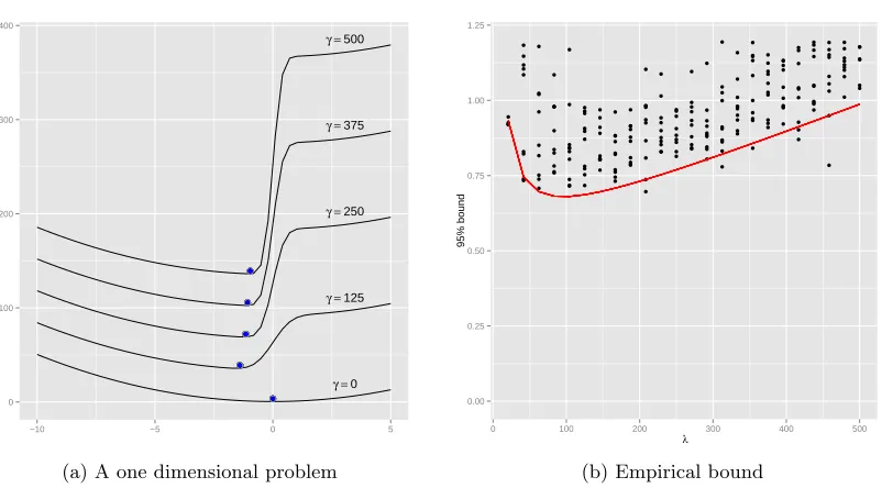
B.2 Optimizing the bound
A natural idea to find a global optimum of the objective is to try to solve a sequence of local optimization problems with increasing temperatures. For γ = 0 the problem can be solved exactly (as a KL divergence between two Gaussians). Then, for two consecutive temperatures, the corresponding solutions should be close enough.