On Differential Growth Equation to Stochastic Growth Model Using Hyperbolic Sine Function in Height/Diameter Modeling of Pines

Pure and Applied Mathematics Journal

2014; 3(5): 99-104

Published online October 10, 2014 (http://www.sciencepublishinggroup.com/j/pamj) doi: 10.11648/j.pamj.20140305.12

ISSN: 2326-9790 (Print); ISSN: 2326-9812 (Online)

On differential growth equation to stochastic growth model

using hyperbolic sine function in height/diameter modeling

of pines

Oyamakin Samuel Oluwafemi, Chukwu Angela Unna

Dept. of Statistics, University of Ibadan, Ibadan, Oyo State, Nigeria

Email address:

[email protected] (O. S. Oluwafemi), [email protected] (C. A. Unna)

To cite this article:

Oyamakin Samuel Oluwafemi, Chukwu Angela Unna. On Differential Growth Equation to Stochastic Growth Model Using Hyperbolic Sine Function in Height/Diameter Modeling of Pines. Pure and Applied Mathematics Journal. Vol. 3, No. 5, 2014, pp. 99-104.

doi: 10.11648/j.pamj.20140305.12

Abstract: Richrads growth equation being a generalized logistic growth equation was improved upon by introducing an

allometric parameter using the hyperbolic sine function. The integral solution to this was called hyperbolic Richards growth model having transformed the solution from deterministic to a stochastic growth model. Its ability in model prediction was compared with the classical Richards growth model an approach which mimicked the natural variability of heights/diameter increment with respect to age and therefore provides a more realistic height/diameter predictions using the coefficient of determination (R2), Mean Absolute Error (MAE) and Mean Square Error (MSE) results. The Kolmogorov Smirnov test and Shapiro-Wilk test was also used to test the behavior of the error term for possible violations. The mean function of top height/Dbh over age using the two models under study predicted closely the observed values of top height/Dbh in the hyperbolic Richards nonlinear growth models better than the classical Richards growth model.

Keywords: Height, Dbh, Forest, Pinus Caribaea, Hyperbolic, Richards, Stochastic

1. Introduction

Richards’s model is an extension of logistic model and was developed by Richards in (1959) simply by introducing another parameter into the Logistic growth equation, the parameter allow the shape of the upper part of the curve to be independent of the shape of the lower part, while still having an equation that tends towards an exponential form at low values of the response variable.

This additional parameter makes the Richards equation more popular. The Richards equation continues to be the most popular of the growth equations because of its flexibility; it is used for diverse purposes, including modeling tree growth, the growth of juvenile mammals and birds, and comparisons of treatment effects on plant growth.

When b = 1 the Richards equation matches the logistic equation, but for b>1 the maximum slope of the curve is Height > K/2, and when b < 1 the maximum slope of the curve is when Height < K/2. This allows a wider range of curves to be produced, but as b tends towards zero, the lowest value of Height at the point of inflexion remains greater than K/e,

where e represents the base of the natural logarithm. In fact, as b tends towards zero the Richards growth curve tends towards the Gompertz growth curve, which has its steepest slope at Height = K/e, and does not tend towards an exponential form for low Height (Richards, 1959). The model has the following differential form;

= 1 −

Sustainable forest management relies to a large extent, measure on the predictions of the future conditions of individual stands which is achieved by predicting the increment from the current stand structure and updating the current values at each cycle of iteration using a functional growth model. Trees structural changes over time can be monitored and modeled under different cutting cycles, cutting intensities and optimal management policies can be arrived at based on the results of such simulation runs.

Forest managers rely on growth and yield models to assess whether their short-term plans will meet long sustainability goals. Growth models assist forest researchers and managers in many ways. Some important uses include the ability to predict future yields and to help consider alternative cultivation practices. Models provide an efficient way to prepare resource forecasts, but a more important role may be their ability to explore management options and silvicultural alternatives EK, A.R., E.T. Birdsall, and R.J.Spear (1984) Oyamakin & Chukwu (2014) assert that g

provide a reliable way to examine silvicultural and harvesting options, to determine the sustainable timber yield, and examine the impacts of forest management and harvesting on other values of the forest. Forest managers may require information on the present status of the resource (e.g. numbers of trees by species and sizes for selected strata), forecasts of the nature and timing of future harvests, and estimates of the maximum sustainable harvest. Forest simulation models or forest growth models are very useful for forest managers and forestry researchers in many respects. A forest growth model aims to describe the dynamics of the forest closely and precisely enough to meet the needs of the f

researcher.

The total height (Ht) of a tree is important for

and estimating tree volume, stand characteristics and features through site index, but accurate measurement of this variable is time consuming. As a result, foresters often choose to measure only a few trees’ heights and estimate the remaining heights with height-diameter equations. Foresters can also use height-diameter equations to indirectly estimate height growth by applying the equations to a sequence of diameters that were either measured directly in a continuous inventory or predicted indirectly by a diameter-growth equation

1993). The diameter-growth prediction method in modeling growth and yield of trees

approximations in measuring the diameter of trees (1967) investigated several equations for Douglas included tree diameter outside bark at breast height (D an explanatory variable.

In this paper, an alternative nonlinear growth model called the hyperbolic Richards growth model was introduced and compared with the existing classical Richards

an improvement on the logistic growth model.

of the well-known features in biological creatures (Burkhart and Strub, 1974). It describes the changing size of something over time.

Sustainable forest management relies to a large extent, easure on the predictions of the future conditions of individual stands which is achieved by predicting the increment from the current stand structure and updating the current values at each cycle of iteration using a functional ral changes over time can be monitored and modeled under different cutting cycles, cutting intensities and optimal management policies can be arrived at based on the results of such simulation runs.

Forest managers rely on growth and yield models to assess term plans will meet long-term sustainability goals. Growth models assist forest researchers and managers in many ways. Some important uses include the ability to predict future yields and to help consider alternative ices. Models provide an efficient way to prepare resource forecasts, but a more important role may be their ability to explore management options and silvicultural alternatives EK, A.R., E.T. Birdsall, and R.J.Spear (1984), that growth models provide a reliable way to examine silvicultural and harvesting options, to determine the sustainable timber yield, and examine the impacts of forest management and harvesting on other values of the forest. Forest managers may require formation on the present status of the resource (e.g. numbers of trees by species and sizes for selected strata), forecasts of the nature and timing of future harvests, and estimates of the maximum sustainable harvest. Forest simulation models or owth models are very useful for forest managers and forestry researchers in many respects. A forest growth model aims to describe the dynamics of the forest closely and precisely enough to meet the needs of the forester or forestry

ight (Ht) of a tree is important for computing stand characteristics and features through site index, but accurate measurement of this variable is time consuming. As a result, foresters often choose to heights and estimate the remaining diameter equations. Foresters can also use diameter equations to indirectly estimate height growth by applying the equations to a sequence of diameters that were ntinuous inventory or growth equation (Zeide growth prediction method is very useful modeling growth and yield of trees due to lack of approximations in measuring the diameter of trees. Curtis ) investigated several equations for Douglas-fir that included tree diameter outside bark at breast height (DBH) as

In this paper, an alternative nonlinear growth model called growth model was introduced and Richards model, which is logistic growth model. Growth is one known features in biological creatures (Burkhart ng size of something

2. Materials and Methods

Consider a nonlinear model

=

=1,2, . , , Where is the response variable, independent variable, B is the vector of the parameters be estimated ( , … … . , ),

the number of unknown parameters, observation. The estimator of

the sum of squares residual

∑ !" #

Under the assumption that the

independent with mean zero and common variable

and _$ are fixed observations, the sum of squares residual is a function of B, these normal equations take the form of

∑ %" , &

#

For ' 1,2, … , (. When the model is nonlinear in the parameters so are the normal equations consequently, for the nonlinear model consider the table 2, it is impossible to obtain the closed solution of the least squares estimate of the parameter by solving the ( normal e

(3). Hence an iterative method must be employed to minimize the )) _* (Draper and Smith 1981, Ratkowsky 1983 Marquardt 1963, Seber & Wild 1989

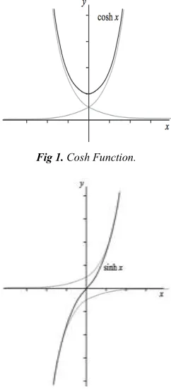
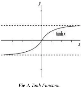
The hyperbolic functions have similar names to the trigonometric functions, but they are defined in terms of the exponential function. The three main types of hyperbolic functions, and the sketch of their graphs are giving below.

Fig 1. Cosh Function

Fig 2. Sinh Function

Methods

, &+ , (1) is the response variable, is the independent variable, B is the vector of the parameters _- to is a random error term , ( is the number of unknown parameters, is the number of

-’s are found by minimizing ) function

! , &+. (2) Under the assumption that the are normal and independent with mean zero and common variable / . Since are fixed observations, the sum of squares residual is a function of B, these normal equations take the form of

&+0 12 34,5+

167 0 (3)

. When the model is nonlinear in the parameters so are the normal equations consequently, for the nonlinear model consider the table 2, it is impossible to obtain the closed solution of the least squares estimate of the normal equations describe in Eq (3). Hence an iterative method must be employed to minimize (Draper and Smith 1981, Ratkowsky 1983,

, Seber & Wild 1989, Fekedulegn 1996). The hyperbolic functions have similar names to the

functions, but they are defined in terms of the exponential function. The three main types of hyperbolic

their graphs are giving below.

Cosh Function.

Pure and Applied Mathematics Journal 2014; 3(5): 99-104 101

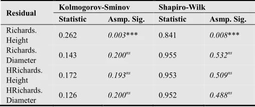
Fig 3. Tanh Function.

According to Oyamakin et al. (2013), the hyperbolic sine function and its inverse provide an alternative method for evaluating;

9 1

√1 + ; <; If we make the substitution, then;

=1 + ; = =1 + ) ℎ ?) = =@A)ℎ ?) = cosh ?) Where the second equality follows from the identity cosh2(u) − sinh2(u) = 1 and the last equality from the fact that cosh(u) > 0 for all u. Hence;

9 1

√1 + ; <; = 9

cosh ?) cosh ?) <? = 9 <? = ? + @ = ) ℎG _{;) + @}

The following proposition is a consequence of the integral above i.e.

<

<; ) ℎG ;) =_{√1 + ;}1

Also, using the substitution x = tan (u), −H< ? <H , that

9 1

√1 + ; <; = JAK L; + =1 + ; L + @

Since two anti-derivatives of a function can differ at most by a constant, there must exist a constant k such that

) ℎG _{;) = JAK L; + =1 + ; L + M}

for all x. Evaluating both sides of this equality at x = 0, we have

0 = ) ℎG _{0) = log 1) + M = M}

Thus k = 0 and

) ℎG _{;) = JAK L; + =1 + ; L}

for all x. Since the hyperbolic sine function is defined in terms of the exponential function, we should not find it

surprising that the inverse hyperbolic sine function may be expressed in terms of the natural logarithm function.

3. Hyperbolastic Richards’ Growth

Model (HRGM)

= 1 − + P

√1 +

= − + P

√1 + Multiply through by A AQ R ;

= − ) + P

√1 + Separating variables give;

− ) = +_{√1 +}P <

− T = +_{√1 +}P <

Divide LHS by T to have;

G G

− G < = +_{√1 +}P <

Using substitution method we have that; Let U = − G such that <U = −Q G G <

< =_−Q<U_{G G}

Substituting and integrating we have that;

−1_{Q J U = + PR @) ℎ ) + V}

−1_{Q J} − G _{) = + PR @) ℎ ) + V}

J − G ₎G _{= + PR @) ℎ ) + V}

− G ₎G _{= WX}YZT[\Y] "^ Z)

It therefore follows by little Algebra that;

=

1 + WXG [YZT[\Y] "^ Z)]₎

Therefore, we shall apply the two models below on Age-height and Age-Diameter of pines (pinus caribaea) growth;

(1) = _

` Ta*bc[defghdij4kl e)]_mnc+ o , and = _

(2) = _

` Ta*bdce_mnc+ o, and = _

` Ta*bdce_mcn+ o

4. Results and Discussion

4.1. Figures and Tables

Table 1. Summary of model selection criteria computed for the Proposed and Source models.

Models SSE N K R SQ MSE AIC

Source(ht) 29.431 17 4 90.90% 2.264 17.33019834

Proposed(ht) 15.579 17 5 95.20% 1.298 8.516078661

Source(dbh) 4.06 17 4 99.10% 0.312 -16.3445163

Proposed(dbh) 2.999 17 5 99.40% 0.25 -19.49388555

The table 1 below shows the estimated parameter for exponential and hyperbolic exponential growth model with their respective coefficient of determination (R2), MAE and MSE for age-height/age-diameter models.

Also, the predicted and observed height and diameter were plotted to show the relationship and how best the models predicted the observed data on height and diameter of pines. This is also shown in the figure below:

Fig 4. Observed Height against Predicted height (Richards growth model).

Fig 5. Observed Height against Predicted height (Hyperbolic Richards growth model)

Fig 6. Observed Diameter against Predicted diameter (Richards growth model).

Fig 7. Observed Diameter against Predicted diameter (Hyperbolic Richards growth model).

4.2. Testing for Independence of Errors (Run test) and Normality of Error (Shapiro-Wilk Test)

Table 2. Result of the test of independence of Residuals using Run Test.

Residual Test Value No of Runs Z Asymp. Sig.(2

tailed Richards.

Height -0.0218 5 -1.802 0.072

*

Richards.

Diameter 0.0041 7 -0.899 0.369

ns

HRichards.

Height -0.0047 6 -1.494 0.135

ns

HRichards.

Diameter -0.0012 8 -0.381 0.703

ns

* Significant at 10%, ** significant at 5%, *** significant at 99% and ns _not

significant.

Two assumptions made in the models are: Errors are independent

Errors are normally distributed.

These assumptions were verified by examining the residuals. If the fitted models are correct, residuals should exhibit tendencies that tend to confirm or at least should not exhibit a denial of the assumptions.

Hence, we tested the following hypotheses stated below; H0: Errors are independent (Using Runs Test)

Pure and Applied Mathematics Journal 2014; 3(5): 99-104 103

And

H0: Errors are normally distributed (Using Shapiro-Wilk test)

H1: Errors are not normally distributed

Let m be the number of pluses and n be the number of minuses in the series of residuals. The test is based on the number of runs(r), where a run is defined as a sequence of symbols of one kind separated by symbols of another kind. A good large sample approximation to the sampling distribution of the number of runs is the normal distribution with mean;

pXR =_{U + + 1}2U

and,

qR R @X / ) = 2U 2U − U − )_{U + ) U + − 1)}

Therefore, for large samples like ours the required test statistic is;

r = + ℎ − s)_/ ∼ u 0,1)

where,

ℎ = v 0.5, < s_{−0.5, > s} y

Also, the required test statistic for the test of normality (Shapiro-Wilk test) is given by;

z = Q Where;

= { R M){;"T G|− ;|)}

and,

Q = { ; − ;̅)

In the above, the parameter k takes the values; x(k) is the kth order statistic of the set of residuals and the values of coefficient a(k) for different values of n and k are given in the Shapiro-Wilk table. H0 is rejected at level α i.e. W is less than the tabulated value.

Table 3. Result of the test of normality of Residuals using K-S & S-W Tests.

Residual Kolmogorov-Sminov Shapiro-Wilk

Statistic Asmp. Sig. Statistic Asmp. Sig.

Richards.

Height 0.262 0.003*** 0.841 0.008***

Richards.

Diameter 0.143 0.200

ns _{0.955 0.532}ns

HRichards.

Height 0.172 0.193

ns _{0.953 0.509}ns

HRichards.

Diameter 0.126 0.200

ns _{0.952 0.488}ns

* Significant at 10%, ** significant at 5%, *** significant at 99% and ns _not

significant.

5. Conclusion

Finally, our proposed model showed a promising results and using the above discussed data sets, they fitted the data with smaller AIC, MSE, and higher prediction accuracy than its source model. We strongly believe that choosing a flexible and highly accurate predictive model such as ours can significantly improve the outcome of a study because the accuracy of a model is what determines its utility. Hence, we recommend usage of our proposed models to the scientific community and practitioners and urge comparison of them with classical models before decisions on model selection are made. We have succeeded in introducing a new growth model using the hyperbolic sine function. The mean function of top height and Dbh over age using the Hyperbolic Richards growth model predicted closely the observed values of top height and Diameter of Pines better than the source model.

References

[1] Bertalanffy, L. von. 1957. Quantitative laws in metabolism and growth. Quantitative Rev. Biology 32: 218-231.

[2] Brisbin IL: Growth curve analyses and their applications to the conservation and captive management of crocodilians. Proceedings of the Ninth Working Meeting of the Crocodile Specialist Group. SSCHUSN, Gland, Switzerland 1989. [3] Burkhart, H.E., and Strub, M.R. 1974. A model for simulation

or planted loblolly pine stands. In growth models for tree and stand simulation. Edited by J. Fries. Royal College of Forestry, Stockholm, Sweden. Pp. 128-135. Model of forest growth. J. Ecol. 60: 849–873.

[4] Curtis, R.O. (1967). Height-diameter and height-diameter-age equations for second-growth Douglas-fir. For. Sci. 13: 365-375. [5] Draper, N.R. and H. Smith, 1981. Applied Regression Analysis.

John Wiley and Sons, New York

[6] Fekedulegn, D. 1996. Theoretical nonlinear mathematical models in forest growth and yield modeling. Thesis, Dept. of Crop Science, Horticulture and Forestry, University College Dublin, Ireland. 200p.

[7] EK, A.R. ,E.T. Birdsall, and R.J.Spear (1984). As simple model for estimating total and merchantable tree heights. USDA. For. Serv. Res. Note NC-309.5p

[8] Kansal AR, Torquato S, Harsh GR, et al.: Simulated brain tumor growth dynamics using a three dimentional cellular automaton. J Theor Biol 2000, 203:367-82.Khamis, A. and Z. Ismail, 2004. Comparative study on nonlinear growth curve to tobacco leaf growth data. J. Agro, 3: 147 – 153.

[9] Kingland S: The refractory model: The logistic curve and history of population ecology. Quart Rev Biol 1982, 57: 29-51. [10] Marusic M, Bajzer Z, Vuk-Pavlovic S, et al.: Tumor growth in vivo and as multicellular spheroids compared by mathematical models. Bull Math Biol 1994, 56:617-31.

[12] Myers, R.H. 1996. Classical and modern regression with applications. Duxubury Press, Boston. 359p.

[13] Nelder, J.A. 1961. The fitting of a generalization of the logistic curve. Biometrics 17: 89-110.

[14] Olea N, Villalobos M, Nunez MI, et al.: Evaluation of the growth rate of MCF-7 breast cancer multicellular spheroids using three mathematical models. Cell Prolif 1994, 27:213-23. [15] Oyamakin S. O., Chukwu A. U., (2014): On the Hyperbolic Exponential Growth Model in Height/Diameter Growth of PINES (Pinus caribaea), International Journal of Statistics and Applications, Vol. 4 No. 2, 2014, pp. 96-101. doi: 10.5923/j.statistics.20140402.03.

[16] Oyamakin, S. O.; Chukwu, U. A.; and Bamiduro, T. A. (2013) "On Comparison of Exponential and Hyperbolic Exponential

Growth Models in Height/Diameter Increment of PINES (Pinus caribaea)," Journal of Modern Applied Statistical Methods: Vol. 12: Iss. 2, Article 24. Pp 381 – 404.

[17] Philip, M.S., 1994. Measuring trees and forests. 2nd Edition CAB International, Wallingford, UK

[18] Ratkowskay, D.A., 1983. Nonlinear Regression modeling. Marcel Dekker, New York. 276p

[19] Seber, G. A. F. and C. J. Wild, 1989. Nonlinear Regression. John Wiley and Sons: NY

[20] Vanclay, J.K. 1994. Modeling forest growth and yield. CAB International, Wallingford, UK. 380p.