On the Effectiveness of Laplacian Normalization for Graph Semi-supervised Learning

(1)

On the Effectiveness of Laplacian Normalization for Graph

Semi-supervised Learning

Rie Johnson [email protected]

IBM T.J. Watson Research Center Hawthorne, NY 10532, USA

Tong Zhang [email protected]

Yahoo! Inc.

New York City, NY 10011, USA

Editor: Charles Elkan

Abstract

This paper investigates the effect of Laplacian normalization in graph-based semi-supervised learn-ing. To this end, we consider multi-class transductive learning on graphs with Laplacian regular-ization. Generalization bounds are derived using geometric properties of the graph. Specifically, by introducing a definition of graph cut from learning theory, we obtain generalization bounds that depend on the Laplacian regularizer. We then use this analysis to better understand the role of graph Laplacian matrix normalization. Under assumptions that the cut is small, we derive near-optimal normalization factors by approximately minimizing the generalization bounds. The analysis reveals the limitations of the standard degree-based normalization method in that the resulting normaliza-tion factors can vary significantly within each connected component with the same class label, which may cause inferior generalization performance. Our theory also suggests a remedy that does not suffer from this problem. Experiments confirm the superiority of the normalization scheme motivated by learning theory on artificial and real-world data sets.

Keywords: transductive learning, graph learning, Laplacian regularization, normalization of graph Laplacian

1. Introduction

Graph-based methods, such as spectral embedding, spectral clustering, and semi-supervised learn-ing, have drawn much attention in the machine learning community. While various ideas have been proposed based on different intuitions, only recently have there been theoretical studies trying to understand why these methods work.

(2)

universally acceptable criterion, it is difficult to argue that one cut definition is better than another just based on heuristics. If a universally agreeable standard does exist, then one should focus on that criterion instead of an artificially defined cut problem.

For example, in the context of spectral clustering, there are two well-known types of graph cut, the ratio cut (Hagen and Kahng, 1992) and the normalized cut (Shi and Malik, 2000). Approximate optimization of the ratio cut leads to eigenvector computation of the unnormalized graph Laplacian matrix (which we will define later), and that of the normalized cut involves the normalized graph Laplacian matrix (normalized using node degrees). Although a number of empirical studies indicate that the normalized cut often leads to better clustering results, there isn’t any direct theoretical proof except for some implicit evidence. As another example, the definition of graph Laplacian in the spectral graph theory in Chung (1998) is normalized, but that is for graph theoretical reasons instead of statistical reasons. Specifically, the normalized Laplacian allows easier translation of results from differential geometry, and it also allows consistent relations with conductance on Markov chains. The compatibility of continuous Laplacian on manifold and normalized graph Laplacian was also noted by von Luxburg et al. (2005) from a different perspective. Similarly, some analysis of spectral clustering employs normalized cut (Meil˘a et al., 2005, for example) as that makes derivation easier. These can be regarded as implicit evidence for preferring the normalized Laplacian over the unnor-malized Laplacian. However, it has not been directly proved that such degree-based normalization (corresponding to normalized cut) should improve performance.

In order to understand this issue better, we take a different approach in this paper. Observe that for spectral clustering applications, there are often pre-defined (but unknown) clusters (classes). In this setting, the goal is to find such classes either using unsupervised or semi-supervised methods. Therefore for such problems, a universally agreeable standard is to find clusters that overlap sig-nificantly with the underlying class labels. That is, instead of using any artificially defined cut, we should design an algorithm to minimize the classification error. This is the criterion we focus on in this paper. We will see that normalization comes naturally into the generalization analysis we develop. By optimizing the corresponding generalization bounds, we seek to obtain a better understanding of the effect of Laplacian normalization.

(3)

and the kernel fully determines the outcome of the k-means algorithm. Therefore this approach can also be viewed as designing a kernel optimal for clustering.

Closely related to clustering, one may also consider kernel design methods in semi-supervised learning using a discriminative method such as SVM (e.g., Lanckriet et al., 2004). In this setting, the change of the distance metric becomes a change of the underlying kernel. If the kernel is induced from a graph, then one may formulate semi-supervised learning directly on the graph; for example, see Belkin and Niyogi (2004), Szummer and Jaakkola (2002), Zhou et al. (2004) and Zhu et al. (2003). In these studies, the kernel is induced from the adjacency matrix W whose(i,j)-entry is the weight of edge(i,j). W is often normalized by D−1/2WD−1/2as in Chung (1998), Shi and Malik (2000), Ng et al. (2002), Zhou et al. (2004), where D is a diagonal matrix whose(j,j)-entry is the degree of the j-th node, but sometimes not (Belkin and Niyogi, 2004, Zhu et al., 2003). Although such normalization can significantly affect the performance, the issue has not been carefully studied from the learning theory perspective. The relationship of kernel design and graph learning was investigated in Zhang and Ando (2006), where it was argued that quadratic regularization-based graph learning can be regarded as kernel design in the spectral domain. That is, one keeps the kernel eigenvectors and modifies the corresponding eigenvalues. Moreover if input data are corrupted with noise, then such spectral kernel design can help to improve classification performance. However, the analysis does not explain why normalization of the adjacency matrix W is useful for practical purposes.

Our goals here are twofold. First we present a model for transductive learning on graphs and develop a margin analysis for multi-class graph learning. We then analyze graph learning using graph properties such as graph-cut and a concept we call pure subgraph. The analysis naturally employs quantities formalizing the standard graph-learning assumption that well connected nodes are likely to have the same label. Second, we use this analysis to obtain a better understanding of normalizing the Laplacian matrix (D₋W) in graph semi-supervised learning. As mentioned

above, normalization has been commonly practiced and appears to be useful, but there hasn’t been any solid theoretical justification on why it should be useful. Our analysis addresses this issue from a learning theoretical point of view, and reveals a limitation of the standard degree-based normalization scheme. We then propose a remedy based on the learning theory results and use experiments to demonstrate that the remedy leads to improved classification performance.

This paper expands on our preliminary results reported in Ando and Zhang (2007).

2. Transductive Learning Model

We consider the following multi-category transductive learning model defined on a graph. Let

V =_{v1, . . . ,vm} be a set of m nodes, and let

Y

be a set of K possible output values. Assume

that each node vj is associated with an output value yj∈

Y

, which we are interested in predicting.

In order to do so, we randomly draw a set of n indices Zn={ji : 1≤i≤n} from {1, . . . ,m}

uniformly and without replacement. We manually label the n nodes vji with labels yji∈

Y

, and then automatically label the remaining m₋n nodes. The goal is to estimate the labels on the remaining m₋n nodes as accurately as possible.

In this paper, we shall assume that the labels y= [y1, . . . ,ym]are deterministic. However, the

analysis can also be applied if we have random labels. In the transductive learning setting consid-ered in this paper, we may assume that we are given a single random draw y= [y1, . . . ,ym], which

(4)

subset of labels. This formulation is more appropriate for problems such as classification on graphs considered here.

In modern machine learning, instead of estimating the labels yj directly, yj is often encoded

into a vector in RK, so that the problem becomes that of generating an estimation vector fj =

[fj,1, . . . ,fj,K]∈RK, which can then be used to recover the label yj. In multi-category

classifica-tion with K classes

Y

=_{1, . . . ,K_}, we encode each yj=k∈

Y

as ek∈RK, where ekis a vector of

zero entries except for the k-th entry being one. Given a function fj= [fj,1, . . . ,fj,K]∈RK (which is

intended to approximate eyj), we decode the corresponding label estimation ˆyjas:

ˆ

yj=yˆ(fj) =arg max k

fj,k: k=1, . . . ,K .

If the true label is yj, then the corresponding classification error is:

err(fj,yj) =I(yˆ(fj)6=yj),

where we use I(_·)to denote the set indicator function.

In order to estimate the concatenated vector f= [fj] = [fj,k]∈RmKfrom only a subset of labeled

nodes, we have to impose restrictions on possible values of f. In this paper, we consider restrictions defined through a quadratic regularizer of the following form:

fTQKf=

K

∑

k=1

fT_·_,_kK−1f_·,k,

where K_∈Rm×m is a positive definite kernel matrix and f_·,k = [f1,k, . . . ,fm,k]∈Rm. That is, the

predictive vector for each class k is regularized separately. We assume that the kernel matrix K is full-rank. We will consider the kernel matrix induced by the graph Laplacian, which we shall define later in the paper. Note that we use the bold symbol K to denote the kernel matrix and the regular capitalized K to denote the number of classes.

Given a vector f_∈RmK, the accuracy of its component fj= [fj,1, . . . ,fj,K]∈RK is measured by

a loss functionφ(fj,yj). Our learning method attempts to minimize the empirical risk on the set Zn

of n labeled training nodes, subject to fTQKf being small:

ˆf(Zn) =arg min

f∈RmK

"

1

n _j

∑

_∈_Z

n

φ(fj,yj) +λfTQKf

#

. (1)

whereλ>0 is an appropriately chosen regularization parameter.

In this paper, we focus on a special class of loss functions of the formφ(fj,yj) =∑Kk=1φ0(fj,k,δk,yj), whereδa,bis the delta function defined as:δa,b=1 when a=b andδa,b=0 otherwise. In addition,

we introduce the following assumption for convenience.

Assumption 1 Let φ(fj,yj) =∑kK=1φ0(fj,k,δk,yj) in (1), where fj = [fj,1, . . . ,fj,K]∈R

K_{. Assume}

that there exist positive constants a, b, and c such that

• φ0(x,y)is non-negative and convex in x.

(5)

• c=inf{x :φ0(x,1)≤a} −sup{x :φ0(x,0)≤a}.

The formulation presented here corresponds to the one-versus-all method for multi-category classi-fication, and standard binary loss functions such as least squares, logistic regression, and SVMs can be used. For the SVM loss functionφ0(x,y) =max(0,1−(2x−1)(2y−1)), we may take a=0.5, b=2, and c=0.5. For the least squares function φ0(x,y) = (x−y)2, we may choose a=1/16, b=0.5, c=0.5.

We are interested in the generalization behavior of (1) compared to a properly defined optimal regularized risk. This type of inequality is often referred to as “oracle inequality” in the learning the-ory literature and is particularly useful for analyzing the quality of the underlying learning method. The following theorem gives an oracle inequality, and its proof can be found in Appendix A.

Theorem 1 Consider (1) with loss functionφsatisfying Assumption 1. Then_∀p>0, the expected

generalization error of the learning method (1) over the training samples Zn, uniformly drawn without replacement from graph nodes_{1, . . . ,m_}, can be bounded by:

EZn 1

m₋n

∑

j∈_Z¯_n

err(ˆfj(Zn),yj)≤

1

af∈infRmK

"

1

m m

∑

j=1

φ(fj,yj) +λfTQKf

#

+

btrp(K)

λnc

p

,

where ¯Zn={1, . . . ,m} −Zn,

trp(K) =

1

m m

∑

j=1

Kp_j_,_j

!1/p

,

and Kj,jdenotes the j-th diagonal entry of matrix K.

If we take p=1 in Theorem 1, then the bound depends on the trace of matrix K: tr(K) =

mtr1(K). The trace of a kernel matrix has been employed in a number of previous studies to char-acterize generalization ability of kernel methods. The generalized quantity in Theorem 1 with p₆=1 has non-trivial consequences which we will investigate in the paper.

Although we consider a specific form of loss function in this paper, one can obtain similar bounds with other forms of loss functions such asφ(fj,yj) =supk6=yjφ0(fj,yj−fj,k). What is im-portant in our analysis are the two quantities fTQKf and trp(K) that determine the generalization

performance. We will focus on the interpretation of these quantities.

3. Margin and Graph Cut

Consider an undirected graph G= (V,E)defined on the nodes V =_{vj: j=1, . . . ,m}, with edges E_{⊂ {}1, . . . ,m_{} × {}1, . . . ,m_}, and weights wj,j0≥0 associated with edges(j,j0)∈E. For simplicity, we assume that(j,j)_∈/E and wj,j0=0 when(j,j0)∈/E. Let deg_j(G) =∑m_j0₌₁wj,j0 be the degree of node j of graph G. We consider the following definition of normalized Laplacian.

Definition 2 Consider a graph G= (V,E) of m nodes with weights wj,j0 ( j,j0=1, . . . ,m). The

unnormalized Laplacian matrix

L

(G)_∈Rm×m_{is defined as:}

L

j,j0(G) =−wj,j0 if j6= j0; deg_j(G)

otherwise. Given m scaling factors Sj ( j=1, . . . ,m), let S=diag({Sj}). The S-normalized Lapla-cian matrix is defined as:

L

S(G) =S−1/2

L

(G)S−1/2.The corresponding regularization is based

on:

fT_·_,_k

L

S(G)f·,k=

1 2

m

∑

j,j0₌₁

wj,j0 _pfj,k

Sj− fj0_,_k

p

Sj0

!2

(6)

A common choice of S is S=I, corresponding to regularizing with the unnormalized Laplacian

L

. The idea is natural: we assume that the predictive values fj,k and fj0_,_k should be close when (j,j0)_∈E with a strong link. Another common choice is to normalize by Sj =degj(G), as in

Ng et al. (2002), Shi and Malik (2000), Zhou et al. (2004) and Chung (1998), which we refer to as degree-based normalization. At first sight, the need for normalization is not immediately clear. However, as we will show later, normalization using appropriate scaling factors can improve performance.

3.1 Generalization Analysis Using Graph-Cut

We will adapt Theorem 1 in Section 2 to analyze graph learning using graph properties such as graph-cut. We now introduce a learning theoretical definition of S-normalized graph cut as follows.

Definition 3 Given label y=_{yj}j=1,...,m on V , we define the cut for the S-normalized Laplacian

L

Sin Definition 2 as:

cut(

L

S,y) =

∑

j,j0_:y_j₆₌_y_j0

wj,j0 2

1

Sj

+ 1

Sj0

+

∑

j,j0_:y_j₌_y_j0

wj,j0 2

1

p

Sj

−p1

Sj0

!2

.

Note that unlike typical graph-theoretical definitions of graph-cut in the literature, the learning theoretical definition of cut not only penalizes a normalized version of between-class edge weights, but also penalizes within-class edge weights when such an edge connects two nodes with different scaling factors. This difference has important consequences, which we will investigate later in the paper. For unnormalized Laplacian, the second term on the right hand side of Definition 3 vanishes, which means that it only penalizes weights corresponding to edges connecting nodes with different labels. In this case, the learning theoretical definition corresponds to the graph-theoretical definition:

cut(

L

,y) =∑j,j0_:y_j₆₌_y_j0w_j_,_j0.

It is worth noting that in our framework, cut is used to indicate the absolute amount of pertur-bation from the idealized case with zero-cut. In spectral clustering, the absolute cut is often scaled and the resulting quantity is used as a quality measure for the clusters. In comparison, our quality measure is always to minimize the classification error. In particular, the unnormalized Laplacian is used in spectral clustering to approximately minimize the ratio cut =∑_j_∈_A_,_j0_∈_Bwj,j0/(|A| · |B|) (Hagen and Kahng, 1992) instead of∑j_∈A,j0_∈_Bw_j_,_j0. The scaling in the ratio cut (when K=2) corre-sponds to the normalization of a specific encoding of the target vectors (f_·,k∈Rmwhich encodes the

(7)

Using the learning theoretical graph-cut definition, we can obtain a generalization result for the estimator in (1) with K defined as follows:

K−1=αS−1+

L

S(G) =S−1/2(αI+

L

(G))S−1/2, (2) where I is the identity matrix. Note that α>0 is a tuning parameter to ensure that K is strictly positive definite. As we will see later, this parameter is important. The corresponding regularization condition is

fTQKf=

K

∑

k=1



α

m

∑

j=1

f_k2_,_j Sj

+1

2

m

∑

j,j0₌₁

fj,k

p

Sj − fj0_,_k

p

Sj0

!2

wj,j0



.

Another possibility is to let K−1=αI+

L

S(G). The conclusions, which we will not include in this paper, are similar to that of (2).

For simplicity, we state the generalization bound based on Theorem 1 with optimal λ. Note that in applications, λ is usually tuned through cross validation. Therefore assuming optimal λ will simplify the bound so that we can focus on the more essential characteristics of generalization performance. The following assumption is used to simplify the bound

Assumption 2 Consider (1) with regularization condition (2), loss functionφsatisfying Assump-tion 1, and assume thatφ0(0,0) =φ0(1,1) =0.

It is easy to check that the conditions on the loss function in Assumption 2 hold for the least squares method (which we focus on in this paper) as well as other standard loss functions such as SVM.

Theorem 4 Consider (1) such that Assumption 2 is satisfied. Then_∀p>0, there exists a sample

in-dependent regularization parameterλin (1) such that the expected generalization error is bounded by:

EZn 1

m−n_j

∑

∈_Z¯_n

err(ˆfj(Zn),yj)≤

Cp(a,b,c)

np/(p+1) (αs+cut(

L

S,y))

p/(p+1)_tr

p(K)p/(p+1),

Cp(a,b,c) =(b/ac)p/(p+1)(p1/(p+1)+p−p/(p+1)), (3) where s=∑m_j₌₁S−_j1.

Proof Let fj,k=δyj,k. It can be easily verified that

1

m m

∑

j=1

φ(fj,yj) +λfTQKf=λ(αs+cut(

L

S,y)).

Now, using this expression in Theorem 1, and then optimizing overλ, we obtain the desired in-equality.

Note that with the least squares loss, we can take b/ac=16 in Theorem 1. With a fixed p, the generalization error decreases at the rate O(n−p/(p+1)₎_{when the sample size n increases. This rate of} convergence is faster when p increases. However in general, trp(K)is an increasing function of p.

(8)

we will consider later in the paper), one may prefer a smaller p in order to optimize the bound. An analysis will be provided in the next section. The bound also suggests that if we normalize K so that its diagonal entries Kj,j become a constant, then trp(K)is independent of p, and thus a larger p can be used in the bound. This motivates the idea of normalizing the diagonals of K, which

we will further investigate later in the paper. The generalization bound in Theorem 4 is closely related to the margin analysis for binary linear classification. Specifically, the right hand side can be viewed as a margin-like-quantity associated with the target function fj,k=δyj,kthat separates the data. Here it is related to the concept of graph cut. Our goal is to better understand the quantity (αs+cut(

L

S,y))p/(p+1)trp(K)p/(p+1)using graph properties, which gives better understanding of

graph based learning.

In the following, we will give example applications of Theorem 4. They illustrate that theoreti-cally it is important to tune the parameterαto achieve good performance, which is also empirically observed in our experiments.

3.2 Zero-cut and Geometric Margin Separation

We consider an application of Theorem 4 for the unnormalized Laplacian under the zero-cut as-sumption that each connected component of the graph has a single label. With this asas-sumption, the task is simply to estimate what label each connected component has.

Theorem 5 Consider (1) such that Assumption 2 is satisfied and the regularization condition is K−1=αI+

L

. Assume that cut(

L

,y) =0, and the graph has q connected components of sizes

m1≤ ··· ≤mq(∑`m`=m). For all p>0, letα→0, and with optimalλ, we have the generalization bound

EZn 1

m₋n_j

∑

∈Z¯n

err(ˆfj,yj)≤

Cp(a,b,c) np/(p+1)

q

∑

`=1

(m/m`)p−1

!1/(p+1)

+O(α),

where Cpis defined in (3). In particular, we have

EZn 1

m₋n

∑

j∈_Z¯_n

err(ˆfj,yj)≤min

"

2

r

b ac·

q n,

b ac·

m nm1

#

+O(α).

Proof Since the graph has q connected components,

L

has q eigenvectors v`(`=1, . . . ,q)

associ-ated with zero-eigenvalues, where each eigenvector v`is the indicator function of the`-th connected

component in the graph, that is, the j-th entry of vector v` is 1 if j belongs to the`-th connected

component and 0 otherwise. It is not hard to check that as α_→0, αK_→∑q_`₌₁_m1 `v`v

T

` +O(α).

Therefore αtrp(K)→m−1/p(∑q_`₌₁m1_`−p)1/p. Now, we can use Theorem 4 to obtain the first

in-equality. The second inequality is obtained by setting p=1 and by letting p_→∞on the right hand side.

Under the zero-cut assumption, the generalization performance can be bounded as O(p

(9)

q. This implies that we will achieve better convergence at the O(1/n) level if the sizes of the components are balanced. If the component sizes are significantly different, the convergence may behave like O(p

q/n).

We discuss a concrete example in which Theorem 5 is applicable. Assume that each node vj is

associated with a data point xj that belongs to the d-dimensional unit ball B={x∈Rd:kxk2≤1}.

We form a graph by connecting all nodes vj to their nearest neighbors. In particular, we may

consider an ε-ball centered at each vj: Bj(ε) ={x :kx−xjk2 ≤ε}. We then form a graph by

connecting each j with all points within the ball Bj(ε)and with unit weights.

We say that the data points are separable with geometric marginγif for each node vj the ball Bj(γ) only contains points in class yj. Now assume we use a ball of size ε≤γ. In this case, cut(

L

,y) =0, and there is a constant q_≤ε−d such that the graph has at most q connected compo-nents, and we have:

EZn 1

m₋n

∑

j∈_Z¯_n

err(ˆfj,yj)≤2

r

b ac·

q

n+O(α).

This bound does not depend on marginγbut depends only on q, the number of connected compo-nents. So even if the marginγis small, the bound can still be good as long as q is small. This result can be used to understand why graph based semi-supervised learning may work better than stan-dard kernel learning. In fact, it is not possible to derive similar generalization bounds for supervised learning because one needs unlabeled data (in addition to labeled data) to define such connected components. This means that graph semi-supervised learning can take advantage of the new quan-tity q to characterize its generalization performance, and this quanquan-tity cannot be used by standard supervised learning.

Note that we have assumed a very specific generative model for the data. In particular, if the data are generated in a way such that the number of connected components q is small, and each connected component belongs to a single class, then graph based semi-supervised learning can work better than supervised kernel learning. If this assumption does not hold (at least approximately), then graph based learning methods may fail. However, for many practical applications, the geometric margin separation assumption does appear quite reasonable. Therefore for such problems, graph based semi-supervised learning, which can take advantage of the underlying data generation model, may become helpful.

This section only considers a special case where the graph has q connected components. In this particular situation, the learning method (1) and the analysis provided here may not be optimal. The best method is just to identify each connected component to be a cluster and then determine its label by looking at one point of the cluster. However, this idea won’t generalize to graphs with components that are weakly connected. In comparison, our analysis can easily generalize to that situation, as we shall investigate in the next section.

3.3 Non-Zero Cut and Pure Components

It is often too restrictive to assume that each connected component has only one label (that is, the cut is zero). In this section, we show that similar bounds can be obtained when this data generation assumption is relaxed. We are still interested in giving a characterization of the performance of (1) in terms of properties of the graph and introduce the following definition.

(10)

G0=_∪q_`₌₁G`of G divides V into q disjoint sets V =_∪q_`₌₁V`such that each subgraph G`= (V`,E`)

is a pure component. Denote byλi(G`) =λi(

L

(G`))the i-th smallest eigenvalue of

L

(G`).

For instance, if we remove all edges of G that connect nodes with different labels, then the resulting subgraph is a pure subgraph (though it may not be the only one). For each pure component

G`, its first eigenvalueλ1(G`) is always zero. The second eigenvalue λ2(G`)>0 because G` is

connected. Thisλ2(G`)can be regarded as a measurement of how well G`is connected. We use it

together with graph cut to derive a generalization bound. The proof is given in Appendix B.

Theorem 7 Consider (1) such that Assumption 2 is satisfied. Let G0=_∪q_`₌₁G`(G`= (V`,E`)) be a pure subgraph of G. For all p_≥1, there exist sample-independent regularization parameterλand a fixed tuning parameterα, such that

EZn 1

m₋n _j

∑

∈Z¯n

err(ˆfj,yj)

≤Cp(a,b,c)

np/(p+1)



s1/2

q

∑

`=1

s`(p)/m m_`p

!1/2p

+cut(

L

S,y)1/2

q

∑

`=1

s`(p)/m λ2(G`)p

!1/2p



2p/(p+1) ,

where Cpis defined in (3), m`=|V`|, s=∑mj=1S−j1, and s`(p) =∑j∈V`S p j.

Theorem 7 is a natural generalization of Theorem 5 when p_≥1. It quantitatively illustrates the importance of analyzing graph learning using a partition of the original graph into well-connected pure components. The second eigenvalue λ2(Gi) measures how well-connected Gi is. A more

intuitive quantity that measures the connectedness of graph G= (V,E)is the isoperimetric number

hGdefined as

hG= inf S⊂V_j

∑

∈S,j0_∈_V₋_S

wj,j0/min(|S|,|V−S|).

It is well-known thatλ2(Gi)≥h2Gi/(2 maxjdegj(Gi))(Chung, 1998). The isoperimetric number of a graph is large when the nodes are well-connected everywhere. In particular, if deg_j(G)is of the order_|V_|, and wi,j=1 when(i,j)∈E, then for a well-connected graph,∑j_∈S,j0_∈_V₋_Sw_j_,_j0 is of the order _|S_||V₋S_|, and hG=O(|V|). Let G0 be a well-behaved pure-subgraph of G, such that each

pure component G`of G0is well-connected in the above sense. We thus have the condition

λ2(G`)/m`≥u(G0)

for some constant u(G0) that does not depend on the size of the pure components (but only how well-connected each pure component is). Under this condition, we may replace∑q_`₌₁m`λ2(G`)−p

by u(G0)−p_∑q `=1m

1₋p

` in Theorem 7 and obtain a simplified bound:

EZn 1

m₋n _j

∑

∈Z¯n

err(ˆfj,yj)≤

Cp(a,b,c) np/(p+1)

q

∑

`=1

s`(p)/m

(m`/m)p

!1/(p+1) _r

s

m+

s

cut(

L

S,y)

u(G0₎_m

!2p/(p+1)

(11)

where we define u(G0) =min`(λ2(G`)/m`). We consider two special cases: p=1 and p→∞:

EZn 1

m₋n_j

∑

∈Z¯n

err(ˆfj,yj)≤2

s

b ac·

∑q

`=1(s`(1)/m`) n

r

s

m+

s

cut(

L

S,y)

u(G0₎_m

!

, (4)

EZn 1

m₋n_j

∑

∈_Z¯_n

err(ˆfj,yj)≤ b ac·

max`maxj∈V`(Sj/m`) n

√

s+

s

cut(

L

S,y)

u(G0)

!2

. (5)

These bounds are generalizations of those in Theorem 5. Suppose that we take S=I. Then the

number of pure components q affects the O(1/√n)convergence rate in (4) as∑q_`₌₁s`(1)/m`=q. If

the sizes of the components are balanced, we can achieve better convergence at the O(1/n)level as in (5); otherwise, the convergence may behave like O(pq/n). This observation motivates a scaling matrix S that compensates for the unbalanced pure component sizes, which we will investigate next.

3.4 Optimal Normalization for Near-zero-cut Partition

As discussed in the introduction, the common practice of the normalization of the adjacency matrix (W) or the graph Laplacian (D₋W) is based on degrees, which corresponds to setting S=D.

Although such normalization may significantly affect the performance, to our knowledge, there is no learning theory analysis on the effect of normalization. The purpose of this section is to fill this gap using the theoretical tools developed earlier. We shall focus on a near ideal situation to gain intuition.

Consider a pure subgraph G0=_∪q_`₌₁G`(G`= (V`,E`)) of G. If scaling factors Sj are

approx-imately constant within each pure component, then using the Laplacian in Definition 2, we have a small regularization penalty for the edges within a pure component and between the nodes that have close output values (i.e., fj,k ≈ fj0_,_k). Therefore, in the following we focus on finding the op-timal scaling matrix S such that Sjis constant within each pure component V`, and assume that S is

quantified by q numbers[s`¯]`=1,...,q, such that Sj=s`¯ when j∈V`.

Consider the following quantity:

cut(G0,y) =

∑

j,j0_:y_j₆₌_y j0

wj,j0+

∑

`6=`0_j_∈_V_`

∑

_,_j0_∈_V

`0 wj,j0

2 .

It is easy to check that

cut(

L

S,y)≤cut(G0,y)/min

` s¯`.

Assume that weights are small between pure components, and therefore, cut(G0,y)is small. With the O(1/n)convergence rate, we obtain from (5) that

1

m₋n _j

∑

∈Z¯n

max`(s`/m`¯ ) n

s _q

∑

`=1

m`/s`¯ +

s

cut(G0,y)

u(G0)min`s¯`

!2

.

If cut(G0,y)is small, then the dominating term on the right hand side is

max`(s`/m`¯ ) n

q

∑

`=1

m`

¯

(12)

which can be optimized with the choice ¯s`=m`, and the resulting bound becomes:

1

m₋n_j

∑

∈Z¯n

1

n

√_q₊s cut(G0,y)

u(G0₎_min_`_m_`

!2

.

That is, if cut(G0,y)is small, then we can choose scaling factor ¯s`∝m`for each pure component`

so that the generalization performance is approximately(ac)−1_b_·_{q/n, which is of the order O}₍₁_/n₎_.

The analysis provided here not only proves the importance of normalization under the learn-ing theoretical framework, but also suggests that the good normalization factor for each node j is approximately the size of the well-connected pure component that contains node j (assuming that nodes belonging to different pure components are only weakly connected). Our analysis focused on the case that the scaling factors are a constant within each pure component. This condition is quite natural if we look at the normalized Laplacian regularization condition in Definition 2, where

fj,k/

p

Sj should be similar to fj0_,_k/pS_j0 when w_j_,_j0 is large. If j and j0belongs to the same class, then fj,k should be similar to fj0_,_k. Therefore for such a pair (j,j0), we want to have S_j ≈S_j0 if

wj,j0 is large. Note that this requirement is not enforced by the standard degree-based normalization method Sj=degj(G)because a well-connected pure component may contain nodes with quite

dif-ferent degrees. The assumption is satisfied under a simplified “box model”, which is related to the models used by some previous researchers to derive the standard normalization method (e.g., Shi and Malik, 2000). In this model, a pure component is completely connected, and each node connects to all other nodes and itself with edge weight wj,j0 =1. The degree is thus deg_j(G_`) =|V_`|=m_`, which gives the optimal scaling in our analysis.

In general, the box model may not be a good approximation for practical problems. A more realistic approximation, which we call core-satellite model, will be introduced in the experimental section. For such a model, the degree-based normalization can fail because the deg_j(G`) within

each pure component G` is not approximately constant, and it may not be proportional to m`. In

general, this approximation using degrees causes Sj to potentially vary significantly within a pure

component because each Sjis only determined by its immediate neighbors.

Our analysis suggests that it is necessary to modify the degree-based scaling method Sj =

deg_j(G)so that the scaling factor is approximately a constant within each pure component, which should be proportional to m`. Our remedy is to look for connected components at a larger distance

scale. Although there could be various methods to achieve this effect, we shall focus on a specific method motivated by the proofs of Theorem 5 and Theorem 7. Let ¯K= (αI+

L

)−1 _{be the}

ker-nel matrix corresponding to the unnormalized Laplacian. Using the terminology in the proofs, we observe that for smallα:

α_K¯ ₌

q

∑

`=1

v`vT`/m`+O(1),

and thus ¯Kj,j ∝m−_`1for each j∈V`. Therefore with smallα, the scaling factor Sj=1/K¯ j,j is near

optimal for all j. For α>0, the effect of this scaling factor is essentially equivalent to looking for connected components at a scale of at most O(1/α)number of nodes. We call this method of normalization K-scaling in this paper. It is equivalent to a normalization of the kernel matrix K, so that each Kj,j =1. Although this method coincides with a common practice in standard kernel

(13)

method in the graph learning setting before. In fact, without learning theoretical results developed in this paper, it is not obvious that this method should work better than the more standard degree-based normalization method. In our framework, the main advantage of K-scaling (compared to the standard degree-scaling, which we call L-scaling) is twofold:

• The resulting Sjdoes not vary significantly within a well-connected pure component.

• The resulting scaling is approximately m`(at a scale of 1/α), which is predicted by our theory

to be desirable.1

The superiority of this method will be demonstrated in our experiments. The main drawback of this method is the computational cost of directly inverting (αI+

L

). For large scale problems, approximation methods are required.

3.5 Dimension Reduction

Normalization and dimension reduction have been commonly used in spectral clustering such as Ng et al. (2002) and Shi and Malik (2000). For semi-supervised learning, dimension reduction (without normalization) is known to improve performance (Belkin and Niyogi, 2004, Zhang and Ando, 2006) while the degree-based normalization (without dimension reduction) has also been explored (Zhou et al., 2004). In this section, we present a brief high-level argument that an appropriate combination of normalization and dimension reduction (as commonly used in spectral clustering) can improve classification performance. Detailed analysis can be found in Appendix C.

Let us first introduce dimension reduction with normalized Laplacian

L

S(G). Denote by Pr_S(G) the projection operator onto the eigenspace ofαS−1+

L

S(G)corresponding to the r smallest eigen-values. Now, we may define the following regularizer on the reduced subspace:

fT_·_,_kK−1f_·,k=

(

fT

·,kK−01f·,k if PSr(G)f·,k=f·,k,

+∞ otherwise. (6)

The benefit of dimension reduction in graph learning has been investigated in Zhang and Ando (2006), under the spectral kernel design framework. The idea is to modify the kernel eigenvalues so that the target spectral coefficient matches the kernel coefficients. Note that the normalization issue, which will change the eigenvectors and their ordering, wasn’t investigated there. However, with a fixed scaling matrix S, the reasoning given in Zhang and Ando (2006) can also be applied here. It was shown there that if noise is added into the kernel matrix, then in general kernel eigenvalues will decay slower than the target spectral coefficients. Because of this, dimension reduction, which makes kernel eigenvalues better match the decay of target spectral coefficients, will become helpful. For Laplacian regularization investigated here, we may regard noise as edges connecting pure com-ponents of different classes, which increase the cut in Definition 3. Such noise can be significantly reduced if we project it into a low-dimensional space, and if the target functions approximately lie in this low-dimensional space. In this context, the effect of modification of eigenspaces through ap-propriate Laplacian normalization is to achieve faster decay of the target spectral coefficients in the

1. Although “the scaling factor Sj=m`” might be reminiscent of the ratio cut in spectral clustering, note that, as

(14)

classes #1, #2 classes #3–#10

graph1 (4,2) (2,1)

graph2 (6,3) (2,1)

graph3 (8,4) (2,1)

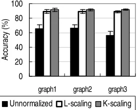
Figure 1: Generation of graph 1–5. (c,e) in the table indicates that for each node, we randomly chose c nodes of the same class and connect it to them, and we randomly chose e nodes of other classes (introducing errors) and connect it to them. Edge weights are fixed to 1.

0 20 40 60 80 100

graph1 graph2 graph3

Ac

cu

ra

cy

(%

)

Unnormalized L-scaling K-scaling

Figure 2: Classification accuracy (%) on the graphs where degrees are nearly constant within the class.

n=40,m=2000. With dimension reduction (dim_≤20; chosen by cross validation). Average over 10 random splits with one standard deviation.

first few eigenvectors of the kernel. Therefore, under certain conditions, dimension reduction can reduce noise (corresponding to a small cut), which essentially makes normalization more effective as shown in Section 3.4.

We show our formal analysis of the combination of dimension reduction (as in (6) above) and normalization of Laplacian, for completeness, in Appendix C and empirical results in the next sec-tion.

4. Experiments

We experiment with the Laplacian regularization with the normalization methods discussed above, on synthesized data sets generated by controlling graph properties as well as three real-world data sets.

4.1 Experimental Framework

The Laplacian matrix

L

is generated from a graph G so that

L

j,j0 =−w_j_,_j0 for j6= j0 and

L

_j_,_j= deg_j(G). Using

L

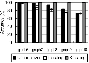
, we define matrix K as follows:

(15)

0 20 40 60 80 100

graph6 graph7 graph8 graph9 graph10

Ac

cu

ra

cy

(%

)

Figure 3: Classification accuracy on the core-satellite graphs. n=40,m=2000. With dimension reduc-tion (dim_≤20; chosen by cross validation). Average over 10 random splits with one standard deviation.

• K-scaling: K= (S−1/2(αI+

L

)S−1/2)−1_{where S}₌_diag

j(K¯−j,1j)with ¯K= (αI+

L

)−1. The

diagonal entries of K are all ones.

• L-scaling: K= (αI+S−1/2

L

S−1/2)−1_{where S}₌_diag

j(degj(G)). The diagonal entries of K−1are constant(α+1). This is the standard degree-based scaling.

Using these three types of matrix K, we test the following two types of regularization. One regu-larizes by fT_·_,_kK−1f_·,k using K without dimension reduction, as in Section 3. The other reduces the

dimension of K−1 to r by leaving out all but several eigenvectors corresponding to the smallest r eigenvalues to obtain the eigenspace projector Pr_S(G)and regularizes by:

(

fT_·_,_kK−1f_·,k if Pr_S(G)f_·,k=f_·,k

+∞ otherwise

as in Section 3.5. We use the one-versus-all strategy and use least squares as our loss function: φk(a,b) = (a−δk,b)2.

From m data points, n training labeled examples are randomly chosen while ensuring that at least one training example is chosen from each class. The remaining m₋n data points serve as test data.

The regularization parameterλis chosen by cross validation on the n training labeled examples. We will show performance when the rest of the parameters (α and dimensionality r) are also chosen by cross validation on the training labeled examples and when they are set to the optimum. The dimensionality r is chosen from K,K+5,K+10,_···,100 where K is the number of classes unless otherwise specified. Our focus is on small n close to the number of classes. Throughout this section, we conduct 10 runs with random training/test splits and report the average accuracy.

4.2 Controlled Data Experiments

The purpose of the controlled data experiments is to observe the correlation of the effectiveness of the normalization methods with graph properties. The graphs we generate contain 2000 nodes, each of which is assigned one of 10 classes.

(16)

(of either correct edges or erroneous edges) are close to constant within each class but vary across classes. Details of their generation are described in Figure 1. We observe that on these graphs, both K-scaling and L-scaling significantly improve classification accuracy over the unnormalized baseline. There is no prominent difference between K-scaling’s and L-scaling’s performance.

Observe that K-scaling and L-scaling perform differently on the graphs used in Figure 3. These graphs have the following properties. Each class consists of core nodes and satellite nodes. Core nodes of the same class are tightly connected with each other and do not have any erroneous edges. Satellite nodes are relatively weakly connected to core nodes of the same class. The satellite nodes are also connected to some other classes’ satellite nodes (i.e., introducing errors). This core-satellite model is intended to simulate real-world data in which some data points are close to the class boundaries (satellite nodes). More precisely, graphs 6–10 were generated as follows. Each graph consists of 2000 nodes (m=2000) uniformly distributed over 10 classes (K=10). 10% of the nodes are the core nodes. For every core node, we randomly choose 10 other core nodes of the same class and connect it to them with edge weight 1 (that is, each core node is connected to at least 10 core nodes of the same class). For every satellite node, we randomly choose one core node of the same class and connect them with edge weight 0.01. Also, for each satellite node, we randomly choose one satellite node of some other class (i.e., introducing error) and connect them with edge weight we. We set the error edge weight we=0.002,0.004,···,0.01 for graphs

6,7,_···,10, respectively. Note that although classes are uniformly distributed, pure components that optimize the generalization bound may be non-uniform in size. For graphs generated in this manner, degrees vary within the same class since the satellite nodes have smaller degrees than the core nodes. Our analysis suggests that L-scaling will do poorly. Figure 3 shows that on the five core-satellite graphs, K-scaling indeed produces higher performance than L-scaling. In particular,

K-scaling does well even when L-scaling rather underperforms the unnormalized baseline.

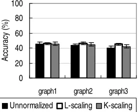
Our analysis suggests that K-scaling should work well when the graph has relatively small error. This trend is more clearly observed on these core-satellite graphs without dimension reduction. As shown in Figure 4, the advantage of K-scaling over L-scaling is more prominent on the graphs with smaller error edge weights. On the other hand, the theory suggests that when the graph has large error (large cut), the benefit of normalization is less clear (since the derivation of K-scaling assumes near-zero cut). This is especially so when dimension reduction is not applied because as pointed out in Section 3.5, dimension reduction reduces error. This trend can be observed in Figure 5, which shows that on graphs 1–3 (having larger errors than the core-satellite graphs), neither L-scaling nor K-L-scaling prominently improves performance over the unnormalized Laplacian without dimension reduction though L-scaling seems to perform slightly better. Note that the performance without dimension reduction (Figure 5) is significantly worse than the performance with dimension reduction (Figure 2). This means that dimension reduction, which reduces error, is important when we try to apply graph based methods.

(17)

80 85 90 95 100

0 0.005 0.01

Error edge weight

Ac

cu

ra

cy

(%

)

Figure 4: Classification accuracy on the core-satellite graphs. x-axis: error edge weight we. n=40,m= 2000. Without dimension reduction. Average over 10 random splits.

0 20 40 60 80 100

graph1 graph2 graph3

Ac

cu

ra

cy

(%

)

Figure 5: Classification accuracy (%) on the graphs where degrees are nearly constant within the class. Average over 10 random splits. n=40,m=2000. Without dimension reduction.

4.3 Real-world Data Experiments

Our real-world data experiments use two image data sets (MNIST and UMIST) and one text data set (RCV1).

4.3.1 DATA ANDBASELINE

The MNIST data set, downloadable from http://yann.lecun.com/exdb/mnist/, consists of hand-written digit image data (representing 10 classes, from digit “0” to “9”). For our experiments, we randomly

choose 2000 images (i.e., m = 2000). The UMIST data set, downloadable from

(18)

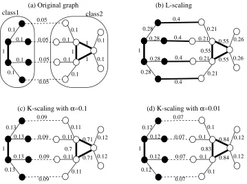
(a) Original graph (b) L-scaling

class1 _class2

(c) K-scaling with α=0.1 (d) K-scaling with α=0.01 1

0.1 0.1

0.1

0.1 0.1

1

0.05 0.1

0.1

0.1 0.05

0.05

0.05 0.1

0.1

1 1

1

0.28 0.28

0.28

0.21 0.28

0.55

0.4

0.21

0.21 0.4

0.4

0.4 0.26

0.26

0.55 0.55

1

0.13 0.13

0.13

0.11 0.13

0.7

0.09

0.11

0.11 0.09

0.09

0.09 0.12

0.12

0.71 0.71

1

0.12 0.12

0.12

0.1 0.12

0.83

0.07 0.1

0.1

0.1 0.07

0.07

0.07 0.12

0.12

0.84 0.84

Figure 6: Illustrative toy examples of scaled adjacency matrices S−1/2WS−1/2where S is derived from L-scaling or K-L-scaling. For the two-class core-satellite graph in (a), L-L-scaling makes the weights of error edges larger than the edge weights between the core nodes and satellite nodes of the same class as in (b). K-scaling does not suffer from this problem ((c),(d)). (For an easy comparison, in (b)–(d), edge weights are multiplied with constants so that the largest weight becomes one.)

To generate graphs from the image data, as is commonly done, we first generate the vectors of the gray-scale values of the pixels, and produce the edge weight between the i-th and the j-th data points Xi and Xj by wi,j =exp(−||Xi−Xj||2/t)where t>0 is a parameter (radial basis function

(RBF) kernels). To generate graphs from the text data, we first create the bag-of-word vectors using content words only2 and then set wi,j based on RBF as above or set wi,j to the inner product of Xi and Xj (linear kernels). Optionally, we zero out all wi,j but k nearest neighbors (i.e., i is j’s k

nearest neighbors or j is i’s k nearest neighbors) to reduce error in graphs and refer to it as the RBF (or linear) kernel with kNN.

As our baseline, we also test the supervised configuration by letting W+βI (where W is a

weight matrix whose(i,j)-entry is wi,j) be the kernel matrix and using the same least squares loss

function. We setβto the optimum, which was 0.001 for the RBF kernel for RCV1 and 1 for the other graphs.

(19)

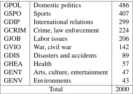
GPOL Domestic politics 486

GSPO Sports 407

GDIP International relations 299

GCRIM Crime, law enforcement 224

GJOB Labor issues 206

GVIO War, civil war 142

GDIS Disasters and accidents 89

GHEA Health 57

GENT Arts, culture, entertainment 47

GENV Environments 43

Total 2000

Figure 7: 10 RCV1 categories and their populations used in our experiments.

45 50 55 60 65 70 75 80 85

10 30 50

# of labeled examples

a

c

u

ra

c

y

(

%

)

45 50 55 60 65 70 75 80 85

10 30 50

a

c

u

ra

c

y

(

%

)

K-scaling (w/ dim reduction)

L-scaling (w/ dim reduction)

Unnormalized (w/ dim redu.)

K-scaling

L-scaling

Unnormalized

Supervised baseline (a) MNIST, dim and alpha

determined by cross validation

(b) MNIST, w/ optimum dim and optimum alpha

Figure 8: Classification accuracy (%) in relation to the number of labeled examples (n) on MNIST. m=

2000. (a) Dimensionality andαwere determined by cross validation. (b) Dimensionality andα were set to the optimum. Average over 10 random splits.

4.3.2 RESULTS

(20)

30 35 40 45 50 55 60 65 70

10 30 50 70 90 110

a c c u ra c y ( % ) 35 40 45 50 55 60 65 70 75

10 30 50 70 90 110 # of labeled examples

a c c u ra c y ( % )

K-scaling (w/ dim reduction) L-scaling (w/ dim reduction) Unnormalized (w/ dim redu.) K-scaling

L-scaling Unnormalized Supervised baseline

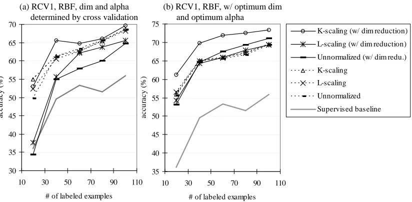
(a) RCV1, RBF, dim and alpha determined by cross validation

(b) RCV1, RBF, w/ optimum dim and optimum alpha

Figure 9: Classification accuracy (%) in relation to the number of labeled examples (n) on RCV1. RBF kernel (with t=0.25). m=2000. (a) Dimensionality andαwere determined by cross validation. (b) Dimensionality andαwere set to the optimum. Performance differences of the best performing method ‘K-scaling (w/ dim reduction)’ from ‘L-scaling (w/ dim reduction)’ and ‘Unnormalized (w/ dim redu.)’ are statistically significant (p_≤0.01) in both the settings (a) and (b).

45 50 55 60 65 70 75 80

10 30 50 70 90 110

a c c u ra c y ( % ) 45 50 55 60 65 70 75 80 85

10 30 50 70 90 110

a c c u ra c y ( % )

(a) RCV1, linear, dim and alpha determined by cross validation

(b) RCV1, linear, w/ optimum dim and optimum alpha

(21)

45 50 55 60 65 70 75 80 85 90 95

20 40 60 80

a

c

u

ra

c

y

(

%

)

45 50 55 60 65 70 75 80 85 90 95

20 40 60 80

a

c

u

ra

c

y

(

%

)

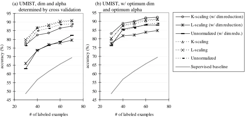
(a) UMIST, dim and alpha determined by cross validation

(b) UMIST, w/ optimum dim and optimum alpha

Figure 11: Classification accuracy (%) in relation to the number of labeled examples (n) on UMIST. m=

575. (a) Dimensionality andαwere determined by cross validation. (b) Dimensionality and

α were set to the optimum. In (b), performance differences of the best performing method ‘K-scaling (w/ dim reduction)’ from the second and third best ‘K-scaling’ and ‘L-scaling’ are statistically significant (p_≤0.01).

and K-scaling still improve performance over the unnormalized Laplacian, the best performance is always obtained by K-scaling with dimension reduction (the bold line with circles).

In Figure 8 (a), the unnormalized Laplacian with dimension reduction underperforms the un-normalized Laplacian without dimension reduction, indicating that dimension reduction rather de-grades performance in this case. By comparing Figure 8 (a) and (b), we observe that this seemingly counter-intuitive performance trend is caused by the difficulty in choosing the right dimensionality by cross validation. Figure 8 (b) shows the performance at the optimum dimensionality and the optimum α. As observed, if the optimum dimensionality is known (as in (b)), dimension reduc-tion improves performance either with or without normalizareduc-tion by K-scaling and L-scaling, and that all the transductive configurations outperform the supervised baseline. We also note that the comparison of Figure 8 (a) and (b) shows that choosing good dimensionality by cross validation is much harder than choosingαby cross validation especially when the number of labeled examples is small. This trend was observed also on the other data sets on which we experimented.

On the RCV1 data set, the performance trend is essentially similar to that of MNIST. Figure 9 shows the performance on RCV1 using the RBF kernel (t=0.25, 100NN). In the setting of Figure 9 (a) where the dimensionality andαwere determined by cross validation, K-scaling with dimension reduction generally performs the best. By setting the dimensionality and α to the optimum, the benefit of K-scaling with dimension reduction is even clearer (Figure 9 (b)).

(22)

and ‘Unnormalized (w/ dim redu.)’ are statistically significant (p≤0.01) in both Figure 10 (a) and (b).

In Figure 11, we observe that dimension reduction seems less useful on the UMIST data set. We conjecture that this may be because UMIST differs from our other data sets in that it is much more ‘sparse’; UMIST has a smaller number of data points (m=575 vs. m=2000) while it has more classes (K =20 vs. K=10). Nevertheless, when the dimensionality andα are set to the optimum (Figure 11 (b)), again, K-scaling with dimension reduction performs the best. Its differences from the second and the third best methods (K-scaling without dimension reduction and

L-scaling without dimension reduction) are statistically significant (p≤0.01).

Overall, on these graphs generated from image and text data sets, K-scaling with dimension reduction consistently outperformed the others. But without dimension reduction, K-scaling and

L-scaling were not always effective. Transductive learning (either with or without normalization)

generally improved performance.

4.4 Approximation of K-scaling

Although K-scaling consistently improves performance as shown above, its drawback is the rela-tively large runtime as it involves the computation of the inverse of an m-by-m matrix. We propose a less computationally-intensive approximation method using a known fact that(I₋A)−1₌_∑∞

k=0Ak

if_||A_||2<1. As in the introduction, let D=diagi(degi(G)), and let W be a weight matrix such that Wi,j=wi,jso that we can write

L

=D−W. Let ˆD=D+αI. We define ˆK(h)to be the h-th order

approximation of ¯K= (

L

+αI)−1_{as follows:}

ˆ

K(h) =_Dˆ−1/2

∑

h k=0

ˆ

D−1/2W ˆD−1/2

k !

ˆ

D−1/2.

We then set the i-th scaling factor Siso that:

Si=Kˆ(h)−_i_,_i1.

Since limh→∞Kˆ(h) =K, the scaling factors produced with a sufficiently large h closely approximate¯

K-scaling. On the other hand, since ˆK(0) =Dˆ−1= (D+αI)−1_{, the scaling factors produced by ˆ}_K₍₀₎

withα=0 are exactly the same as L-scaling (or the standard degree-scaling).

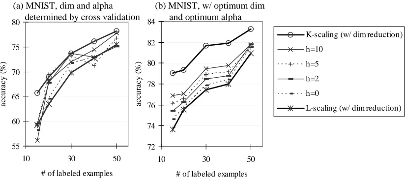
Figure 12 shows the performance of this approximation method with h=0,2,5,10 with dimen-sion reduction in comparison with corresponding K-scaling and L-scaling on MNIST. In Figure 12 (b), we observe that at the optimum dimensionality andα, the performance of the approximation method lies exactly between that of L-scaling and K-scaling, and it approaches to K-scaling as the order h increases. Intuitively, with a larger h, this approximation method takes more and more global connections into account and improves performance.

5. Conclusion

(23)

(a) MNIST, dim and alpha determined by cross validation

(b) MNIST, w/ optimum dim and optimum alpha

55 60 65 70 75 80

10 30 50

a

c

u

ra

c

y

(

%

)

72 74 76 78 80 82 84

10 30 50

a

c

u

ra

c

y

(

%

)

K-scaling (w/ dim reduction)

h=10

h=5

h=2

h=0

L-scaling (w/ dim reduction)

Figure 12: Classification accuracy (%) of the approximation method using ˆK(h). MNIST. (a) Dimension-ality and α were determined by cross validation. (b) Dimensionality and α were set to the optimum.

can vary significantly within a pure component. An alternate normalization method, which we call

K-scaling, is proposed to remedy the problem. Experiments confirm the superiority of K-scaling

combined with dimension reduction. Finally, there are possible extensions of this work that require further investigation, for example, how to use the K-scaling for other types of graphs such as direct graphs, and how to apply this idea to spectral clustering.

Appendix A. Proof of Theorem 1

The proof employs the stability analysis of Zhang (2003), and is similar to the proof of a related bound for binary-classification in Zhang and Ando (2006). We shall introduce the following nota-tion. let in+16=i1, . . . ,in be an integer randomly drawn from ¯Zn, and let Zn+1=Zn∪ {in+1}. Let

ˆf(Zn+1)be the semi-supervised learning method (1) using training data in Zn+1:

ˆf(Zn+1) =arg min

f∈RmK

"

1

n _j_∈

∑

_Z

n+1

φ(fj,yj) +λfTQKf

#

.

We have the following stability lemma (a related result can be found in Zhang, 2003);

Lemma 8 The following inequality holds for each k=1, . . . ,K:

|fîn+1,k(Zn+1)−fîn+1,k(Zn)| ≤ |∇1,kφ(fîn+1(Zn+1),yin+1)|Kin+1,in+1/(2λn),

where∇1,kφ(fi,y)denotes a sub-gradient ofφ(fi,y)with respect to fi,k, where fi= [fi,1, . . . ,fi,K]. Proof From Rockafellar (1970), we know that there exist sub-gradients∇1,kφsuch that the

follow-ing first-order condition for the optimization problem (1) holds:

−2λnK−1ˆf_·,k(Zn) =

∑

j∈Zn