Large Scale Multiple Kernel Learning

Large Scale Multiple Kernel Learning

Sören Sonnenburg SOEREN.SONNENBURG@FIRST.FRAUNHOFER.DE Fraunhofer FIRST.IDA

Kekuléstrasse 7 12489 Berlin, Germany

Gunnar Rätsch GUNNAR.RAETSCH@TUEBINGEN.MPG.DE

Friedrich Miescher Laboratory of the Max Planck Society Spemannstrasse 39

Tübingen, Germany

Christin Schäfer CHRISTIN.SCHAEFER@FIRST.FRAUNHOFER.DE Fraunhofer FIRST.IDA

Kekuléstrasse 7 12489 Berlin, Germany

Bernhard Schölkopf BERNHARDSCHOELKOPF@TUEBINGEN.MPG.DE Max Planck Institute for Biological Cybernetics

Spemannstrasse 38 72076, Tübingen, Germany

Editors: Kristin P. Bennett and Emilio Parrado-Hernández

Abstract

While classical kernel-based learning algorithms are based on a single kernel, in practice it is often desirable to use multiple kernels. Lanckriet et al. (2004) considered conic combinations of kernel matrices for classification, leading to a convex quadratically constrained quadratic program. We show that it can be rewritten as a semi-infinite linear program that can be efficiently solved by recy-cling the standard SVM implementations. Moreover, we generalize the formulation and our method to a larger class of problems, including regression and one-class classification. Experimental re-sults show that the proposed algorithm works for hundred thousands of examples or hundreds of kernels to be combined, and helps for automatic model selection, improving the interpretability of the learning result. In a second part we discuss general speed up mechanism for SVMs, especially when used with sparse feature maps as appear for string kernels, allowing us to train a string kernel SVM on a 10 million real-world splice data set from computational biology. We integrated multi-ple kernel learning in our machine learning toolboxSHOGUNfor which the source code is publicly available athttp://www.fml.tuebingen.mpg.de/raetsch/projects/shogun.

Keywords: multiple kernel learning, string kernels, large scale optimization, support vector

ma-chines, support vector regression, column generation, semi-infinite linear programming

1. Introduction

Kernel based methods such as support vector machines (SVMs) have proven to be powerful for a

wide range of different data analysis problems. They employ a so-called kernel function k(xi,xj)

learning is anα-weighted linear combination of kernels with a bias b

f(x) =sign N

∑

αiyik(xi,x) +b !

, (1)

where the xi, i=1, . . . ,N are labeled training examples (yi∈ {±1}).

Recent developments in the literature on SVMs and other kernel methods have shown the need to consider multiple kernels. This provides flexibility and reflects the fact that typical learning problems often involve multiple, heterogeneous data sources. Furthermore, as we shall see below, it leads to an elegant method to interpret the results, which can lead to a deeper understanding of the application.

While this so-called “multiple kernel learning” (MKL) problem can in principle be solved via cross-validation, several recent papers have focused on more efficient methods for multiple kernel learning (Chapelle et al., 2002; Bennett et al., 2002; Grandvalet and Canu, 2003; Ong et al., 2003; Bach et al., 2004; Lanckriet et al., 2004; Bi et al., 2004).

One of the problems with kernel methods compared to other techniques is that the resulting decision function (1) is hard to interpret and, hence, is difficult to use in order to extract relevant knowledge about the problem at hand. One can approach this problem by considering convex combinations of K kernels, i.e.

k(xi,xj) = K

∑

βkkk(xi,xj) (2)

with βk ≥0 and∑Kk=1βk =1, where each kernel kk uses only a distinct set of features. For

ap-propriately designed sub-kernels kk, the optimized combination coefficients can then be used to understand which features of the examples are of importance for discrimination: if one is able to

obtain an accurate classification by a sparse weightingβk, then one can quite easily interpret the

re-sulting decision function. This is an important property missing in current kernel based algorithms. Note that this is in contrast to the kernel mixture framework of Bennett et al. (2002) and Bi et al. (2004) where each kernel and each example are assigned an independent weight and therefore do not offer an easy way to interpret the decision function. We will illustrate that the considered MKL formulation provides useful insights and at the same time is very efficient.

We consider the framework proposed by Lanckriet et al. (2004), which results in a convex op-timization problem - a quadratically-constrained quadratic program (QCQP). This problem is more challenging than the standard SVM QP, but it can in principle be solved by general-purpose opti-mization toolboxes. Since the use of such algorithms will only be feasible for small problems with few data points and kernels, Bach et al. (2004) suggested an algorithm based on sequential mini-mization optimini-mization (SMO Platt, 1999). While the kernel learning problem is convex, it is also non-smooth, making the direct application of simple local descent algorithms such as SMO infeasi-ble. Bach et al. (2004) therefore considered a smoothed version of the problem to which SMO can be applied.

In the first part of the paper we follow a different direction: We reformulate the binary clas-sification MKL problem (Lanckriet et al., 2004) as a semi-infinite linear program, which can be efficiently solved using an off-the-shelf LP solver and a standard SVM implementation (cf. Sec-tion 2.1 for details). In a second step, we show how easily the MKL formulaSec-tion and the algorithm is generalized to a much larger class of convex loss functions (cf. Section 2.2). Our proposed

algorithm for a new loss function, it now suffices to have an LP solver and the corresponding single kernel algorithm (which is assumed to be efficient). Using this general algorithm we were able to

solve MKL problems with up to 30,000 examples and 20 kernels within reasonable time.1

We also consider a chunking algorithm that can be considerably more efficient, since it optimizes

the SVM α multipliers and the kernel coefficients βat the same time. However, for large scale

problems it needs to compute and cache the K kernels separately, instead of only one kernel as in the single kernel algorithm. This becomes particularly important when the sample size N is large. If, on the other hand, the number of kernels K is large, then the amount of memory available for caching is drastically reduced and, hence, kernel caching is not effective anymore. (The same statements also apply to the SMO-like MKL algorithm proposed in Bach et al. (2004).)

Since kernel caching cannot help to solve large scale MKL problems, we sought for ways to avoid kernel caching. This is of course not always possible, but it certainly is for the class of

kernels where the feature map Φ(x)can be explicitly computed and computations with Φ(x)can

be implemented efficiently. In Section 3.1.1 we describe several string kernels that are frequently used in biological sequence analysis and exhibit this property. Here, the feature space can be very

high dimensional, butΦ(x)is typically very sparse. In Section 3.1.2 we discuss several methods for

efficiently dealing with high dimensional sparse vectors, which not only is of interest for MKL but also for speeding up ordinary SVM classifiers. Finally, we suggest a modification of the previously proposed chunking algorithm that exploits these properties (Section 3.1.3). In the experimental part we show that the resulting algorithm is more than 70 times faster than the plain chunking algorithm (for 50,000 examples), even though large kernel caches were used. Also, we were able to solve MKL problems with up to one million examples and 20 kernels and a 10 million real-world splice site classification problem from computational biology. We conclude the paper by illustrating the usefulness of our algorithms in several examples relating to the interpretation of results and to automatic model selection. Moreover, we provide an extensive benchmark study comparing the effect of different improvements on the running time of the algorithms.

We have implemented all algorithms discussed in this work in C++ with interfaces to Matlab,

Octave, R and Python. The source code is freely available at

http://www.fml.tuebingen.mpg.de/raetsch/projects/shogun.

The examples used to generate the figures are implemented in Matlab using the Matlab

inter-face of theSHOGUN toolbox. They can be found together with the data sets used in this paper at

http://www.fml.tuebingen.mpg.de/raetsch/projects/lsmkl.

2. A General and Efficient Multiple Kernel Learning Algorithm

In this section we first derive our MKL formulation for the binary classification case and then show how it can be extended to general cost functions. In the last subsection we will propose algorithms for solving the resulting semi-infinite linear programs (SILPs).

2.1 Multiple Kernel Learning for Classification Using SILP

In the multiple kernel learning problem for binary classification one is given N data points(xi,yi) (yi∈ {±1}), where xiis translated via K mappingsΦk(x)7→RDk_{,k=1, . . . ,K, from the input into K}

feature spaces(Φ1(xi), . . . ,ΦK(xi))where Dk denotes the dimensionality of the k-th feature space. Then one solves the following optimization problem (Bach et al., 2004), which is equivalent to the

linear SVM for K=1:2

MKL Primal for Classification

min 1

2 K

∑

kwkk2 !2

+C

N

∑

ξi (3)

w.r.t. wk∈RDk,ξ∈RN,b∈R,

s.t. ξi≥0 and yi

K

∑

hwk,Φk(xi)i+b !

≥1−ξi, ∀i=1, . . . ,N

Note that the problem’s solution can be written as wk =βkw′k with βk ≥0, ∀k=1, . . . ,K and

∑K

k=1βk=1 (Bach et al., 2004). Note that therefore theℓ1-norm ofβis constrained to one, while

one is penalizing theℓ2-norm of wkin each block k separately. The idea is thatℓ1-norm constrained

or penalized variables tend to have sparse optimal solutions, whileℓ2-norm penalized variables do

not (e.g. Rätsch, 2001, Chapter 5.2). Thus the above optimization problem offers the possibility to find sparse solutions on the block level with non-sparse solutions within the blocks.

Bach et al. (2004) derived the dual for problem (3). Taking their problem (DK), squaring the

constraints on gamma, multiplying the constraints by 1₂ and finally substituting1₂γ27→γleads to the to the following equivalent multiple kernel learning dual:

MKL Dual for Classification

min γ−

N

∑

αi

w.r.t. γ∈R,α∈RN

s.t. 0≤α≤1C,

N

∑

αiyi=0

1 2

N

∑

αiαjyiyjkk(xi,xj)≤γ, ∀k=1, . . . ,K

where kk(xi,xj) =hΦk(xi),Φk(xj)i. Note that we have one quadratic constraint per kernel (Sk(α)≤

γ). In the case of K=1, the above problem reduces to the original SVM dual. We will now move

the term−∑N

i=1αi,into the constraints onγ.This can be equivalently done by adding−∑Ni=1αito both sides of the constraints and substitutingγ−∑N_i=1αi7→γ:

MKL Dual∗for Classification

min γ (4)

w.r.t. γ∈_R,α∈_RN

s.t. 0≤α≤1C,

N

∑

αiyi=0

1 2

N

∑

αiαjyiyjkk(xi,xj)− N

∑

αi

| {z }

=:Sk(α)

≤γ, ∀k=1, . . . ,K

In order to solve (4), one may solve the following saddle point problem: minimize

L

∑

βk(Sk(α)−γ) (5)

w.r.t.α∈RN,γ∈R(with 0≤α≤C1 and∑iαiyi=0), and maximize it w.r.t.β∈RK,where 0≤β. Setting the derivative w.r.t. to γto zero, one obtains the constraint∑K_k=1βk =1 and (5) simplifies to:

L

k=1βkSk(α). While one minimizes the objective w.r.t.α, at the same time one

maximizes w.r.t. the kernel weightingβ. This leads to a

Min-Max Problem

max β minα

K

∑

βkSk(α) (6)

w.r.t. α∈RN,β∈RK

s.t. 0≤α≤C , 0≤β, N

∑

αiyi=0 and K

∑

βk=1.

This problem is very similar to Equation (9) in Bi et al. (2004) when “composite kernels,“ i.e. linear

combinations of kernels are considered. There the first term of Sk(α) has been moved into the

constraint, stillβincluding the∑K_k=1βk=1 is missing.3

Assumeα∗were the optimal solution, thenθ∗:=S(α∗,β)would be minimal and, hence, S(α,β)≥

θ∗_{for allα(subject to the above constraints). Hence, finding a saddle-point of (5) is equivalent to}

solving the following semi-infinite linear program:

Semi-Infinite Linear Program (SILP)

max θ (7)

w.r.t. θ∈R,β∈RK

s.t. 0≤β,

∑

k

βk=1 and

K

∑

βkSk(α)≥θ (8)

for allα∈RN with 0≤α≤C1 and

∑

i

yiαi=0

Note that this is a linear program, as θ and β are only linearly constrained. However there are

infinitely many constraints: one for each α∈RN satisfying 0≤α≤C and∑N_i=1αiyi =0. Both

problems (6) and (7) have the same solution. To illustrate that, considerβis fixed and we minimize

αin (6). Letα∗ be the solution that minimizes (6). Then we can increase the value ofθin (7) as

long as none of the infinitely manyα-constraints (8) is violated, i.e. up toθ=∑K_k=1βkSk(α∗).On the

other hand as we increaseθfor a fixedαthe maximizingβis found. We will discuss in Section 2.3

how to solve such semi-infinite linear programs.

2.2 Multiple Kernel Learning with General Cost Functions

In this section we consider a more general class of MKL problems, where one is given an arbitrary strictly convex and differentiable loss function, for which we derive its MKL SILP formulation. We will then investigate in this general MKL SILP using different loss functions, in particular the soft-margin loss, theε-insensitive loss and the quadratic loss.

We define the MKL primal formulation for a strictly convex and differentiable loss function

L(f(x),y)as:

MKL Primal for Generic Loss Functions

min 1

2 K

∑

kwkk !2

+ N

∑

L(f(xi),yi) (9)

w.r.t. w= (w1, . . . ,wK)∈RD1× · · · ×RDK

s.t. f(xi) =

K

∑

hΦk(xi),wki+b, ∀i=1, . . . ,N

In analogy to Bach et al. (2004) we treat problem (9) as a second order cone program (SOCP) leading to the following dual (see Appendix A for the derivation):

MKL Dual∗for Generic Loss Functions

min γ (10)

w.r.t. γ∈R,α∈RN

s.t. N

∑

αi=0 and

1 2

N

∑

i=1

αiΦk(xi)

2 2

−

N

∑

i=1

L(L′−1(αi,yi),yi) + N

∑

i=1

αiL′−1(αi,yi)≤γ,∀k=1, . . . ,K

SILP for Generic Loss Functions

max θ (11)

w.r.t. θ∈R,β∈RK

s.t. 0≤β,

K

∑

βk=1 and K

∑

βkSk(α)≥θ,∀α∈RN, N

∑

αi=0,

where

Sk(α) =− N

∑

L(L′−1(αi,yi),yi) + N

∑

αiL′−1(αi,yi) + 1 2 N

∑

αiΦk(xi) 2 2 .

We assumed that L(x,y)is strictly convex and differentiable in x. Unfortunately, the soft margin and

ε-insensitive loss do not have these properties. We therefore consider them separately in the sequel.

Soft Margin Loss We use the following loss in order to approximate the soft margin loss:

Lσ(x,y) =C

σlog(1+exp(σ(1−xy))).

It is easy to verify that

lim

σ→∞Lσ(x,y) =C(1−xy)+.

Moreover, L_σ is strictly convex and differentiable for σ<∞. Using this loss and assuming yi∈

{±1}, we obtain (cf. Appendix B.3):

Sk(α) =− N

∑

i=1 C σ log Cyi

αi+Cyi

+log

−_α αi

i+Cyi

+

N

∑

i=1

αiyi+

1 2 N

∑

i=1

αiΦk(xi)

2 2 .

Ifσ→∞, then the first two terms vanish provided that−C≤αi ≤0 if yi=1 and 0≤αi ≤C if

yi=−1. Substitutingαi=−α˜iyi, we obtain

Sk(α˜) =−

N

∑

1 2 N

∑

αiyiΦk(xi) 2 2 and N

∑

αiyi=0,

with 0≤α˜i≤C (i=1, . . . ,N) which is the same as (7).

One-Class Soft Margin Loss The one-class SVM soft margin (e.g. Schölkopf and Smola, 2002) is very similar to the two-class case and leads to

Sk(α) = 1 2 N

∑

αiΦk(xi) 2 2

subject to 0≤α≤ 1

νN1 and∑ N

ε-insensitive Loss Using the same technique for the epsilon insensitive loss L(x,y) =C(1− |x− y|)+, we obtain

Sk(α,α∗) = 1 2

N

∑

(αi−α∗i)Φk(xi) 2 2

−

N

∑

(αi+α∗i)ε− N

∑

(αi−α∗i)yi

and N

∑

(αi−α∗i)yi=0, with 0≤α,α∗≤C1.

It is easy to derive the dual problem for other loss functions such as the quadratic loss or logistic loss (see Appendix B.1 & B.2). Note that the dual SILP’s only differ in the definition of Skand the

domains of theα’s.

2.3 Algorithms to Solve SILPs

All semi-infinite linear programs considered in this work have the following structure:

max θ (12)

w.r.t. θ∈R,β∈RK

s.t. 0≤β,

K

∑

βk=1 and K

∑

βkSk(α)≥θfor allα∈

C

They have to be optimized with respect to β and θ. The constraints depend on definition of Sk

and therefore on the choice of the cost function. Using Theorem 5 in Rätsch et al. (2002) one can show that the above SILP has a solution if the corresponding primal is feasible and bounded (see also Hettich and Kortanek, 1993). Moreover, there is no duality gap, if

M

C

We propose to use a technique called Column Generation to solve (12). The basic idea is to compute the optimal(β,θ) in (12) for a restricted subset of constraints. It is called the restricted

master problem. Then a second algorithm generates a new, yet unsatisfied constraint determined by

α. In the best case the other algorithm finds the constraint that maximizes the constraint violation

for the given intermediate solution(β,θ), i.e.

αβ:=argmin

α∈C

∑

βkSk(α). (13)

Ifα_βsatisfies the constraint∑K_k=1βkSk(αβ)≥θ, then the solution(θ,β)is optimal. Otherwise, the constraint is added to the set of constraints and the iterations continue.

Algorithm 1 is a special case of a set of SILP algorithms known as exchange methods. These methods are known to converge (cf. Theorem 7.2 in Hettich and Kortanek, 1993). However, no

convergence rates for such algorithm are known.4

Since it is often sufficient to obtain an approximate solution, we have to define a suitable con-vergence criterion. Note that the problem is solved when all constraints are satisfied. Hence, it is a

4. It has been shown that solving semi-infinite problems like (7), using a method related to boosting (e.g. Meir and Rätsch, 2003) one requires at most T=O(log(M)/ˆε2_{)iterations, where ˆεis the remaining constraint}

natural choice to use the normalized maximal constraint violation as a convergence criterion, i.e. the

algorithm stops ifεMKL≥εtMKL:=

1−∑

K

k=1βtkSk(αt)

θt

, whereεMKLis an accuracy parameter,(βt,θt)

is the optimal solution at iteration t−1 andαt corresponds to the newly found maximally violating

constraint of the next iteration.

In the following we will formulate algorithms that alternately optimize the parametersαandβ.

2.3.1 A WRAPPERALGORITHM

The wrapper algorithm (see Algorithm 1) divides the problem into an inner and an outer subproblem. The solution is obtained by alternatively solving the outer problem using the results of the inner problem as input and vice versa until convergence. The outer loop constitutes the restricted master

problem which determines the optimalβfor a fixedαusing an of-the-shelf linear optimizer. In the inner loop one has to identify unsatisfied constraints, which, fortunately, turns out to be particularly simple. Note that (13) is for all considered cases exactly the dual optimization problem of the single

kernel case for fixedβ. For instance for binary classification with soft-margin loss, (13) reduces to

the standard SVM dual using the kernel k(xi,xj) =∑kβkkk(xi,xj):

v= min

α∈RN

N

∑

αiαjyiyjk(xi,xj)− N

∑

αi

s.t. 0≤α≤C1 and

N

∑

αiyi=0.

Hence, we can use a standard SVM implementation with a single kernel in order to identify the most violated constraint v≤θ. Since there exists a large number of efficient algorithms to solve the single kernel problems for all sorts of cost functions, we have therefore found an easy way to extend their applicability to the problem of Multiple Kernel Learning. Also, if the kernels are computed on-the-fly within the SVM still only a single kernel cache is required. The wrapper algorithm is very easy to implement, very generic and already reasonably fast for small to medium size problems. However,

determiningαup to a fixed high precision even for intermediate solutions, whileβis still far away

from the global optimal is unnecessarily costly. Thus there is room for improvement motivating the next section.

2.3.2 A CHUNKINGALGORITHM FORSIMULTANEOUSOPTIMIZATION OFαANDβ

The goal is to simultaneously optimizeαandβin SVM training. Usually it is infeasible to use

stan-dard optimization tools (e.g. MINOS, CPLEX, LOQO) for solving even the SVM training problems on data sets containing more than a few thousand examples. So-called decomposition techniques as chunking (e.g. used in Joachims, 1998) overcome this limitation by exploiting the special structure of the SVM problem. The key idea of decomposition is to freeze all but a small number of opti-mization variables (working set) and to solve a sequence of constant-size problems (subproblems of the SVM dual).

Here we would like to propose an extension of the chunking algorithm to optimize the kernel

weightsβand the example weightsαat the same time. The algorithm is motivated from an

insuf-ficiency of the wrapper algorithm described in the previous section: If theβ’s are not optimal yet,

Algorithm 1 The MKL-wrapper algorithm optimizes a convex combination of K kernels and em-ploys a linear programming solver to iteratively solve the semi-infinite linear optimization problem

(12). The accuracy parameterεMKLis a parameter of the algorithm. Sk(α)and

C

the cost function.

S0=1,θ1=−∞,β1_k=_K1 for k=1, . . . ,K

for t=1,2, . . .do

Computeαt=argmin α∈C

K

∑

k=1

βt

kSk(α)by single kernel algorithm with k= K

∑

k=1

βt

kkk

St=

K

∑

k=1

βt

kStk, where Stk=Sk(αt)

if

1−

St

θt

≤εMKLthen break

(βt+1,θt+1_{) =argmaxθ} w.r.t. β∈RK,θ∈R

s.t. 0≤β,

K

∑

k=1

βk=1 and K

∑

k=1

βkSrk≥θfor r=1, . . . ,t

end for

be considerably faster if for any newly obtainedαin the chunking iterations, we could efficiently

recompute the optimalβand then continue optimizing theα’s using the new kernel weighting.

Intermediate Recomputation of β Recomputing β involves solving a linear program and the

problem grows with each additional α-induced constraint. Hence, after many iterations solving

the LP may become infeasible. Fortunately, there are two facts making it still possible: (a) only a small number of the added constraints remain active and one may as well remove inactive ones — this prevents the LP from growing arbitrarily and (b) for Simplex-based LP optimizers such as

CPLEXthere exists the so-called hot-start feature which allows one to efficiently recompute the new

solution, if for instance only a few additional constraints are added.

The SVMlightoptimizer which we are going to modify, internally needs the output

ˆ

gi= N

∑

αjyjk(xi,xj)

for all training examples i=1, . . . ,N in order to select the next variables for optimization (Joachims,

1999). However, if one changes the kernel weights, then the stored ˆgi values become invalid and

need to be recomputed. In order to avoid the full recomputation one has to additionally store a K×N

matrix gk,i=∑Nj=1αjyjkk(xi,xj), i.e. the outputs for each kernel separately. If theβ’s change, then ˆgi can be quite efficiently recomputed by ˆgi=∑kβkgk,i. We implemented the final chunking algorithm for the MKL regression and classification case and display the latter in Algorithm 2.

2.3.3 DISCUSSION

The Wrapper as well as the chunking algorithm have both their merits: The Wrapper algorithm only relies on the repeated efficient computation of the single kernel solution, for which typically

large scale algorithms exist. The chunking algorithm is faster, since it exploits the intermediateα’s

Algorithm 2 Outline of the MKL-chunking algorithm for the classification case (extension to SVMlight) that optimizes α and the kernel weighting β simultaneously. The accuracy parameter

εMKLand the subproblem size Q are assumed to be given to the algorithm. For simplicity we omit

the removal of inactive constraints. Also note that from one iteration to the next the LP only differs by one additional constraint. This can usually be exploited to save computing time for solving the LP.

gk,i=0, ˆgi=0,αi=0,β1k=K1 for k=1, . . . ,K and i=1, . . . ,N

for t=1,2, . . .do

Check optimality conditions and stop if optimal

select Q suboptimal variables i1, . . . ,iQbased on ˆg andα

αold_=α

solve SVM dual with respect to the selected variables and updateα gk,i=gk,i+∑Qq=1(αiq−α

old

iq )yiqkk(xiq,xi)for all k=1, . . . ,M and i=1, . . . ,N

for k=1, . . . ,K do St

k= 1

2∑rgk,rαtryr−∑rαtr

end for

St=∑K k=1βtkS

t k

if

1−S

t

θt

≥εMKL

(βt+1,θt+1_{) =argmaxθ} w.r.t.β∈RK,θ∈R

s.t. 0≤β, ∑kβk=1 and∑Mk=1βkSkr≥θfor r=1, . . . ,t

else

θt+1_=θt

end if

ˆ

gi=∑kβkt+1gk,ifor all i=1, . . . ,N

end for

N is large). If, on the other hand, K is large, then the amount of memory available for caching

is drastically reduced and, hence, kernel caching is not effective anymore. The same statements also apply to the SMO-like MKL algorithm proposed in Bach et al. (2004). In this case one is left with the Wrapper algorithm, unless one is able to exploit properties of the particular problem or the sub-kernels (see next section).

3. Sparse Feature Maps and Parallel Computations

In this section we discuss two strategies to accelerate SVM training. First we consider the case

where the explicit mappingΦinto the kernel feature space is known as well as sparse. For this case

we show that MKL training (and also SVM training in general) can be made drastically faster, in particular, when N and K are large. In the second part we discuss a simple, yet efficient way to parallelize MKL as well as SVM training.

3.1 Explicit Computations with Sparse Feature Maps

We assume that all K sub-kernels are given as

and the mappingsΦk are given explicitly (k=1, . . . ,K). Moreover, we suppose that the mapped

examples Φk(x) are very sparse. We start by giving examples of such kernels and discuss two

kernels that are often used in biological sequence analysis (Section 3.1.1). In Section 3.1.2 we discuss several strategies for efficiently storing and computing with high dimensional sparse vectors (in particular for these two kernels). Finally in Section 3.1.3 we discuss how we can exploit these

properties to accelerate chunking algorithms, such as SVMlight, by a factor of up to Q (the chunking

subproblem size).

3.1.1 STRINGKERNELS

The Spectrum Kernel The spectrum kernel (Leslie et al., 2002) implements the n-gram or bag-of-words kernel (Joachims, 1998) as originally defined for text classification in the context of bio-logical sequence analysis. The idea is to count how often a d-mer (a contiguous string of length d)

is contained in the sequences x and x′. Summing up the product of these counts for every possible

d-mer (note that there are exponentially many) gives rise to the kernel value which formally is

de-fined as follows: LetΣbe an alphabet and u∈Σd _{a d-mer and #u(x)the number of occurrences of}

u in x. Then the spectrum kernel is defined as the inner product of k(x,x′) =hΦ(x),Φ(x′_{)i, where}

Φ(x) = (#u(x))_u∈Σd. Note that spectrum-like kernels cannot extract any positional information from

the sequence which goes beyond the d-mer length. It is well suited for describing the content of a sequence but is less suitable for instance for analyzing signals where motifs may appear in a cer-tain order or at specific positions. Also note that spectrum-like kernels are capable of dealing with sequences with varying length.

The spectrum kernel can be efficiently computed in

O

2002), where|x|denotes the length of sequence x. An easier way to compute the kernel for two

sequences x and x′ is to separately extract and sort the N d-mers in each sequence, which can be

done in a preprocessing step. Note that for instance DNA d-mers of length d≤16 can be efficiently

represented as a 32-bit integer value. Then one iterates over all d-mers of sequences x and x′

simultaneously and counts which d-mers appear in both sequences and sums up the product of their counts. The computational complexity of the kernel computation is

O

The Weighted Degree Kernel The so-called weighted degree (WD) kernel (Rätsch and Sonnenburg, 2004) efficiently computes similarities between sequences while taking positional information of k-mers into account. The main idea of the WD kernel is to count the (exact) co-occurrences of k-k-mers at corresponding positions in the two sequences to be compared. The WD kernel of order d

com-pares two sequences xiand xj of length L by summing all contributions of k-mer matches of lengths

k∈ {1, . . . ,d}, weighted by coefficientsβk:

k(xi,xj) = d

∑

βk L−k+1

∑

I(uk,l(xi) =uk,l(xj)). (14)

Here, uk,l(x)is the string of length k starting at position l of the sequence x and I(·)is the indicator function which evaluates to 1 when its argument is true and to 0 otherwise. For the weighting coefficients, Rätsch and Sonnenburg (2004) proposed to useβk=2_dd₍−_dk₊+₁1₎.Matching substrings are

thus rewarded with a score depending on the length of the substring.5

5. Note that although in our caseβk+1<βk, longer matches nevertheless contribute more strongly than shorter ones: this

Note that the WD kernel can be understood as a Spectrum kernel where the k-mers starting at

different positions are treated independently of each other.6 Moreover, it does not only consider

substrings of length exactly d, but also all shorter matches. Hence, the feature space for each position has∑d_k=1|Σ|k₌|Σ|d+1−1

|Σ|−1 −1 dimensions and is additionally duplicated L times (leading to

O

case

O

3.1.2 EFFICIENT STORAGE OFSPARSEWEIGHTS

The considered string kernels correspond to a feature space that can be huge. For instance in the

case of the WD kernel on DNA sequences of length 100 with K=20, the corresponding feature

space is 1014dimensional. However, most dimensions in the feature space are not used since only

a few of the many different k-mers actually appear in the sequences. In this section we briefly discuss three methods to efficiently deal with sparse vectors v. We assume that the elements of the

vector v are indexed by some index set

U

U

operations:clear,addandlookup. The first operation sets the vector v to zero, theaddoperation

increases the weight of a dimension for an element u∈

U

lookuprequests the value vu. The latter two operations need to be performed as quickly as possible

(whereas the performance of thelookupoperation is of higher importance).

Explicit Map If the dimensionality of the feature space is small enough, then one might consider keeping the whole vector v in memory and to perform direct operations on its elements. Then each read or write operation is

O

_O

is very fast and best suited for instance for the Spectrum kernel on DNA sequences with d≤14 and

on protein sequences with d≤6.

Sorted Arrays More memory efficient but computationally more expensive are sorted arrays of

index-value pairs(u,vu). Assuming the L indexes are given and sorted in advance, one can

effi-ciently change or look up a single vufor a corresponding u by employing a binary search procedure

(

O

si-multaneously traverse the two arrays in order to determine which elements appear in the first array (i.e.

O

O

method is well suited for cases where L and L′ are of comparable size, as for instance for

compu-tations of single Spectrum kernel elements (as proposed in Leslie et al., 2004). If, L≫L′, then the

binary search procedure should be preferred.

Tries Another way of organizing the non-zero elements are tries (Fredkin, 1960): The idea is to use a tree with at most|Σ|siblings of depth d. The leaves store a single value: the element vu, where

u∈Σd_{is a d-mer and the path to the leaf corresponds to u.}

knowledge allows for aO(L)reformulation of the kernel using “block-weights” as has been done in Sonnenburg et al. (2005b).

6. It therefore is very position dependent and does not tolerate any positional “shift”. For that reason we proposed in Rätsch et al. (2005) a WD kernel with shifts, which tolerates a small number of shifts, that lies in between the WD and the Spectrum kernel.

To addorlookup an element one only needs d operations to reach a leaf of the tree (and to

create necessary nodes on the way in an addoperation). Note that the worst-case computational

complexity of the operations is independent of the number of d-mers/elements stored in the tree.

While tries are not faster than sorted arrays inlookupand need considerably more storage (e.g.

for pointers to its parent and siblings), they are useful for the previously discussed WD kernel. Here

we not only have to lookup one substring u∈Σd_{, but also all prefixes of u. For sorted arrays this}

amounts to d separatelookupoperations, while for tries all prefixes of u are already known when

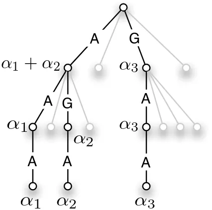
the bottom of the tree is reached. In this case the trie has to store weights also on the internal nodes. This is illustrated for the WD kernel in Figure 1.

α

₁

α

2

α

₃

α

₁

+

α

₂

α

₃

α

₃

α

1

α

2

Figure 1: Three sequences AAA, AGA, GAA with weightsα1,α2&α3are added to the trie. The

figure displays the resulting weights at the nodes.

3.1.3 SPEEDINGUPSVM TRAINING

As it is not feasible to use standard optimization toolboxes for solving large scale SVM train-ing problem, decomposition techniques are used in practice. Most chunktrain-ing algorithms work by first selecting Q variables (working set W ⊆ {1, . . . ,N}, Q :=|W|) based on the current solution and then solve the reduced problem with respect to the working set variables. These two steps are repeated until some optimality conditions are satisfied (see e.g. Joachims (1998)). For se-lecting the working set and checking the termination criteria in each iteration, the vector g with

gi=∑Nj=1αjyjk(xi,xj), i=1, . . . ,N is usually needed. Computing g from scratch in every

iter-ation which would require

O

starts with g=0 and only computes updates of g on the working set W

gi←goldi +

∑

As a result the effort decreases to

O

large scale problems8 and thus most time is spend computing kernel rows for the updates of g on

the working set W . Note however that this update as well as computing the Q kernel rows can be easily parallelized; cf. Section 4.2.1.

Exploiting k(xi,xj) =hΦ(xi),Φ(xj)iand w=∑Ni=1αiyiΦ(xi)we can rewrite the update rule as

gi←goldi +

∑

(αj−αoldj )yjhΦ(xi),Φ(xj)i=goldi +hwW,Φ(xi)i, (15)

where wW =∑_j∈W(αj−αoldj )yjΦ(xj)is the normal (update) vector on the working set.

If the kernel feature map can be computed explicitly and is sparse (as discussed before), then

computing the update in (15) can be accelerated. One only needs to compute and store wW (using

theclearand∑q∈W|{Φj(xq)=6 0}|addoperations) and performing the scalar producthwW,Φ(xi)i

(using|{Φj(xi)6=0}|lookupoperations).

Depending on the kernel, the way the sparse vectors are stored Section 3.1.2 and on the sparse-ness of the feature vectors, the speedup can be quite drastic. For instance for the WD kernel one

kernel computation requires

O

(15) N times requires O(NQLd)operations. When using tries, then one needs QL addoperations

(each

O

O

O

opera-tions are needed in total. When N is large enough it leads to a speedup by a factor of Q. Finally note

that kernel caching is no longer required and as Q is small in practice (e.g. Q=42) the resulting trie

has rather few leaves and thus only needs little storage.

The pseudo-code of ourlinaddSVM chunking algorithm is given in Algorithm 3.

Algorithm 3 Outline of the chunking algorithm that exploits the fast computations of linear combi-nations of kernels (e.g. by tries).

{INITIALIZATION}

gi=0,αi=0 for i=1, . . . ,N {LOOP UNTIL CONVERGENCE} for t=1,2, . . .do

Check optimality conditions and stop if optimal

select working set W based on g andα, storeαold=α

solve reduced problem W and updateα

clearw

w←w+ (αj−αoldj )yjΦ(xj)for all j∈W (usingadd) update gi=gi+hw,Φ(xi)ifor all i=1, . . . ,N (usinglookup) end for

MKL Case As elaborated in Section 2.3.2 and Algorithm 2, for MKL one stores K vectors gk, k=1, . . . ,K: one for each kernel in order to avoid full recomputation of ˆg if a kernel weightβk is updated. Thus to use the idea above in Algorithm 2 all one has to do is to store K normal vectors

(e.g. tries)

wW_k =

∑

(αj−αoldj )yjΦk(xj), k=1, . . . ,K

which are then used to update the K×N matrix gk,i=gold_k,i +hwW_k ,Φk(xi)i(for all k=1. . .K and

i=1. . .N) by which ˆgi=∑kβkgk,i,(for all i=1. . .N) is computed.

3.2 A Simple Parallel Chunking Algorithm

As still most time is spent in evaluating g(x)for all training examples further speedups are gained

when parallelizing the evaluation of g(x). When using thelinaddalgorithm, one first constructs

the trie (or any of the other possible more appropriate data structures) and then performs parallel

lookup operations using several CPUs (e.g. using shared memory or several copies of the data

structure on separate computing nodes). We have implemented this algorithm based on multiple

threads (using shared memory) and gain reasonable speedups (see next section).

Note that this part of the computations is almost ideal to distribute to many CPUs, as only the

updatedα(or w depending on the communication costs and size) have to be transfered before each

CPU computes a large chunk Ik⊂ {1, . . . ,N}of

h(_ik)=hw,Φ(xi)i, ∀i∈Ik, ∀k=1, . . . ,N,where(I1∪ · · · ∪In) = (1, . . . ,N)

which is transfered to a master node that finally computes g←g+h,as illustrated in Algorithm 4.

4. Results and Discussion

In the following subsections we will first apply multiple kernel learning to knowledge discovery tasks, demonstrating that it can be used for automated model selection and to interpret the learned model (Section 4.1), followed by a benchmark comparing the running times of SVMs and MKL using any of the proposed algorithmic optimizations (Section 4.2).

4.1 MKL for Knowledge Discovery

In this section we will discuss toy examples for binary classification and regression, showing that MKL can recover information about the problem at hand, followed by a brief review on problems for which MKL has been successfully used.

4.1.1 CLASSIFICATION

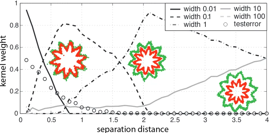
The first example we deal with is a binary classification problem. The task is to separate two concentric classes shaped like the outline of stars. By varying the distance between the boundary of the stars we can control the separability of the problem. Starting with a non-separable scenario with zero distance, the data quickly becomes separable as the distance between the stars increases, and the boundary needed for separation will gradually tend towards a circle. In Figure 2 three scatter plots of data sets with varied separation distances are displayed.

We generate several training and test sets for a wide range of distances (the radius of the inner

star is fixed at 4.0, the outer stars radius is varied from 4.1. . .9.9). Each data set contains 2,000

Algorithm 4 Outline of the parallel chunking algorithm that exploits the fast computations of linear combinations of kernels.

{ Master node } {INITIALIZATION}

gi=0,αi=0 for i=1, . . . ,N {LOOP UNTIL CONVERGENCE} for t=1,2, . . .do

Check optimality conditions and stop if optimal

select working set W based on g andα, storeαold=α

solve reduced problem W and updateα

transfer to Slave nodes:αj−αoldj for all j∈W fetch from n Slave nodes: h= (h(1)_{, . . . ,h}(n)₎

update gi=gi+hi for all i=1, . . . ,N end for

signal convergence to slave nodes

{ Slave nodes }

{LOOP UNTIL CONVERGENCE} while not converged do

fetch from Master nodeαj−αold_j for all j∈W

clearw

w←w+ (αj−αoldj )yjΦ(xj)for all j∈W (usingadd) node k computes h(_ik)=hw,Φ(xi)i

for all i= (k−1)N n, . . . ,k

N

n−1 (usinglookup)

transfer to master: h(k) end while

regularization parameter C,where we setεMKL=10−3.For every value of C we averaged the test

errors of all setups and choose the value of C that led to the smallest overall error (C=0.5).9

The choice of the kernel width of the Gaussian RBF (below, denoted by RBF) kernel used for classification is expected to depend on the separation distance of the learning problem: An increased distance between the stars will correspond to a larger optimal kernel width. This effect should be visible in the results of the MKL, where we used MKL-SVMs with five RBF kernels with

different widths (2σ2∈ {0.01,0.1,1,10,100}). In Figure 2 we show the obtained kernel weightings

for the five kernels and the test error (circled line) which quickly drops to zero as the problem becomes separable. Every column shows one MKL-SVM weighting. The courses of the kernel weightings reflect the development of the learning problem: as long as the problem is difficult the best separation can be obtained when using the kernel with smallest width. The low width kernel looses importance when the distance between the stars increases and larger kernel widths obtain a larger weight in MKL. Increasing the distance between the stars, kernels with greater widths are used. Note that the RBF kernel with largest width was not appropriate and thus never chosen. This illustrates that MKL can indeed recover information about the structure of the learning problem.

0 0.5 1 1.5 2 2.5 3 3.5 4 0

0.2 0.4 0.6 0.8 1

width 0.01 width 0.1 width 1

width 10 width 100 testerror

separation distance

ke

rnel

w

e

igh

t

Figure 2: A 2-class toy problem where the dark gray (or green) star-like shape is to be distinguished from the light gray (or red) star inside of the dark gray star. The distance between the dark star-like shape and the light star increases from the left to the right.

4.1.2 REGRESSION

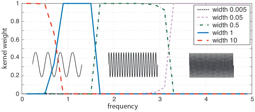
We applied the newly derived MKL support vector regression formulation to the task of learning a

sine function using three RBF-kernels with different widths (2σ2∈ {0.005,0.05,0.5,1,10}). To this

end, we generated several data sets with increasing frequency of the sine wave. The sample size was

chosen to be 1,000. Analogous to the procedure described above we choose the value of C=10,

minimizing the overall test error. In Figure 3 exemplarily three sine waves are depicted, where the frequency increases from left to right. For every frequency the computed weights for each kernel width are shown. One can see that MKL-SV regression switches to the width of the RBF-kernel fitting the regression problem best.

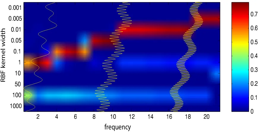
In another regression experiment, we combined a linear function with two sine waves, one

of lower frequency and one of high frequency, i.e. f(x) =sin(ax) +sin(bx) +cx.Furthermore we

increase the frequency of the higher frequency sine wave, i.e. we varied a leaving b and c unchanged. The MKL weighting should show a combination of different kernels. Using ten RBF-kernels of different width (see Figure 4) we trained a MKL-SVR and display the learned weights (a column

in the figure). Again the sample size is 1,000 and one value for C=5 is chosen via a previous

experiment (εMKL=10−5). The largest selected width (100) models the linear component (since

0 1 2 3 4 5 0

0.2 0.4 0.6 0.8 1

width 0.005 width 0.05 width 0.5 width 1 width 10

frequency

ke

rnel w

eig

h

t

Figure 3: MKL-Support Vector Regression for the task of learning a sine wave (please see text for details).

Additionally one can observe that MKL leads to sparse solutions since most of the kernel weights in Figure 4 are depicted in blue, that is they are zero.10

4.1.3 REALWORLDAPPLICATIONS INBIOINFORMATICS

MKL has been successfully used on real-world data sets in the field of computational biology (Lanckriet et al., 2004; Sonnenburg et al., 2005a). It was shown to improve classification perfor-mance on the task of ribosomal and membrane protein prediction (Lanckriet et al., 2004), where a weighting over different kernels each corresponding to a different feature set was learned. In their result, the included random channels obtained low kernel weights. However, as the data sets was

rather small (≈1,000 examples) the kernel matrices could be precomputed and simultaneously kept

in memory, which was not possible in Sonnenburg et al. (2005a), where a splice site recognition task for the worm C. elegans was considered. Here data is available in abundance (up to one million ex-amples) and larger amounts are indeed needed to obtain state of the art results (Sonnenburg et al.,

2005b).11 On that data set we were able to solve the classification MKL SILP for N=1,000,000

examples and K=20 kernels, as well as for N=10,000 examples and K=550 kernels, using the

linadd optimizations with the weighted degree kernel. As a result we a) were able to learn the

weightingβinstead of choosing a heuristic and b) were able to use MKL as a tool for interpreting

the SVM classifier as in Sonnenburg et al. (2005a); Rätsch et al. (2005).

As an example we learned the weighting of a WD kernel of degree 20, which consist of a

weighted sum of 20 sub-kernels each counting matching d-mers, for d=1, . . . ,20.The learned

10. The training time for MKL-SVR in this setup but with 10,000 examples was about 40 minutes, when kernel caches of size 100MB are used.

frequency

RBF kernel width

2 4 6 8 1 0 1 2 1 4 1 6 1 8 2 0

0 .0 0 1

0 .0 0 5

0 .0 1

0 .0 5

0 .1

1

1 0

5 0

1 0 0

1 0 0 0

0

0 .1 0 .2 0 .3 0 .4 0 .5 0 .6 0 .7

Figure 4: MKL support vector regression on a linear combination of three functions: f(x) =

sin(ax) +sin(bx) +cx. MKL recovers that the original function is a combination of

func-tions of low and high complexity. For more details see text.

0 5 10 15 20 25

0 0.05

0.1 0.15

0. 2 0.25 0. 3 0.35

kernel index d _{(length of substring)}

ke

rnel w

eig

ht

Figure 5: The learned WD kernel weighting on a million of examples.

quite different properties, i.e. the 9th and 10th kernel leads to a combined kernel matrix that is most diagonally dominant (since the sequences are only similar to themselves but not to other sequences),

which we believe is the reason for having a large weight.12

In the following example we consider one weight per position. In this case the combined ker-nels are more similar to each other and we expect more interpretable results. Figure 6 shows an

−50 −40 −30 −20 −10 Exon Start

+10 +20 +30 +40 +50 0

0.005 0.01 0.015

0.02 0.025

0.03 0.035

0.04 0.045

0.05

ke

rnel w

eig

ht

position relative to the exon start

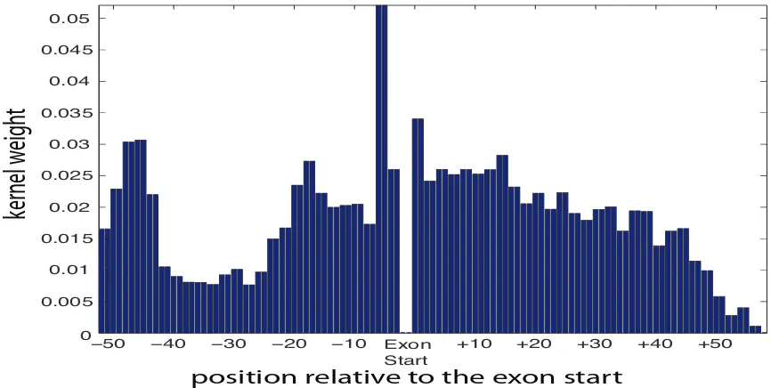
Figure 6: The figure shows an importance weighting for each position in a DNA sequence (around a so called splice site). MKL was used to determine these weights, each corresponding to a sub-kernel which uses information at that position to discriminate splice sites from non-splice sites. Different peaks correspond to different biologically known signals (see text for details). We used 65,000 examples for training with 54 sub-kernels.

importance weighting for each position in a DNA sequence (around a so called acceptor splice site, the start of an exon). We used MKL on 65,000 examples to compute these 54 weights, each cor-responding to a sub-kernel which uses information at that position to discriminate true splice sites from fake ones. We repeated that experiment on ten bootstrap runs of the data set. We can iden-tify several interesting regions that we can match to current biological knowledge about splice site

recognition: a) The region −50 nucleotides (nt) to−40nt, which corresponds to the donor splice

site of the previous exon (many introns in C. elegans are very short, often only 50nt), b) the region

−25nt to−15nt that coincides with the location of the branch point, c) the intronic region closest

to the splice site with greatest weight (−8nt to−1nt; the weights for theAGdimer are zero, since

it appears in splice sites and decoys) and d) the exonic region (0nt to+50nt). Slightly surprising

are the high weights in the exonic region, which we suspect only model triplet frequencies. The

decay of the weights seen from+15nt to+45nt might be explained by the fact that not all exons are

actually long enough. Furthermore, since the sequence ends in our case at+60nt, the decay after

+45nt is an edge effect as longer substrings cannot be matched.

4.2 Benchmarking the Algorithms

Experimental Setup To demonstrate the effect of the several proposed algorithmic

optimiza-tions, namely the linadd SVM training (Algorithm 3) and for MKL the SILP formulation with

and without thelinadd extension for single, four and eight CPUs, we applied each of the

algo-rithms to a human splice site data set,13 comparing it to the original WD formulation and the case

where the weighting coefficients were learned using multiple kernel learning. The splice data set contains 159,771 true acceptor splice site sequences and 14,868,555 decoys, leading to a total of 15,028,326 sequences each 141 base pairs in length. It was generated following a procedure similar to the one in Sonnenburg et al. (2005a) for C. elegans which however contained “only” 1,026,036 examples. Note that the data set is very unbalanced as 98.94% of the examples are negatively la-beled. We are using this data set in all benchmark experiments and trained (MKL-)SVMs using

the SHOGUN machine learning toolbox which contains a modified version of SVMlight (Joachims,

1999) on 500, 1,000, 5,000, 10,000, 30,000, 50,000, 100,000, 200,000, 500,000, 1,000,000,

2,000,000, 5,000,000 and 10,000,000 randomly sub-sampled examples and measured the time

needed in SVM training. For classification performance evaluation we always use the same

re-maining 5,028,326 examples as a test data set. We set the degree parameter to d=20 for the WD

kernel and to d =8 for the spectrum kernel fixing the SVMs regularization parameter to C=5.

Thus in the MKL case also K=20 sub-kernels were used. SVMlight’s subproblem size (parameter

qpsize), convergence criterion (parameterepsilon) and MKL convergence criterion were set to

Q=112,εSV M =10−5 and εMKL=10−5, respectively. A kernel cache of 1GB was used for all

kernels except the precomputed kernel and algorithms using thelinadd-SMO extension for which

the kernel-cache was disabled. Later on we measure whether changing the quadratic subproblem size Q influences SVM training time. Experiments were performed on a PC powered by eight 2.4GHz AMD Opteron(tm) processors running Linux. We measured the training time for each of the algorithms (single, quad or eight CPU version) and data set sizes.

4.2.1 BENCHMARKINGSVM

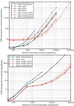
The obtained training times for the different SVM algorithms are displayed in Table 1 and in Figure

7. First, SVMs were trained using standard SVMlightwith the Weighted Degree Kernel precomputed

(WDPre), the standard WD kernel (WD1) and the precomputed (SpecPre) and standard spectrum

kernel (Spec). Then SVMs utilizing thelinaddextension14were trained using the WD (LinWD)

and spectrum (LinSpec) kernel. Finally SVMs were trained on four and eight CPUs using the

parallel version of the linaddalgorithm (LinWD4, LinWD8). WD4 and WD8 demonstrate the

effect of a simple parallelization strategy where the computation of kernel rows and updates on the working set are parallelized, which works with any kernel.

The training times obtained when precomputing the kernel matrix (which includes the time

needed to precompute the full kernel matrix) is lower when no more than 1,000 examples are used.

13. The splice data set can be downloaded fromhttp://www.fml.tuebingen.mpg.de/raetsch/projects/lsmkl. 14. More precisely thelinaddandO(L)block formulation of the WD kernel as proposed in Sonnenburg et al. (2005b)

Note that this is a direct cause of the relatively large subproblem size Q=112. The picture is

different for, say, Q=42 (data not shown) where the WDPre training time is in all cases larger

than the times obtained using the original WD kernel demonstrating the effectiveness of SVMlight’s

kernel cache. The overhead of constructing a trie on Q=112 examples becomes even more visible:

only starting from 50,000 exampleslinaddoptimization becomes more efficient than the original

WD kernel algorithm as the kernel cache cannot hold all kernel elements anymore.15 Thus it would

be appropriate to lower the chunking size Q as can be seen in Table 3.

The linadd formulation outperforms the original WD kernel by a factor of 3.9 on a million

examples. The picture is similar for the spectrum kernel, here speedups of factor 64 on 500,000 examples are reached which stems from the fact that explicit maps (and not tries as in the WD

kernel case) as discussed in Section 3.1.2 could be used leading to a lookupcost of

O

dramatically reduced map construction time. For that reason the parallelization effort benefits the WD kernel more than the Spectrum kernel: on one million examples the parallelization using 4 CPUs (8 CPUs) leads to a speedup of factor 3.25 (5.42) for the WD kernel, but only 1.67 (1.97) for the Spectrum kernel. Thus parallelization will help more if the kernel computation is slow. Training

with the original WD kernel with a sample size of 1,000,000 takes about 28 hours, the linadd

version still requires 7 hours while with the 8 CPU parallel implementation only about 6 hours and

in conjunction with the linadd optimization a single hour and 20 minutes are needed. Finally,

training on 10 million examples takes about 4 days. Note that this data set is already 2.1GB in size.

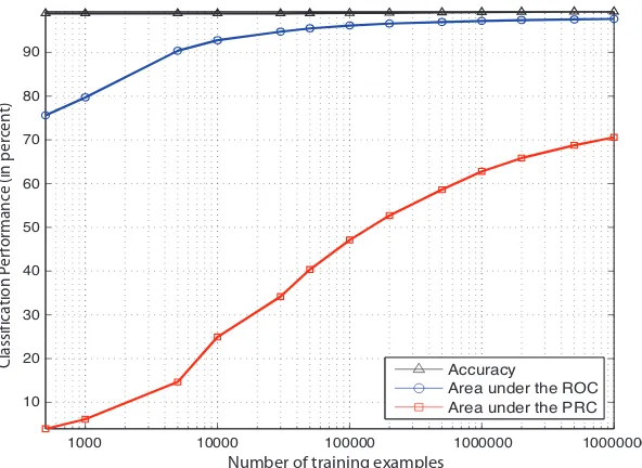
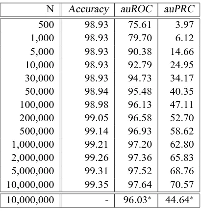
Classification Performance Figure 8 and Table 2 show the classification performance in terms of classification accuracy, area under the Receiver Operator Characteristic (ROC) Curve (Metz, 1978; Fawcett, 2003) and the area under the Precision Recall Curve (PRC) (see e.g. Davis and Goadrich (2006)) of SVMs on the human splice data set for different data set sizes using the WD kernel.

Recall the definition of the ROC and PRC curves: The sensitivity (or recall) is defined as the fraction of correctly classified positive examples among the total number of positive

exam-ples, i.e. it equals the true positive rate T PR=T P/(T P+FN). Analogously, the fraction FPR=

FP/(T N+FP) of negative examples wrongly classified positive is called the false positive rate.

Plotting FPR against TPR results in the Receiver Operator Characteristic Curve (ROC) Metz (1978); Fawcett (2003). Plotting the true positive rate against the positive predictive value (also precision)

PPV=T P/(FP+T P), i.e. the fraction of correct positive predictions among all positively predicted examples, one obtains the Precision Recall Curve (PRC) (see e.g. Davis and Goadrich (2006)). Note that as this is a very unbalanced data set the accuracy and the area under the ROC curve are almost meaningless, since both measures are independent of class ratios. The more sensible auPRC, how-ever, steadily increases as more training examples are used for learning. Thus one should train using all available data to obtain state-of-the-art results.

Varying SVMlight’sqpsizeparameter As discussed in Section 3.1.3 and Algorithm 3, using the

linaddalgorithm for computing the output for all training examples w.r.t. to some working set can

be speed up by a factor of Q (i.e. the size of the quadratic subproblems, termedqpsizein SVMlight).

However, there is a trade-off in choosing Q as solving larger quadratic subproblems is expensive (quadratic to cubic effort). Table 3 shows the dependence of the computing time from Q and N.

For example the gain in speed between choosing Q=12 and Q=42 for 1 million of examples is

54%.Sticking with a mid-range Q (here Q=42) seems to be a good idea for this task. However,

1000 10000 100000 1000000 10000000 100

1000 10000 100000

Number of training examples (logarithmic)

SVM tra

ining tim

e in

seconds (logarithm

ic)

WD−Precompute WD 1CPU WD 4CPU WD 8CPU WD−Linadd 1CPU WD−Linadd 4CPU WD−Linadd 8CPU

1000 10000 100000 1000000 1

10 100 1000 10000

Number of training examples (logarithmic)

SVM training time in seconds (logarithmic)

Spec−Precompute Spec−orig Spec−linadd 1CPU Spec−linadd 4CPU Spec−linadd 8CPU

Figure 7: Comparison of the running time of the different SVM training algorithms using the weighted degree kernel. Note that as this is a log-log plot small appearing distances are large for larger N and that each slope corresponds to a different exponent. In the upper figure the Weighted Degree kernel training times are measured, the lower figure displays Spectrum kernel training times.

a large variance can be observed, as the SVM training time depends to a large extend on which Q variables are selected in each optimization step. For example on the related C. elegans splice data

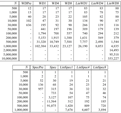
N WDPre WD1 WD4 WD8 LinWD1 LinWD4 LinWD8

500 12 17 17 17 83 83 80

1,000 13 17 17 17 83 78 75

5,000 40 28 23 22 105 82 80

10,000 102 47 31 30 134 90 87

30,000 636 195 92 90 266 139 116

50,000 - 441 197 196 389 179 139

100,000 - 1,794 708 557 740 294 212

200,000 - 5,153 1,915 1,380 1,631 569 379

500,000 - 31,320 10,749 7,588 7,757 2,498 1,544

1,000,000 - 102,384 33,432 23,127 26,190 8,053 4,835

2,000,000 - - - 14,493

5,000,000 - - - 95,518

10,000,000 - - - 353,227

N SpecPre Spec LinSpec1 LinSpec4 LinSpec8

500 1 1 1 1 1

1,000 2 2 1 1 1

5,000 52 30 19 21 21

10,000 136 68 24 23 24

30,000 957 315 36 32 32

50,000 - 733 54 47 46

100,000 - 3,127 107 75 74

200,000 - 11,564 312 192 185

500,000 - 91,075 1,420 809 728

1,000,000 - - 7,676 4,607 3,894

Table 1: (top) Speed Comparison of the original single CPU Weighted Degree Kernel algorithm

(WD1) in SVMlight training, compared to the four (WD4)and eight (WD8) CPUs

par-allelized version, the precomputed version (Pre) and thelinaddextension used in

con-junction with the original WD kernel for 1,4 and 8 CPUs (LinWD1, LinWD4, LinWD8). (bottom) Speed Comparison of the spectrum kernel without (Spec) and withlinadd (Lin-Spec1, LinSpec4, LinSpec8 using 1,4 and 8 processors). SpecPre denotes the precomputed version. The first column shows the sample size N of the data set used in SVM training while the following columns display the time (measured in seconds) needed in the training phase.

1000 10000 100000 1000000 10000000 10

20 30 40 50 60 70 80 90

Number of training examples

Classification

Performance

(in

percent)

Accuracy

Area under the ROC Area under the PRC

Figure 8: Comparison of the classification performance of the Weighted Degree kernel based SVM classifier for different training set sizes. The area under the Receiver Operator Charac-teristic (ROC) Curve, the area under the Precision Recall Curve (PRC) as well as the classification accuracy are displayed (in percent). Note that as this is a very unbalanced data set, the accuracy and the area under the ROC curve are less meaningful than the area under the PRC.

4.2.2 BENCHMARKINGMKL

The WD kernel of degree 20 consist of a weighted sum of 20 sub-kernels each counting matching

d-mers, for d=1, . . . ,20.Using MKL we learned the weighting on the splice site recognition task for

one million examples as displayed in Figure 5 and discussed in Section 4.1.3. Focusing on a speed comparison we now show the obtained training times for the different MKL algorithms applied to learning weightings of the WD kernel on the splice site classification task. To do so, several MKL-SVMs were trained using precomputed kernel matrices (PreMKL), kernel matrices which

are computed on the fly employing kernel caching (MKL16), MKL using the linadd extension

(LinMKL1) andlinaddwith its parallel implementation17(LinMKL4 and LinMKL8 - on 4 and 8

CPUs). The results are displayed in Table 4 and in Figure 9. While precomputing kernel matrices

seems beneficial, it cannot be applied to large scale cases (e.g. >10,000 examples) due to the

O

matrices is computationally extremely demanding, but since kernel caching19 is used, it is still

possible on 50,000 examples in about 57 hours. Note that no WD-kernel specific optimizations are involved here, so one expects a similar result for arbitrary kernels.

16. Algorithm 2.

17. Algorithm 2 with thelinaddextensions including parallelization of Algorithm 4.

18. Using 20 kernels on 10,000 examples requires already 7.5GB, on 30,000 examples 67GB would be required (both using single precision floats).