Experiment Selection for Causal Discovery

Experiment Selection for Causal Discovery

Antti Hyttinen [email protected]

Helsinki Institute for Information Technology Department of Computer Science

P.O. Box 68 (Gustaf H¨allstr¨omin katu 2b) FI-00014 University of Helsinki

Finland

Frederick Eberhardt [email protected]

Philosophy, Division of the Humanities and Social Sciences MC 101-40

California Institute of Technology Pasadena, CA 91125, USA

Patrik O. Hoyer [email protected]

Helsinki Institute for Information Technology Department of Computer Science

P.O. Box 68 (Gustaf H¨allstr¨omin katu 2b) FI-00014 University of Helsinki

Finland

Editor:David Maxwell Chickering

Abstract

Randomized controlled experiments are often described as the most reliable tool available to scien-tists for discovering causal relationships among quantities of interest. However, it is often unclear how many and which different experiments are needed to identify the full (possibly cyclic) causal structure among some given (possibly causally insufficient) set of variables. Recent results in the causal discovery literature have explored various identifiability criteria that depend on the assump-tions one is able to make about the underlying causal process, but these criteria are not directly constructive for selecting the optimal set of experiments. Fortunately, many of the needed construc-tions already exist in the combinatorics literature, albeit under terminology which is unfamiliar to most of the causal discovery community. In this paper we translate the theoretical results and apply them to the concrete problem of experiment selection. For a variety of settings we give explicit constructions of the optimal set of experiments and adapt some of the general combinatorics results to answer questions relating to the problem of experiment selection.

Keywords: causality, randomized experiments, experiment selection, separating systems, com-pletely separating systems, cut-coverings

1. Introduction

of Spirtes et al. (1993) and Pearl (2000), randomized controlled experiments (Fisher, 1935) still often constitute the tool of choice for inferring causal relationships. In the more recent literature on causal discovery, randomized experiments, in combination with novel inference principles, play an increasingly prominent role (Cooper and Yoo, 1999; Tong and Koller, 2001; Murphy, 2001; Eaton and Murphy, 2007; Meganck et al., 2005; Eberhardt et al., 2005; He and Geng, 2008; Hyttinen et al., 2010, 2011; Claassen and Heskes, 2010). Thus, given a set of assumptions one is willing to make in a test setting, questions concerning the optimal choices of the manipulations arise. What sequence of experiments identifies the underlying causal structure most efficiently? Or, given some background knowledge, how can one select an experiment that maximizes (in some to be defined sense) the insight one can expect to gain?

In our work (Eberhardt, 2007; Eberhardt et al., 2010; Hyttinen et al., 2011, 2012a,b) we found that many of these questions concerning the optimal selection of experiments are equivalent to graph-theoretic or combinatoric problems for which, in several cases, there exist solutions in the mathematics literature. Generally these solutions are couched in a terminology that is neither com-mon in the literature on causal discovery, nor obvious for its connections to the problems in causal discovery. The present article is intended to bridge this terminological gap, both to indicate which problems of experiment selection already have formal solutions, and to provide explicit procedures

for the construction of optimal sets of experiments.1 It gives rise to new problems that (to our

knowledge) are still open and may benefit from the exchange of research in causal discovery on the one hand, and the field of combinatorics and graph theory on the other.

2. Causal Models, Experiments, and Identifiability

We consider causal models which represent the relevant causal structure by a directed graphG=

(

V

,

D

), where

V

is the set of variables under consideration, and

D

⊆

V

×

V

is a set of directed

edges among the variables. A directed edge from xi ∈

V

to xj ∈

V

represents a direct causal

influence ofxionxj, with respect to the full set of variables in

V

(Spirtes et al., 1993; Pearl, 2000).

In addition to the graphG, a fully specified causal model also needs to describe the causal processes

that determine the value of each variable given its direct causes. Typically this is achieved either by using conditional probability distributions (in the ‘causal Bayes nets’ framework) or stochastic functional relationships (for ‘structural equation models’ (SEMs)).

In addition to describing the system in its ‘natural’ or ‘passive observational’ state, a causal model also gives a precise definition of how the system behaves under manipulations. Specifically,

consider an intervention that sets (that is, forces) a given variablexi∈

V

to some value randomly

chosen by the experimenter. Such a “surgical” intervention corresponds to deleting all arcs pointing into xi (leaving all outgoing arcs, and any other arcs in the model, unaffected), and disregarding

the specific process by whichxi normally acquires its value.2 The resulting graph is known as the

‘manipulated’ graph corresponding to this intervention. If, in an experiment, the values ofseveral

variables are set by the experimenter, any arcs into any of those variables are deleted. In this way, a

1. The different constructions and bounds presented in the paper are implemented in a code package at:http://www.

cs.helsinki.fi/group/neuroinf/nonparam/.

causal model provides a concrete prediction for the behaviour of the system under any experimental conditions.

The problem of causal discovery is to infer (to the fullest extent possible) the underlying causal model, from sample data generated by the model. The data can come either from a passive obser-vational setting (no manipulations performed by the researcher) or from one or more randomized experiments, each of which (repeatedly) sets some subset of the variables to values determined purely by chance, while simultaneously measuring the remaining variables. We define an

experi-ment

E

= (

J

,

U

)as a partition of the variable set

V

into two mutually exclusive and collectively

exhaustive sets

J

and

U

, where

J

⊆

V

represents the variables that are intervened on (randomized)

in experiment

E

, and

U

=

V

\

J

represents the remaining variables, all of which are passively

ob-served in this experiment. We will not consider the specific distributions employed to randomize the intervened variables, except to require that the distribution is positive over all combinations of values of the intervened variables. Note that the identifiability results mentioned below apply when the variables simultaneously intervened on in one experiment are randomized independently of one another.3

The extent to which the underlying causal model can be inferred then depends not only on the amount of data available (number of samples) but fundamentally also on the details of what experiments are available and what assumptions on the underlying model one can safely make.

In what follows, we only consider modelidentifiability,4that is, we disregard sample size and only

examine the settings under which models can be learned in the large sample limit. The identifiability results we consider build on causal discovery procedures that make one or more of the following standard assumptions on the underlying model:

acyclicity The graphGis often assumed to be acyclic, that is, there exists no directed path from

a node back to itself. This assumption is useful for causal discovery because finding thatx

causesyallows us to deduce thatydoes not causex.

causal sufficiency In many cases only a subset of the variables involved in the underlying data generating process are measured. Even if some variables are unobserved, a causal model

is said to becausally sufficient if there are no unobserved common causes of the observed

variables. Unobserved common causes are typically troublesome because they bring about a dependence between two observed variables that is not due to any actual causal process among the observed variables.

faithfulness Many causal discovery procedures use independence tests as a primary tool for infer-ring the structure of the underlying graph. Such inferences are correct in the limit if the

distri-bution generated by the model isfaithfulto the graph structure, that is, all independencies in

distribution are consequences of the graph structure rather than the specific parameter values defining the quantitative relationships between the variables. Under faithfulness, perturbing the parameters defining the quantitative relationships will not break any of the observed inde-pendencies between the variables in the distribution.

parametric form Some discovery methods rely on the quantitative causal relations between the

variables being restricted to a particular (simple or smooth)parametric form. The most

com-3. For linear cyclic models this assumption can be relaxed; see Lemma 5 in Hyttinen et al. (2012b).

mon such assumption is linearity: the value of each variable is given by a linear sum of the values of its parents plus a stochastic error term.

It is well known that even when one makesallof the above assumptions (using only linearity as a

parametric restriction), the true causal structure is in general underdetermined given only passive observational data, but can be identified using experiments. We can ask more generally: Under

what combination of assumptions and conditions on a set of K experiments{

E

1, . . . ,

E

K} is the

underlying causal structure identified?

If a total of n observed variables is considered, it should come as no surprise that a set of

K =n randomized experiments, each of which intervenes on all but one of the variables, is in

general sufficient to uniquely identify the graphGthat represents the causal structure among then

variables. In each such experiment we can test which of then−1 other variables are direct causes

of the one non-intervened variable. A natural question is whether the full identification ofGcan

be achieved with other sets of experiments, under various combinations of the above assumptions.

In particular, we can ask whether identification can be reached with fewer thannexperiments, or

with experiments that only involve simultaneous interventions on many fewer thann−1 variables

in each experiment.

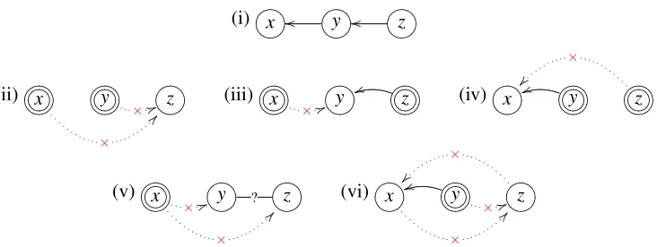
Figure 1 provides an example with three variables. Suppose the true causal structure is the chain x←y←z, as shown in graph (i). Assuming only faithfulnessorlinearity, the three experiments intervening on two variables each are sufficient to uniquely identify the true causal graph. In

par-ticular, when intervening on bothxandy, as illustrated in graph (ii), both of the edges in the true

model are cut, and zis independent of both of the intervened variables, indicating that the edges

x→zandy→zare both absent. On the other hand, when intervening onxandz, as shown in graph

(iii), a dependence is found betweenyandz, indicating thaty←zmust be present, while the

inde-pendence betweenxandyrules out the edgex→y. Similar considerations apply when intervening

on yandz, illustrated in graph (iv). Together, all potential edges in the model are established as either present or absent, and hence the full causal structure is identified. Note that this inference is possible without assuming causal sufficiency or acyclicity.

Assuming causal sufficiency, acyclicity and faithfulness, fewer experiments are needed: If one

had started with an experiment only intervening onx, then a second single intervention experiment

onywould be sufficient for unique identifiability. This is because the first experiment, illustrated in

graph (v), rules out the edgesx→yandx→z, but also establishes, due to the statistical dependence,

thatyandzare connected by an edge (whose orientation is not yet known). Intervening onynext,

as shown in graph (vi), establishes the edgex←y, and the absence of the edgey→z, allowing us

to conclude (using (v)) thaty←zmust be present in the true graph. Finally,xandzare independent

in this second experiment, ruling out the edgex←z. Thus, the true causal structure is identified. If

one had beenluckyto start with an intervention onzthen it turns out that one could have identified

the true causal graph in this single experiment. But that single experiment would, of course, have been insufficient if in fact the causal chain had been oriented in the opposite direction.

The example illustrates the sensitivity of the identifiability results to the model space assump-tions. However, recent research has shown that, in several different settings (described explicitly below), identification hinges on the set of experiments satisfying some relatively simple conditions. Specifically, consider the following conditions:

(i)?>=<89:;x oo ?>=<89:;y oo ?>=<89:;z

(ii)?>=<89:;/.-,()*+x

×

@

@

?>=< 89:;/.-,()*+y

× 55?>=<89:;z (iii)?>=<89:;/.-,()*+x × 55?>=<89:;y ?>=<89:;/.-,()*+z

u

u _{(iv)?>=<89:;x} uu _{?>=<89:;()*+/.-,y ?>=<89:;/.-,()*+z}

×

(v) ?>=<89:;/.-,()*+x

×

@

@

× 55?>=<89:;y ? ?>=<89:;z (vi)?>=<89:;x ×

@

@

?>=< 89:;/.-,()*+y

u

u

× 55?>=<89:;z ×

Figure 1: Graph (i) shows the true data generating structure. Graphs (ii-vi) show the possible infer-ences about the causal structure that can be made from experiments intervening on two variables simultaneously (ii-iv), or intervening on a single variable (v-vi). Variables that are circled twice are intervened on in the corresponding experiment. Edges determined

to be present are solid, edges determined to be absent are dotted and crossed out (×).

The solid line with a question mark denotes an edge determined to be present but whose orientation is unknown. See the text for a description of the background assumptions that support these inferences.

E

k = (

J

k,

U

k)in{

E

1, . . . ,

E

K}such that xi∈

J

k (xi is intervened on) and xj ∈

U

k (xj is passively observed), or xj∈

J

k (xj is intervened on) and xi∈

U

k (xi is passively observed).

Definition 2 (Ordered Pair Condition) A set of experiments {

E

1, . . . ,

E

K} satisfies the ordered pair condition for an ordered pair of variables (xi,xj)∈

V

×

V

(with xi 6=xj) whenever there is an experiment

E

k= (

J

k,

U

k)in{

E

1, . . . ,

E

K}such that xi∈

J

k (xiis intervened on) and xj∈

U

k (xjis passively observed).

Definition 3 (Covariance Condition) A set of experiments {

E

1, . . . ,

E

K} satisfies the covariance condition for an unordered pair of variables{xi,xj} ⊆

V

whenever there is an experiment

E

k=

(

J

k,

U

k) in{

E

1, . . . ,

E

K}such that xi ∈

U

k and xj ∈

U

k, that is, both variables are passively ob-served.

The above conditions have been shown to underlie the following identifiability results: Assuming causal sufficiency, acyclicity and faithfulness, a set of experiments uniquely identifies the causal

structure of a causal Bayes net if and only if for any two variables xi,xj ∈

V

one of the

follow-ing is true: (i) the ordered pair condition holds for the ordered pairs(xi,xj)and(xj,xi), or (ii) the

unordered pair condition and the covariance condition hold for the unordered pair {xi,xj}

(Eber-hardt, 2007). Note that the ‘only if’ part is a worst-case result: For any set of experiments that does not satisfy the above requirement, there exists a causal graph such that the structure is not

identified with these experiments. Since a single passive observation—a so-callednull-experiment,

as

J

=/0—satisfies the covariance condition for all pairs of variables, under the stated assumptions

the main challenge is to find experiments that satisfy theunordered pair conditionfor every pair of

Without causal sufficiency, acyclicity or faithfulness, but assuming a linear data generating

model, a set of experiments uniquely identifies5the causal structure among the observed variables

of a linear SEM if and only if it satisfies theordered pair conditionfor all ordered pairs of variables

(Eberhardt et al., 2010; Hyttinen et al., 2010, 2012a,b). Similar identifiability results can be ob-tained for (acyclic) causal models with binary variables by assuming a noisy-OR parameterization for the local conditional probability distributions (Hyttinen et al., 2011).

Such identifiability results immediately give rise to the following questions of optimal experi-ment selection:

• What is the least number of experiments that satisfy the above conditions?

• Can we give procedures to construct such sets of experiments?

The above questions can be raised similarly given additional context, such as the following:

• The number of variables that can be subject to an intervention simultaneously is limited in

some way.

• Background knowledge about the underlying causal structure is available.

Naturally, there are other possible scenarios, but we focus on these, since we are aware of their counterparts in the combinatorics literature. To avoid having to repeatedly state the relevant search space assumptions, we will present the remainder of this article in terms of the satisfaction of the (unordered and ordered) pair conditions, which provide the basis for the identifiability results just cited.

3. Correspondence to Separating Systems and Cut-coverings

The satisfaction of the pair conditions introduced in the previous section is closely related to two

problems in combinatorics: Finding (completely) separating systems, and finding (directed)

cut-coverings. Throughout, to simplify notation and emphasize the connections, we will overload sym-bols to the extent that there is a correspondence to the problem of experiment selection for causal discovery.

Definition 4 (Separating System) Aseparating system

C

={

J

1,

J

2, . . . ,

J

K}is a set of subsets of an n-set

V

with the property that given any two distinct elements xi,xj∈

V

, there exists a

J

k∈

C

such that xi∈

J

k∧xj∈/

J

korxi∈/

J

k∧xj∈

J

k.

Definition 5 (Completely Separating System) Acompletely separating system

C

={

J

1,

J

2, . . . ,

J

K} is a set of subsets of an n-set

V

with the property that given any two distinct elements xi,xj∈

V

, there exist

J

k,

J

k′∈

C

such that x_i∈

J

_k∧x_j ∈/

J

_k andx_i∈/

J

_k′∧x_j∈

J

_k′.

As can be easily verified, a set of experiments{

E

1, . . . ,

E

K}that satisfies theunorderedpair

condi-tion for all pairs overnvariables in

V

directly corresponds to a separating system over the variable

set, while a set of experiments that satisfies theorderedpair condition for all ordered variable pairs

corresponds to acompletelyseparating system over the variables.6

A related but more general problem is that of finding cut-coverings. First, we need to define

cuts and directed cuts: Acut

E

k corresponds to a partition of a set of vertices

V

of an undirected

graphH= (

V

,

P

)into two sets

J

and

U

. Any edgep∈

P

connecting anxi∈

J

to anxu∈

U

is said

to bein the cut

E

k. For a directed graphF, adirected cutis a cut where only the edgesfromvertices

in

J

tovertices in

U

are in the cut, while edges in the opposite direction are not. We are thus ready

to define acut-coveringand adirected cut-covering:

Definition 6 (Cut-covering) A cut-covering for an undirected graph H = (

V

,

P

)is a set of cuts {

E

1, . . . ,

E

K}such that each edge p∈

P

of H is in some cut

E

k.

Definition 7 (Directed Cut-covering) A directed cut-covering for a directed graph F= (

V

,

Q

)is a set of directed cuts{

E

1, . . . ,

E

K}such that each directed edge q∈

Q

of F is in some directed cut

E

k.

The correspondence of finding cut-coverings to the problem of experiment selection is now immediate: In the case of searching for a set of experiments that satisfies the ordered pair condition

for all ordered pairs of variables in

V

, let the graph F = (

V

,

Q

) be a complete directed graph

over the vertex set

V

where each ordered pair of variables is connected by a directed edge. Each

directed edge represents an ordered pair condition for a pair of vertices (xi,xj) that needs to be

satisfied by the set of experiments. Finding such a set of experiments is then equivalent to finding

a directed cut-covering forF, where each experiment corresponds to a directed cut. An analogous

correspondence holds for the unordered pair condition with a complete undirected graphH. We

discuss the generalization and interpretation of the problem whenH orF are not complete graphs

in Section 6.

As our overloading of symbols suggests, most aspects of the experiment selection have direct counterparts in the cut-covering representation. However, the edges representing direct causes in

a causal graphG do not correspond to the edges representing the satisfaction of an ordered pair

condition in the directed graphF. That is,FandGin general do not share the same edge structure:

Gis the graph of the underlying causal model to be identified, whileFrepresents the set of ordered

pairs that are not yet satisfied. Moreover, there is a difference in how the causal graphGis changed

in light of an experiment

E

= (

J

,

U

), and how the ordered pair graphF is changed in light of the

(corresponding) cut

E

. The experiment

E

results in the manipulated causal graph G′, which is

the same as the original causal graphGexcept that the edgesintothe variables in

J

are removed.

The corresponding cut

E

, however, cuts the edges of the ordered pair condition graph F that are

outgoingfrom variables in

J

(and simultaneouslyintovariables in

U

). This may seem unintuitive,

but in fact these two representations of

E

(the experiment and the cut) illustrate two aspects of what

an experiment achieves: It manipulates the underlying causal graphG(by breaking incoming edges

on variables in

J

), and it satisfies the ordered pair condition for all ordered pairs(xj,xu)withxj∈

J

andxu∈

U

by determining whetherxj has a causal effect onxu. Similarly in the unordered case,

the causal graphG(or its skeleton) must not be confused with the undirected graphHrepresenting

the unordered pairs that are not yet satisfied.

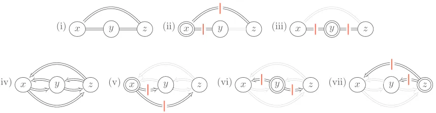
Figure 2: Top: Satisfaction of the unordered pair condition for all pairs of variables in a three variable model. Undirected double-lined edges indicate pairs for which the unordered

pair condition needs to be satisfied (graph (i)). The cuts (|) indicate which pairs are

satisfied by the experiments intervening on x (graph (ii)) and y (graph (iii)). Bottom:

Satisfication of the ordered pair condition: Directed double-lined edges indicate ordered pairs for which the ordered pair condition needs to be satisfied (graph (iv)). Graphs (v-vii) show which pairs are in the directed cuts (are satisfied) by the respective single-intervention experiments. See text for details.

Figure 2 illustrates for a three variable model (such as that in Figure 1) how the satisfaction of the (un)ordered pair condition for all pairs of variables is guaranteed using cut-coverings. Graph (i)

gives the completeundirectedgraphHover{x,y,z}illustrating the three unordered pairs for which

theunordered pair condition needs to be satisfied. Graphs (ii) and (iii) show for which pairs the

unordered pair condition is satisfied by a single intervention experiment onx(ory, respectively), that

is, which pairs are in the cut (|). The pairs that remain unsatisfied by each experiment, respectively,

are shown in gray for easier legibility. Together these experiments constitute a cut-covering forH.

Similarly, graph (iv) gives the completedirectedgraphFover the three variables, illustrating the six

ordered pairs of variables for which theorderedpair condition needs to be satisfied. Graphs (v-vii)

show for which pairs the ordered pair condition is satisfied by a single intervention experiment on x(oryorz, respectively), that is which pairs are in the directed cut (|), while the others are again shown in gray. As can be seen, in the ordered case all three experiments are needed to provide a

directed cut-covering forF.

The correspondence between the problem of finding experiments that satisfy the pair conditions on the one hand and finding separating systems or cut-coverings on the other, allows us to tap into the results in combinatorics to inform the selection of experiments in the causal discovery problem.

4. Minimal Sets of Experiments

I

1 = {}

I

2 = {1}

I

3 = {2}

I

4 = {1,2}

I

5 = {3}

I

6 = {1,3}

I

7 = {2,3}

−→

J

3

J

2

J

1

I

1 0 0 0

I

2 0 0 1

I

3 0 1 0

I

4 0 1 1

I

5 1 0 0

I

6 1 0 1

I

7 1 1 0

−→

J

1={x2,x4,x6}

J

2={x3,x4,x7}

J

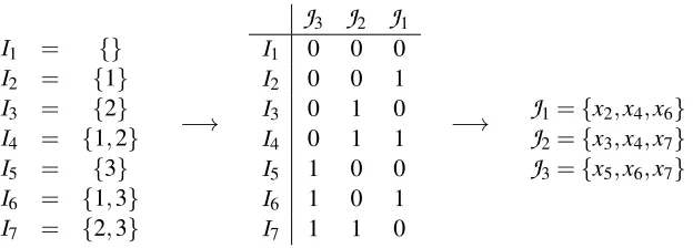
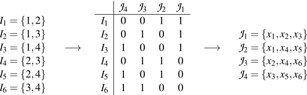
3={x5,x6,x7}

Figure 3: An illustration of the relationship between intervention sets and index sets, giving the

construction of a minimal set of experiments satisfying theunorderedpair condition for

all pairs of variables in a 7 variable model. The index sets

I

1, . . . ,

I

n (left) are chosen

as distinct subsets of the set of experiment indexes{1,2,3}, and each row of the binary

matrix (middle) marks the corresponding experiments. The intervention sets

J

1, . . . ,

J

K

(right) are then obtained by reading off the columns of this matrix. Note that one ad-ditional variable could still be added (intervened on in all three experiments) while still satisfying the unordered pair condition for all variable pairs. For nine variables, however, a minimum of four experiments would be needed.

implemented in our associated code package. Throughout,i=1, . . . ,nindexes the variables in the

variable set

V

, whilek=1, . . . ,Kindexes the experiments in the construction.

Many of the constructions of intervention sets

J

1, . . . ,

J

Kwill be examined using so-calledindex sets

I

1, . . . ,

I

n, where

I

i = {k|xi∈

J

k}.

That is, thei:th index set simply lists the indexes of the intervention sets that include the variable

xi. Clearly,Kexperiments (or separating sets) overnvariables can be defined either in terms of the

intervention sets

J

1, . . . ,

J

K or equivalently in terms of the index sets

I

1, . . . ,

I

n. See Figure 3 for an illustration.

4.1 Satisfying the Unordered Pair Condition

The earliest results (that we are aware of) relevant to finding minimal sets of experiments satisfying

the unordered pair condition are given in R´enyi (1961)7in the terminology of separating systems.

He found that a separating system

C

={

J

1,

J

2, . . . ,

J

K}over

V

can be obtained by assigning distinct

binary numbers to each variable in

V

. That is, the strategy is to choose distinct index sets for all

variables in

V

. This is supported by the following Lemma:

Lemma 8 (Index sets must be distinct) Intervention sets {

J

1, . . . ,

J

K} satisfy the unordered pair condition for all unordered pairs of variables if and only if the corresponding index sets

I

1, . . . ,

I

n are distinct.

Proof Assume that the index sets are distinct. Since the index sets

I

i and

I

j of any two variables are distinct, there must exist an indexksuch that eitherk∈

I

iandk∈/

I

j, ork∈/

I

iandk∈

I

j. Thus, the experiment

E

ksatisfies the unordered pair condition for the pair{xi,xj}.

Next assume that the unordered pair condition is satisfied for all pairs. Take two arbitrary index sets

I

i and

I

j. Since the unordered pair condition is satisfied for the pair{xi,xj}, there is an

experiment

E

k wherexi is intervened on andxj is not, orxj is intervened andxiis not. Either way,

I

i6=

I

j.

Again, Figure 3 is used to illustrate this concept.

R´enyi (1961, p. 76) notes that the smallest separating system for a set ofnvariables has size

c(n) = ⌈log₂(n)⌉. (1)

This is clear from the previous lemma: K experiments only allow for up to 2K distinct index sets.

Equivalent results and procedures are derived, only in the terminology of finding minimal cut-coverings for complete graphs, by Loulou (1992, p. 303). In the terminology of causal discovery,

Eberhardt (2007, Theorem 3.3.4) requires⌊log₂(n)⌋+1 experiments to guarantee identifiability of

a causal model.8 For graphs over three variables, the result is obvious given the graphH (for the

unordered pair condition) in Figure 2 (top, left): For a cut-covering of the three undirected edges,

2=⌈log₂(3)⌉cuts are necessary and sufficient. The two cuts in graphs (ii) and (iii) in Figure 2

corresponding to the experiments in the last row of Figure 1 are an example. Figure 4 shows the number of experiments needed to satisfy the unordered pair condition for all variable pairs for models of up to 5,000 variables.

4.2 Satisfying the Ordered Pair Condition

When Dickson (1969, p. 192) coined the term “completely separating systems”, he also showed

that as the numbern=|

V

|of elements tends to infinity, the size of a minimal completely separating

system approaches the size of a (standard) separating system, that is, log₂(n). However, Dickson did

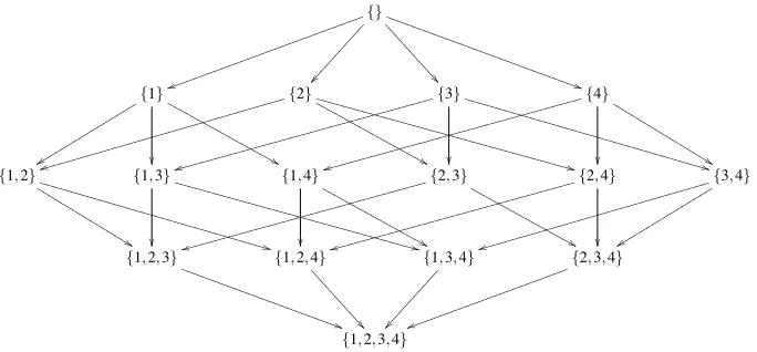
not derive the exact minimal size. Shortly after, Spencer (1970) recognized the connection between completely separating systems and antichains in the subset lattice, as defined below. See Figure 5 for an illustration.

Definition 9 (Antichain) An antichain (also known as a Sperner system){

S

i} over a set

S

is a family of subsets of

S

such that∀i,j:

S

i*

S

j and

S

i+

S

j.

The connection between antichains and completely separating systems (that is, satisfying the or-dered pair condition) is then the following:

Lemma 10 (Index sets form an antichain) The intervention sets{

J

1, . . . ,

J

K} satisfy the ordered pair condition for all ordered pairs if and only if the corresponding index sets{

I

1, . . . ,

I

n}form an antichain over{1, . . . ,K}.

8. The one additional experiment sometimes required in this case derives from the need to satisfy the ordered pair condition, or unordered pair conditionandthe covariance condition, for each pair of variables, as discussed in Sec-tion 2. The covariance condiSec-tion can be trivially satisfied with a single passive observaSec-tional data set (a so-called

Figure 4: Sufficient and necessary number of experiments needed to satisfy the unordered (blue, lower solid line) and the ordered (red, upper solid line) pair condition for models of different sizes (in log-scale). The number of variables in the models are only ticked on the x-axis when an additional experiment is needed. For example, for a model with 100 variables, 7 experiments are needed to satisfy the unordered pair condition, while 9 experiments are needed to satisfy the ordered pair condition.

{} u u ❦❦❦❦❦❦ ❦❦❦❦❦❦ ❦❦❦❦❦❦ ❦❦❦❦❦❦ ❦❦❦❦❦ ✂✂✂✂ ✂✂✂✂ ✂✂✂ ❁ ❁ ❁ ❁ ❁ ❁ ❁ ❁ ❁ ❁ ❁ ) ) ❙ ❙ ❙ ❙ ❙ ❙ ❙ ❙ ❙ ❙ ❙ ❙ ❙ ❙ ❙ ❙ ❙ ❙ ❙ ❙ ❙ ❙ ❙ ❙ ❙ ❙ ❙ ❙ ❙

{1}

y y rrrr rrrr rrrr rrrr

▼▼▼▼&& ▼ ▼ ▼ ▼ ▼ ▼ ▼ ▼ ▼ ▼ ▼ ▼ ▼

▼ {2}

t t ❤❤❤❤❤❤❤❤❤ ❤❤❤❤❤❤❤❤❤ ❤❤❤❤❤❤❤❤❤ ❤❤❤❤❤❤❤❤❤ & & ▼ ▼ ▼ ▼ ▼ ▼ ▼ ▼ ▼ ▼ ▼ ▼ ▼ ▼ ▼ ▼ ▼ ▼ + + ❱ ❱ ❱ ❱ ❱ ❱ ❱ ❱ ❱ ❱ ❱ ❱ ❱ ❱ ❱ ❱ ❱ ❱ ❱ ❱ ❱ ❱ ❱ ❱ ❱ ❱ ❱ ❱ ❱ ❱ ❱ ❱ ❱ ❱ ❱ ❱ ❱

❱ {3}

s s ❤❤❤❤❤❤❤ ❤❤❤❤❤❤❤❤ ❤❤❤❤❤❤❤❤ ❤❤❤❤❤❤❤❤ ❤❤❤❤❤❤❤

❱❱❱❱❱❱❱❱❱❱❱❱❱❱❱❱❱❱{❱❱4❱}❱❱❱❱❱❱❱❱❱❱❱❱❱❱❱**

s s ❤❤❤❤❤❤❤ ❤❤❤❤❤❤❤❤ ❤❤❤❤❤❤❤❤ ❤❤❤❤❤❤❤❤ ❤❤❤❤❤❤❤ ▲▲▲▲▲%% ▲ ▲ ▲ ▲ ▲ ▲ ▲ ▲ ▲ ▲ ▲

{1,2}

% % ▲ ▲ ▲ ▲ ▲ ▲ ▲ ▲ ▲ ▲ ▲ ▲ ▲ ▲ ▲ ▲ * * ❱ ❱ ❱ ❱ ❱ ❱ ❱ ❱ ❱ ❱ ❱ ❱ ❱ ❱ ❱ ❱ ❱ ❱ ❱ ❱ ❱ ❱ ❱ ❱ ❱ ❱ ❱ ❱ ❱ ❱ ❱ ❱ ❱

❱ {1,3}

❱❱❱❱❱❱❱❱❱❱❱❱❱❱❱❱{❱❱1❱,❱4}❱❱❱❱❱❱❱❱❱❱❱❱❱❱❱❱++

▼▼▼▼▼▼&& ▼ ▼ ▼ ▼ ▼ ▼ ▼ ▼ ▼ ▼

▼ {2,3}

s s ❤❤❤❤❤❤❤❤ ❤❤❤❤❤❤❤❤ ❤❤❤❤❤❤❤❤ ❤❤❤❤❤❤❤❤ ❤❤❤❤ & & ▼ ▼ ▼ ▼ ▼ ▼ ▼ ▼ ▼ ▼ ▼ ▼ ▼ ▼ ▼ ▼

▼ {2,4}

s s ❤❤❤❤❤❤❤❤ ❤❤❤❤❤❤❤❤ ❤❤❤❤❤❤❤❤ ❤❤❤❤❤❤❤❤ ❤❤❤❤

{3,4}

t t ❤❤❤❤❤❤❤❤❤ ❤❤❤❤❤❤❤❤❤ ❤❤❤❤❤❤❤❤❤ ❤❤❤❤❤❤❤ y y rrrr rrrr rrrr rrrr

{1,2,3}

) ) ❙ ❙ ❙ ❙ ❙ ❙ ❙ ❙ ❙ ❙ ❙ ❙ ❙ ❙ ❙ ❙ ❙ ❙ ❙ ❙ ❙ ❙ ❙

❙ {1,2,4}

❁ ❁ ❁ ❁ ❁ ❁ ❁ ❁ ❁ ❁

❁ {1,3,4}

✂✂✂✂ ✂✂✂✂

✂✂✂

{2,3,4}

u u ❦❦❦❦❦❦ ❦❦❦❦❦❦ ❦❦❦❦❦❦ ❦❦❦❦❦❦

{1,2,3,4}

Figure 5: Subset lattice of subsets of{1,2,3,4}. A directed path from set

S

ito set

S

j exists if and

only if

S

i⊂

S

j. The largest antichain is the family of sets that are not connected by any

I

1={1,2}

I

2={1,3}

I

3={1,4}

I

4={2,3}

I

5={2,4}

I

6={3,4}

−→

J

4

J

3

J

2

J

1

I

1 0 0 1 1

I

2 0 1 0 1

I

3 1 0 0 1

I

4 0 1 1 0

I

5 1 0 1 0

I

6 1 1 0 0

−→

J

1={x1,x2,x3}

J

2={x1,x4,x5}

J

3={x2,x4,x6}

J

4={x3,x5,x6}

Figure 6: Designing the intervention sets of experiments satisfying theorderedpair condition for

all ordered pairs of variables in an=6 variable model withK=4 experiments. Select

the index sets

I

1, . . . ,

I

nas an antichain over{1, . . . ,K}and translate the index sets into intervention sets

J

1, . . . ,

J

K.

Proof Assume that the index sets form an antichain. Consider an arbitrary ordered pair(xi,xj).

Since index sets form an antichain we have that

I

i*

I

j and there must be experiment

E

k such that

k∈

I

iandk∈/

I

j. This experiment satisfies the ordered pair condition for the ordered pair(xi,xj). Next assume that the ordered pair condition is satisfied for all ordered pairs. Take two arbitrary index sets

I

i and

I

j. Since the ordered pair condition is satisfied for the pair (xi,xj), there is an

experiment wherexi is intervened on andxj is not, thus

I

i*

I

j. Symmetrically,

I

j*

I

i. Thus the

index sets form an antichain.

Earlier, Sperner (1928) had already proven the following theorem on the maximum possible size of an antichain.

Theorem 11 (Sperner’s Theorem) The largest antichain over{1, . . . ,K}is formed by the subsets of constant size⌊K/2⌋and thus has size _⌊KK_/2⌋.

Thus, the minimal completely separating system over a set of sizencan always be constructed

by selecting the corresponding index sets as any distinct ⌊K/2⌋-size subsets. See Figure 6 for

an illustration. Using this rationale, Spencer (1970) notes that the cardinalityc(n) of a minimal

completely separating system fornelements is given by

c(n) = min{K:

K ⌊K/2⌋

≥n}, (2)

which can be approximated using Stirling’s approximation as

c(n) =log₂(n) +1

2log2log2(n) + 1 2log2(

π

2) +o(1).

Equation 2 is re-proven for directed cut-coverings over complete graphs by Alon et al. (2007, The-orem 11), also using the connection to antichains. To our knowledge, tight bounds or constructions have not been previously described in the causal discovery literature on experiment selection.

For graphs over three variables, the graphF(for the ordered pair condition) in Figure 2 (bottom,

double-intervention experiments in graphs (ii-iv) of Figure 1 would also work. Figure 4 shows the

number of experiments required for models with up to 5,000 variables. Note that the difference

between the number of experiments needed for a separating and a completely separating system over a given number of variables is only 2 or 3 experiments. Thus, in many cases the possibility of applying an inference procedure based on weaker assumptions may be worth the investigative cost of a few additional experiments to satisfy the ordered pair condition.

5. Limiting Intervention Set Size

Section 4 focused on characterizing minimal sets of experiments that guarantee identifiability, but paid no attention to the particular nature of those experiments. In some cases, the experiments might require a simultaneous intervention on half of the variables, but of course such experiments will in many scientific contexts not be feasible. In this section we consider a generalization of the problem of finding the optimal set of experiments that can take into account additional constraints on the size of the intervention sets. We consider the following variants of the problem:

1. Given n variables and K experiments, find intervention sets

J

1, . . . ,

J

K ⊆

V

satisfying the

ordered or unordered pair condition for all variable pairs, such that the intervention sets have minimal

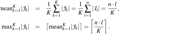
(a) averageintervention set size meanK_k=1|

J

k|=_K1∑Kk=1|

J

k|(which is equivalent to mini-mizing the total number of interventions), or

(b) maximumintervention set size maxK_k=1|

J

k|.

2. Givennvariables and a maximum allowed intervention set sizer, find the minimum number

of experimentsm(n,r)for which there exists intervention sets

J

1, . . . ,

J

m(n,r)⊆

V

that satisfy

the ordered or unordered pair condition for all variable pairs.

As will become clear from the following discussion, these problems are related. Note that, de-pending on the additional constraints, these problems may not have solutions (for example, for the

unordered case of Problem 1(a) and 1(b), whenKis smaller than the bound given in Equation 1), or

they may trivially reduce to the problems of the previous sections because the additional constraints are irrelevant (for example, Problem 2 reduces for the unordered case to the problem discussed in

Section 4.1 ifr≥n/2). As in the previous section, we separate the discussion of the results into

those pertaining to theunordered pair condition (Section 5.1) and those pertaining to theordered

pair condition (Section 5.2). The algorithms presented here can also be used to construct interven-tion sets that satisfy the bounds discussed in Secinterven-tion 4.

5.1 Limiting the Intervention Set Size for the Unordered Pair Condition

We start with the simplest problem, Problem 1(a) for theunorderedcase, and give the construction

of a set of experiments that achieves the smallest possibleaverageintervention set size, given the

number of variables n and the number of experiments K. The construction we present here is

I

1 = {}

I

2 = {1}

I

3 = {2}

I

4 = {3}

I

5 = {4}

I

6 = {1,2}

I

7 = {3,4}

−→

J

4

J

3

J

2

J

1

I

1 0 0 0 0

I

2 0 0 0 1

I

3 0 0 1 0

I

4 0 1 0 0

I

5 1 0 0 0

I

6 0 0 1 1

I

7 1 1 0 0

−→

J

1={x2,x6}

J

2={x3,x6}

J

3={x4,x7}

J

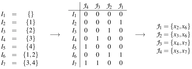
4={x5,x7}

Figure 7: Intervention sets for experiments that satisfy theunorderedpair condition for all pairs of

variables in a 7 variable model such that both the maximum and average intervention set size are minimized. The index sets were chosen using Algorithm 2.

set sizes (because both represent the total number of interventions):

K

∑

k=1

|

J

k| = n

∑

i=1

|

I

i|. (3)

This identity, together with Lemma 8, implies that to obtain intervention sets with minimum average size, it is sufficient to find thensmallest distinct subsets of{1, . . . ,K}as the index sets. There are a total of∑p_j=0 K_jindex sets

I

iwith|

I

i| ≤p. Consequently, the sizelof the largest required index set is the integer solution to the inequalities

l−1

∑

j=0

K j

< n ≤

l

∑

j=0

K j

. (4)

If there is no solution forl, the unordered pair condition cannot be satisfied withKexperiments. If

there is a solution, the inequalities in Equation 4 imply that when choosing the smallest index sets,

we have to selectall

t =

l−1

∑

j=0

K j

index sets of sizes 0 tol−1, and the remainingn−tsets of sizel. Since the sum of the intervention

set sizes is the same as the sum of the index set sizes (Equation 3), the average intervention set size obtained is

meanK_k=1|

J

k| = 1 K

K

∑

k=1 |

J

k| =

1 K

n

∑

i=1 |

I

i| =

1 K

"

l−1

∑

j=0 j

K j

+l(n−t) #

. (5)

ForK experiments this is the minimum average intervention set size possible that satisfies the

un-ordered pair condition for all pairs amongnvariables. For the case ofn=7 variables and K=4

experiments, Figure 7 provides an example of the construction of intervention sets with minimal

av-erage size. Note that the minimum avav-erage would not have been affected if the index sets

I

6and

I

7

Algorithm 1Selectspindex sets of sizel, forKexperiments, such that the indexes are distributed fairly among the index sets. The idea of this algorithm appears in a proof in Cameron (1994, accredited to D. Billington).

Fair(K,l,p)

Draw the index sets{I1, . . . ,Ip}as distinctl-size subsets of{1, . . . ,K}.

WhileTRUE,

Find the most frequent indexMand the least frequent indexmamong the index sets{I1, . . . ,Ip}.

Iffreq(M)−freq(m)≤1then exit the loop.

Find10a setAof sizel−1such that({M} ∪A)∈ {I1, . . . ,Ip}and({m} ∪A)∈ {/ I1, . . . ,Ip}.

Replace the index set({M} ∪A)with({m} ∪A)in{I1, . . . ,Ip}.

Return the index sets{I1, . . . ,Ip}.

The minimum average intervention set size in Equation 5 also gives a lower bound for the

lowest possiblemaximumintervention set size, given the number of experimentsK and variables

n(Problem 1(b)): At least one intervention set of size⌈meanK_k=1|

J

k|⌉or larger is needed, because otherwise the intervention sets would yield a lower average. Next, we will show that this is also an upper bound.

The size of an arbitrary intervention set

J

k is equal to the number of index sets that contain the

indexk. We say that index sets are selectedfairlywhen the corresponding intervention sets satisfy

|

J

k| − |

J

k′| ≤ 1 ∀k,k′. (6)

In the construction that minimizes the average intervention set size, the index sets

I

1, . . . ,

I

t

constituteallpossible subsets of{1, . . . ,K}of sizel−1 or less, and consequently all indexes appear

equally often in these sets.9 The remainingn−tindex sets can be chosenfairlyusing Algorithm 1.

It finds fair index sets by simply switching the sets until the experiment indexes appear fairly. Since (i) the average intervention set size remains unchanged by this switching, (ii) the minimum average constitutes a lower bound, and (iii) the intervention set sizes differ by at most one, it follows (see Appendix A) that the lowest maximum intervention set size is given by

maxK_k=1|

J

k| = ⌈meanKk=1|

J

k|⌉. (7)

Thus, if the construction of index sets isfair, thenboththe minimum average and the smallest

maximum intervention set size is achieved, simultaneously solving both Problem 1(a) and 1(b). Algorithm 2 provides this complete procedure. Note that in general it is possible to select index sets such that the maximum intervention set size is not minimized, even though the average is minimal

(for example, if

I

7 had been{1,4}in Figure 7). Figure 8 (top) shows the lowest possible average

intervention set sizes. Rounding these figures up to the closest integer gives the lowest possible

9. This is easily seen if the index sets are represented as binary numbers, as in the center of Figure 7. It is also clear from considerations of symmetry.

Algorithm 2ConstructsK intervention sets that satisfy the unordered pair condition for all pairs

amongnvariables with a minimum average and smallest maximum intervention set size.

FairUnordered(n,K)

Determine the maximum index set size l from Equation 4, if no such l exists, then the unordered pair

condition cannot be satisfied fornvariables withKexperiments.

Assign all subsetsS⊆ {1, . . . ,K}such that|S| ≤l−1to index setsI1, . . . ,It.

Draw the remainingl-size index sets with: It+1, . . . ,In←Fair(K,l,n−t)

Return the intervention setsJ1, . . . ,JKcorresponding to the index setsI1, . . . ,In.

Algorithm 3ConstructsK intervention sets that satisfy theorderedpair condition for all ordered

pairs among n variables and approximates (and sometimes achieves) the minimum average and

smallest maximum intervention size.

FairOrdered(n,K)

Determine the maximum index set sizelfrom Equation 10, if no suchlexists, then the ordered pair condition

cannot be satisfied fornvariables withKexperiments.

Draw thel-size index sets with: I1, . . . ,In←Fair(K,l,n)

Return the intervention setsJ1, . . . ,JKcorresponding to the index setsI1, . . . ,In.

maximum intervention set sizes. All of these numbers are achieved by intervention sets constructed using Algorithm 2.

Using constructions similar to the above, Katona (1966) and Wegener (1979) were able to derive

the following bounds for Problem 2, the minimum number of experimentsm(n,r) given an upper

boundron the intervention set sizes:

m(n,r) = ⌈log₂n⌉, ifr>n/2, (8) log₂n

log₂(e·n/r) n

r ≤ m(n,r) ≤

log₂n log₂⌈n/r⌉

(⌈n/r⌉ −1), ifr≤n/2, (9)

where e denotes Euler’s number. Equation 8 just restates Equation 1, since the constructions in

Section 4.1 without a constraint on the maximum intervention set size result in intervention sets

with no more thann/2 variables. For any practical values ofn andr, the value of m(n,r) can be

found by simply evaluating Equations 4, 5 and 7 for different values ofK (starting from the lower

bound in 9), so as to find the smallest value ofK for which the maximum intervention set size is

smaller than or equal tor. Figure 8 (bottom) illustrates the behavior of the functionm(n,r)and the

bounds given by Equation 9.

5.2 Limiting the Intervention Set Size for the Ordered Pair Condition

Recall from Lemma 10 that satisfaction of theorderedpair condition requires that then index sets

of a set of K experiments form an antichain over {1, . . . ,K}. Thus, no matter whether we seek

to minimize the average or the maximum intervention set size, we have to ensure that the index

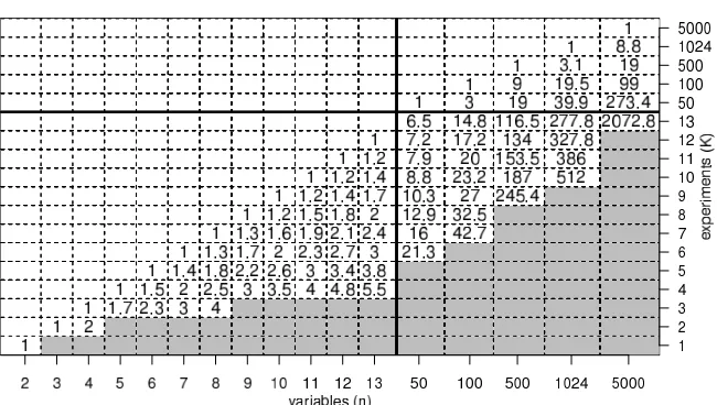
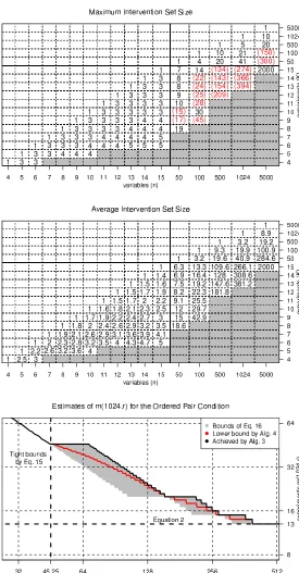
Figure 8: Satisfying the unordered pair condition while limiting the intervention set sizes. Top:

Lowest achievable average intervention set sizes for models with n variables using K

experiments. The lowest achievable maximum intervention set size is the ceiling of the average intervention set size shown in the figure. Grey areas denote an insufficient num-ber of experiments to satisfy the unordered pair condition. Blank areas are uninteresting, since the average intervention set size can be lowered here by including irrelevant

pas-sive observational (null-)experiments. Bottom: The number of experiments needed for

1(b): GivennandK, we want to specify experiments minimizing either the average or maximum intervention set size.

First, we note that to obtain an antichain with nelements fromK experiments, at least one of

the index sets must be of cardinalitylor larger, wherelis chosen to satisfy

K l−1

< n ≤

K l

. (10)

This must be the case because it can be shown using the Lemmas in the proof of Theorem 11 (see

p. 546 bottom in Sperner, 1928) that the largest antichain with sets of at most sizel−1 has size

K l−1

, which—given how lwas constructed in Equation 10—is not enough to accommodate alln

index sets. On the other hand, it is equally clear that itispossible to obtain an antichain by selecting

thenindex sets to all have sizesl.

Thus, a simple approach to attempt to minimize the maximum intervention set size (that is,

solve Problem 1 (b)) is to select thenindex sets all with sizes land use Algorithm 3, exploiting

Algorithm 1, to construct afairset of index sets. This construction is not fully optimal in all cases

because all sets are chosen with sizel while in some cases a smaller maximum intervention set

size is achievable by combining index sets of different sizes. It is easily seen that Algorithm 3 will generate sets of experiments that have an average and a maximum intervention set size of

meanK_k=1|

J

k| = 1 K

K

∑

k=1 |

J

k|=

1 K

n

∑

i=1 |

I

i|=

n·l

K , (11)

maxK_k=1|

J

k| =

meanK_k=1|

J

k|

=

n·l K

. (12)

Figure 9 (top) shows the maximum intervention set size in the output of Algorithm 3 for several

values ofnandK. Given some of the subsequent results it can also be shown that some of these are

guaranteed to be optimal.11 While this scheme for solving the directed case of Problem 1(b) is quite

good in practice, we are not aware of any efficient scheme that is always guaranteed to minimize the maximum intervention set size.

Alternatively, one may focus on Problem 1 (a) and thus attempt to minimize the average

in-tervention set size. For this problem, there exists an efficient procedure that obtains the optimum. Griggs et al. (2012) have recently provided some results in this direction. Here we apply their find-ings to the problem of experiment selection. To present the construction we need to start with some results pertaining to antichains.

An antichain is said to beflatif for any pair of sets

I

i and

I

j in the antichain, the cardinalities satisfy

|

I

i| − |

I

j| ≤1, ∀i,j.

Note thatflatnessrequires a selection of index sets that arethemselvesclose in size, whilefairness

(Equation 6) requires a selection of index sets such that theintervention setsare close in size. Using

this notion of flatness, Lieby (1994) originally formulated the following theorem as a conjecture:

Figure 9: Satisfying the ordered pair condition while limiting the size of the intervention sets.Top: Maximum intervention set sizes achieved by Algorithm 3. Black numbers mark the cases where the achieved maximum intervention set size is known to be optimal, while red

numbers in parentheses mark cases that are not known to be optimal. Middle: Average

intervention set sizes achieved by Algorithm 4, all guaranteed to be optimal. Bottom:

Number of experiments needed to satisfy the ordered pair condition forn=1024 variables

Theorem 12 (Flat Antichain Theorem) For every antichain there exists a flat antichain with the same size and the same average set size.12

Since the sum of the index set sizes is identical to the sum of the intervention set sizes, Theorem 12 shows that whenever the ordered pair condition can be satisfied, the average intervention set size can be minimized by a set of flat index sets. From Equation 10 it is thus clear that an antichain

minimizing the average set size can be selected solely from the sets of sizes l−1 and l. The

question then becomes, how can we choose as many sets as possible of sizel−1, thus minimizing

the number of sets needed of sizel, nevertheless obtaining a valid antichain?

From the Kruskal-Katona Theorem (Kruskal, 1963; Katona, 1968) it follows that an optimal

solution can be obtained by choosing thefirst pindex sets of sizeland thelast n−pindex sets of

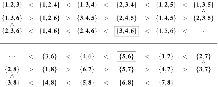
sizel−1 from thecolexicographical orderof each of these sets (separately), defined below.

Definition 13 (Colexicographical Order) Thecolexicographical orderover two sets A and B, where |A|=|B|, is defined by A<B if and only if∃i:(A[i]<B[i]and∀j>i:A[j] =B[j]), where A[i] denotes the i:th element of the set A, when the elements of the set are arranged in numerical order. For example, comparing the setsA={2,3,6}andB={1,4,6}(note that they are already written in numerical order), we obtainA<BbecauseA[2] =3 which is less thanB[2] =4, whileA[3] = B[3] =6. (See Figure 10 for a further illustration.)

Furthermore, the theory also allows for easily computing the smallestp(and hence largestn−p)

for which a valid antichain is obtained: Any choice forpcan be written in a uniquel-cascade form

p =

l

∑

j=1

aj j

, (13)

where the integersa1, . . . ,alcan be computed using a simple greedy approach (for details see Jukna

(2011, p. 146-8) and the code package accompanying this paper). Then, as discussed by Jukna, the

numberqof sets of sizel−1 that are not subsets of the firstpsets in the appropriate

colexicograph-ical order is given by

q =

K l−1

−

l

∑

j=1

aj j−1

. (14)

Thus, if one can pick the smallestpsuch thatp+q≥n, then it is possible to construct a flat antichain

of sizenthat maximizes the number of index sets with sizel−1.

Algorithm 4 thus considers all values of pstarting from 1, until Equations 13 and 14 imply that

there is a flat antichain of size at leastn. It then selects thefirst pindex sets in the colexicographical

order of sets of sizel, and thelast n−psets in the colexicographical order of sets of sizel−1. The

Kruskal-Katona Theorem ensures that the chosen(l−1)-sized sets will not be subsets of the chosen

l-sized sets, thereby guaranteeing the antichain property (Jukna, 2011, p. 146-8). See Figure 10 for an example. Thus, Algorithm 4 returns a set of index sets that minimize the average intervention set size, solving (the directed version of) Problem 1 (a). Figure 9 (middle) shows the optimal average

sizes for various values ofnandK.

{1,2,3} < {1,2,4} < {1,3,4} < {2,3,4} < {1,2,5} < {1,3,5}

>

{1,3,6} > {1,2,6} > {3,4,5} > {2,4,5} > {1,4,5} > {2,3,5}

>

{2,3,6} < {1,4,6} < {2,4,6} < {3,4,6} < {1,5,6} < · · ·

· · · < {3,6} < {4,6} < {5,6} < {1,7} < {2,7}

>

{2,8} > {1,8} > {6,7} > {5,7} > {4,7} > {3,7}

>

{3,8} < {4,8} < {5,8} < {6,8} < {7,8}

Figure 10: Selecting the index sets in colexicographical order forn=30 andK=8. Selecting 16

index sets of size 3 (up to{3,4,6}, in bold) and 14 index sets of size 2 (starting from

{5,6}, in bold), gives a total of 30 index sets and achieves the lowest possible average

intervention set size for the givennandK. Note that none of the selected index sets is a

subset of another, thus the sets form an antichain. If we were to select only 15 index set of size 3 (up to{2,4,6}), we could still only select 14 index sets of size 2 (from{5,6}), ending up with only 29 index sets. If we were to select 17 index sets of size 3 (up to {1,5,6}), we could select 13 index sets of size 2 (from{1,7}), and find 30 index sets,

but the average intervention set size would then be 1/8 higher.

Algorithm 4Obtains a set ofKintervention sets satisfying theorderedpair condition for all ordered

pairs amongnvariables that minimizes the average intervention set size.

Flat(n,K)

Determine the maximum index set sizel from Equation 10, if no suchlexists, the ordered pair condition

cannot be satisfied fornvariables withKexperiments.

Forpfrom1ton,

Find coefficientsa1, . . . ,alfor a cascade presentation ofpin Equation 13.

Calculate the numberqof available index sets of sizel−1by Equation 14.

Ifp+q≥nexit the for-loop.

Choose the index setsI1, . . . ,Ipas thefirstsets of sizelin the colexicographical order.

Choose the index setsIp+1, . . . ,Inas thelastsets of sizel−1in the colexicographical order.

Return the intervention setsJ1, . . . ,JKcorresponding to the index setsI1, . . . ,In.

Trivially, the ceiling of the minimum average intervention set size fornvariables inK

Problem 2 reverses the free parameters and asks for the minimum number of experimentsm(n,r)

given a limitron the maximum size of any intervention set. Cai (1984b) shows that

m(n,r) =

2n r

, if 2≤1

2r

2_{<n. (15)}

With inputK=⌈2n/r⌉, Algorithm 3 generates intervention sets of at most sizer(see Appendix B)—

this verifies thatm(n,r)≤ ⌈2n/r⌉. Cai’s result also gives an exact minimum number of experiments when the maximum intervention set size has to be small (see Figure 9 (bottom)). It can also be used

to construct a lower bound on the maximum intervention set size when the number of experimentsK

is given: Ifm(n,r)>Kfor somerandK, then the maximum intervention set size givennvariables

andKexperiments must be at leastr+1. Again, we use this connection to determine the optimality

of some of the outputs of Algorithm 3 in Figure 9 (top).

For cases when rdoes not satisfy the restrictions of Cai’s result, K¨undgen et al. (2001) use a

similar construction to provide the following bounds:13

min{K|n≤

K ⌈Kr/n⌉

} ≤ m(n,r) ≤ min{K|n≤

K ⌊Kr/n⌋

}, if r≤n

2. (16)

Again the upper bound can be easily verified: With the upper boundKas input, Algorithm 3 will

generate intervention sets of at most sizer (see Appendix C). The lower bound is an application

of classic results of Kleitman and Milner (1973) concerning average index set sizes. In many cases

we can get an improved lower bound onm(n,r)using Algorithm 4 (which optimally minimizes the

average number of interventions per experiment, for givennandK): Find the smallestKsuch that

Algorithm 4 returns intervention sets with an average size less thanr. In this case we know that the

minimum number of experiments given a maximum intervention set size ofrmust be at leastK(see

Figure 9 (bottom)).

Finally, note that Ramsay and Roberts (1996) and Ramsay et al. (1998) have considered the problem equivalent to finding a set of experiments where instead of a limited maximum intervention

set size, the intervention sets are constrained to haveexactly some given size. Sometimes more

experiments are needed in order to satisfy this harder constraint.

6. Background Knowledge

by the set of experiments. Finally, any background knowledge that is equivalent to knowledge of the outcome of some experiment can be described in terms of satisfied pair conditions. In this section, we thus consider the selection of experiments when the experiments only need to satisfy the pair condition for a given subset of all variable pairs, but acknowledge that not all background knowledge is representable in terms of satisfied pair conditions.

When the pair condition only needs to be satisfied for a subset of the variable pairs, the search problem is equivalent to that of finding a minimal cut-covering of a given graph. As described

in Section 3, we represent the satisfaction of theunorderedpair condition by a graph H over the

vertices

V

, where an undirected edge between a pair of variables indicates that the unordered pair

condition isnot yet satisfied for that pair (and hence needs to be satisfied by the experiments we

select), while the absence of an edge indicates it is already satisfied for the pair (and does not need to

be satisfied by our experiments). Similarly, we use adirectedgraphFto represent the satisfaction of

theorderedpair condition, in the analogous way. Essentially, the combinatorial problems discussed

in the two previous sections can thus be interpreted as finding a minimal cut-covering for acomplete

directed or undirected graph, while in this section we consider the problem of finding a minimal

cut-covering for anarbitrarydirected or undirected graph.14

First, consider the satisfaction of the unordered pair condition for an arbitrary subset of all vari-able pairs. Unlike the case without background knowledge, discussed in Sections 4.1, the problem of finding the smallest set of experiments to satisfy the unordered pair condition for a subset of all pairs is known to be hard. Cai (1984a) establishes the connection to minimal graph colorings by

showing (in his Theorem 5) that the smallest cardinality c(H) of a cut-covering of an undirected

graph H relates to its chromatic numberχ(H)(the smallest number of colors required to

vertex-color graphH) as

c(H) = ⌈log₂(χ(H))⌉. (17) The result indicates that the main constraint to reducing the number of experiments are cliques of variables for which the unordered pair condition is not satisfied. Equation 17 constitutes a general-ization of the results shown in Section 4.1. Furthermore, it follows from Cai’s Theorem 6 that the problem of finding a minimal set of experiments given background knowledge for arbitrary pairs

is NP-hard, though constructing the appropriate experimentsgivena graph coloring is very simple.

Various approximation algorithms used for graph coloring could be applied, see for example Welsh and Powell (1967), Motwani and Naor (1993), Halld´orsson (1993), Bussieck (1994) and Liberti et al. (2011) for proposals, bounds and simulations. Algorithm 5 calls a graph coloring method (in the code package we use the simple approximation algorithm by Welsh and Powell, 1967) and constructs intervention sets based on the graph coloring. It results in⌈log₂(χ(H) +c)⌉experiments,

where c is the number of colors the coloring algorithm uses in excess of the chromatic number

χ(H). So it achieves Cai’s optimal bound on the minimum number of experiments (Equation 17) if

the coloring method uses the smallest number of colors.

In certain restricted cases the problem is easier. When the underlying model is known to be acyclic and causally sufficient, and the background knowledge derives from passive observational data or suitable previous experiments, the knowledge can be represented in terms of an (interven-tional) Markov equivalence class. These are sets of causally sufficient acyclic causal models that are