Sign Language Recognition using Sub-Units
Helen Cooper [email protected]
Eng-Jon Ong [email protected]
Nicolas Pugeault [email protected]
Richard Bowden [email protected]
Centre for Vision Speech and Signal Processing University of Surrey
Guildford. GU2 9PY UK
Editors:Isabelle Guyon and Vassilis Athitsos
Abstract
This paper discusses sign language recognition using linguistic sub-units. It presents three types of sub-units for consideration; those learnt from appearance data as well as those inferred from both 2D or 3D tracking data. These sub-units are then combined using a sign level classifier; here, two options are presented. The first uses Markov Models to encode the temporal changes between sub-units. The second makes use of Sequential Pattern Boosting to apply discriminative feature selection at the same time as encoding temporal information. This approach is more robust to noise and performs well in signer independent tests, improving results from the 54% achieved by the Markov Chains to 76%.
Keywords: sign language recognition, sequential pattern boosting, depth cameras, sub-units, signer independence, data set
1. Introduction
This paper presents several approaches to sub-unit based Sign Language Recognition (SLR) cul-minating in a real time KinectTMdemonstration system. SLR is a non-trivial task. Sign Lan-guages (SLs) are made up of thousands of different signs; each differing from the other by minor changes in motion, handshape, location or Non-Manual Featuress (NMFs). While Gesture Recogni-tion (GR) soluRecogni-tions often build a classifier per gesture, this approach soon becomes intractable when recognising large lexicons of signs, for even the relatively straightforward task of citation-form, dic-tionary look-up. Speech recognition was faced with the same problem; the emergent solution was to recognise the subcomponents (phonemes), then combine them into words using Hidden Markov Models (HMMs). Sub-unit based SLR uses a similar two stage recognition system, in the first stage, sign linguistic sub-units are identified. In the second stage, these sub-units are combined together to create a sign level classifier.
Linguists also describe SLs in terms of component sub-units; by using these sub-units, not only can larger sign lexicons be handled efficiently, allowing demonstration on databases of nearly 1000 signs, but they are also more robust to the natural variations of signs, which occur on both an inter and an intra signer basis. This makes them suited to real-time signer independent recognition as described later. This paper will focus on 4 main sub-unit categories based onHandShape,Location,
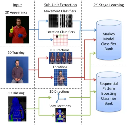
Figure 1: Overview of the 3 types of sub-units extracted and the 2 different sign level classifiers used.
work builds on both the Ha, Tab, Sig, Dez system from the BSL dictionary (British Deaf Associa-tion, 1992) and The Hamburg Notation System (HamNoSys), which has continued to develop over recent years to allow more detailed description of signs from numerous SLs (Hanke and Schmaling, 2004).
three sub-unit types is tested with a Markov model approach to combine sub-units into sign level classifiers. A further experiment is performed to investigate the discriminative learning power of Sequential Pattern (SP) Boosting for signer independent recognition. An overview is shown in Figure 1.
2. Background
The concept of using sub-units for SLR is not novel. Kim and Waldron (1993) were among the first adopters, they worked on a limited vocabulary of 13-16 signs, using data gloves to get accurate input information. Using the work of Stokoe (1960) as a base, and their previous work in telecom-munications (Waldron and Simon, 1989), they noted the need to break signs into their component sub-units for efficiency. They continued this throughout the remainder of their work, where they used phonemic recognition modules for hand shape, orientation, position and movement recogni-tion (Waldron and Kim, 1994). They made note of the dependency of posirecogni-tion, orientarecogni-tion and motion on one another and removed the motion aspect allowing the other sub-units to compensate (on a small vocabulary, a dynamic representation of position is equivalent to motion) (Waldron and Kim, 1995).
The early work of Vogler and Metaxas (1997) borrowed heavily from the studies of sign lan-guage by Liddell and Johnson (1989), splitting signs into motion and pause sections. Their later work (Vogler and Metaxas, 1999), used parallel HMMs on both hand shape and motion sub-units, similar to those proposed by the linguist Stokoe (1960). Kadir et al. (2004) took this further by combining head, hand and torso positions, as well as hand shape, to create a system based on hard coded sub-unit classifiers that could be trained on as little as a single example.
Alternative methods have looked at data driven approaches to defining sub-units. Yin et al. (2009) used an accelerometer glove to gather information about a sign, they then applied discrimi-native feature extraction and ‘similar state tying’ algorithms, to decide sub-unit level segmentation of the data. Whereas Kong and Ranganath (2008) and Han et al. (2009) looked at automatic seg-mentation of sign motion into sub-units, using discontinuities in the trajectory and acceleration to indicate where segments begin and end. These were then clustered into a code book of possible exemplar trajectories using either Dynamic Time Warping (DTW) distance measures Han et al. or Principal Component Analysis (PCA) Kong and Ranganath.
Traditional sign recognition systems use tracking and data driven approaches (Han et al., 2009; Yin et al., 2009). However, there is an increasing body of research that suggests using linguisti-cally derived features can offer superior performance. Cooper and Bowden (2010) learnt linguistic sub-units from hand annotated data which they combined with Markov models to create sign level classifiers, while Pitsikalis et al. (2011) presented a method which incorporated phonetic transcrip-tions into sub-unit based statistical models. They used HamNoSys annotatranscrip-tions combined with the Postures, Detentions, Transitions, Steady Shifts (PDTS) phonetic model to break the signs and an-notations into labelled sub-units. These were used to construct statistical sub-unit models which they combined via HMMs.
2011). At ESIEA they have been using Fast Artificial Neural Networks to train a system which recognises two French signs (Wassner, 2011). This small vocabulary is a proof of concept but it is unlikely to be scalable to larger lexicons. It is for this reason that many sign recognition approaches use variants of HMMs (Starner and Pentland, 1997; Vogler and Metaxas, 1999; Kadir et al., 2004; Cooper and Bowden, 2007). One of the first videos to be uploaded to the web came from Zafrulla et al. (2011) and was an extension of their previous CopyCat game for deaf children (Zafrulla et al., 2010). The original system uses coloured gloves and accelerometers to track the hands. By tracking with a KinectTM, they use solely the upper part of the torso and normalise the skeleton according to arm length (Zafrulla et al., 2011). They have an internal data set containing 6 signs; 2 subject signs, 2 prepositions and 2 object signs. The signs are used in 4 sentences (subject, preposition, object) and they have recorded 20 examples of each. Their data set is currently single signer, making the system signer dependent, while they list under further work that signer independence would be desirable. By using a cross validated system they train HMMs (Via the Georgia Tech Gesture Toolkit Lyons et al., 2007) to recognise the signs. They perform 3 types of tests, those with full grammar constraints achieving 100%, those where the number of signs is known achieving 99.98% and those with no restrictions achieving 98.8%.
2.1 Linguistics
Sign language sub-units can be likened to speech phonemes, but while a spoken language such as English has only 40-50 phonemes (Shoup, 1980), SLs have many more. For example,The Dictio-nary of British Sign Language/English(British Deaf Association, 1992) lists 57 ‘Dez’ (HandShape), 36 ‘Tab’ (Location), 8 ‘Ha’ (Hand-Arrangement), 28 ‘Sig’ (Motion) (plus 4 modifiers, for example, short and repeated) and there are two sets of 6 ‘ori’ (Orientation), one for the fingers and one for the palm.
HamNoSys uses a more combinatorial approach to sub-units. For instance, it lists 12 basic handshapes which can be augmented using finger bending, thumb position and openeness charac-teristics to create a single HandShape sub-unit. These handshapes are then combined with palm and finger orientations to describe the final hand posture. Motion sub-units can be simple linear directions, known as ‘Path Movements’ these can also be modified by curves, wiggles or zigzags.
Motionsub-units can also be modified by locations, for example, move from A to B with a curved motion or move down beside the nose.
In addition, whereas spoken phonemes are broadly sequential, sign sub-units are parallel, with some sequential elements added where required. This means that each of the 57 British Sign Lan-guage (BSL)HandShapeoptions can (theoretically) be in any one of the 36 BSLOrientation combi-nations. In practice, due to the physical constraints of the human body, only a subset of comfortable combinations occur, yet this subset is still considerable.
An advantage of the parallel nature of sub-units, is that they can be recognised independently using different classifiers, then combined at the word level. The reason this is advantageous is that
three methods for extracting sub-units; learnt appearance based (Section 3), hard coded 2D tracking based (Section 4) and hard coded 3D tracking based (Section 5).
3. Learning Appearance Based Sub-units
The work in this section learns a subset of each type of sub-unit using AdaBoost from hand labelled data. As has been previously discussed, not all types of sub-units can be detected using the same type of classifier. ForLocationsub-units, there needs to be correlation between where the motion is happening and where the person is; to this end spatial grid features centred around the face of the signer are employed. ForMotion sub-units, the salient information is what type of motion is occurring, often regardless of its position, orientation or size. This is approached by extracting moment features and using Binary Patterns (BPs) and additive classifiers based on their changes over time. Hand-Arrangementsub-units look at where the hands are in relation to each other, so these are only relevant for bi-manual signs. This is done using the same moment features as for
Motion but this time over a single frame, as there is no temporal context required. All of these sub-unit level classifiers are learnt using AdaBoost (Freund and Schapire, 1995). The features used in this section require segmentation of the hands and knowledge of where the face is. The Viola Jones face detector (Viola and Jones, 2001) is used to locate the face. Skin segmentation could be used to segment the hands, but since sub-unit labels are required this work uses the data set from the work of Kadir et al. (2004) for which there is an in-house set of sub-unit labels for a portion of the data. This data set was created using a gloved signer and as such a colour segmentation algorithm is used in place of skin segmentation.
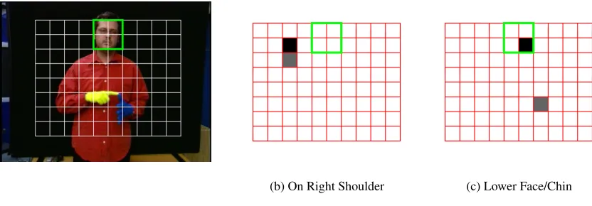
(a) The grid applied over the signer
(b) On Right Shoulder (c) Lower Face/Chin
3.1 LocationFeatures
In order that the sign can be localised in relation to the signer, a grid is applied to the image, dependent upon the position and scale of the face detection. Each cell in the grid is a quarter of the face size and the grid is 10 rectangles wide by 8 deep, as shown in Figure 2a. These values are based on the signing space of the signer. However, in this case, the grid does not extend beyond the top of the signers head since the data set does not contain any signs which use that area. The segmented frame is quantised into this grid and a cell fires if over 50% of its pixels are made up of glove/skin. This is shown in Equation 1 whereRwc is the weak classifier response andΛskin(x,y)is the likelihood that a pixel contains skin. f is the face height and all the grid values are relative to this dimension.
Rwc=
1 if f82 <
x2
∑
i=x1 y2∑
j=y1(Λskin(i,j)>0),
0 otherwise.
Wherex1,y1,x2,y2are given by
∀Gx,∀Gy
x1=Gxf,
x2= (Gx+0.5)f,
y1=Gyf,
y2= (Gy+0.5)f, givenGx={−2.5,−2,−1.5. . .2},
Gy={−4,−3.5,−3. . .0}. (1)
For each of theLocationsub-units, a classifier was built via AdaBoost to combine cells which fire for each particular sub-unit, examples of these classifiers are shown in Figures 2b and (c). Note how the first cell to be picked by the boosting (shown in black) is the one directly related to the area indicated by the sub-unit label. The second cell chosen by boosting either adds to this location information, as in Figure 2b, or comments on the stationary, non-dominant hand, as in Figure 2c.
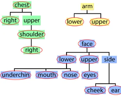
Some of the sub-units types contain values which are not mutually exclusive, this needs to be taken into account when labelling and using sub-unit data. The BSL dictionary (British Deaf Association, 1992) lists severalLocationsub-units which overlap with each other, such as face and mouth or nose. Using boosting to train classifiers requires positive and negative examples. For best results, examples should not be contaminated, that is, the positive set should not contain negatives and the negative set should not contain positives. Trying to distinguish between an area and its sub-areas can prove futile, for example, the mouth is also on the face and therefore there are likely to be false negatives in the training set when training face against mouth. The second stage, sign-level classification does not require the sub-unit classifier responses to be mutually exclusive. As such a hierarchy can be created ofLocationareas and their sub-areas. This hierarchy is shown in Figure 3; a classifier is trained for each node of the tree, using examples which belong to it, or its children, as positive data. Examples which do not belong to it, its parent or its child nodes provide negative data.
hierarchy, for example, face, face lower or face lower mouth which makes finding children and parents easier by using simple string comparisons.
Figure 3: The threeLocationsub-unit trees used for classification. There are three separate trees, based around areas of the body which do not overlap. Areas on the leaves of the tree are sub-areas of their parent nodes. The ringed labels indicate that there are exact examples of that type in the data set.
3.2 MotionandHand-ArrangementMoment Feature Vectors
ForHand-ArrangementandMotion, information regarding the arrangement and motion of the hands is required. Moments offer a way of encoding the shapes in an image; if vectors of moment values per frame are concatenated, then they can encode the change in shape of an image over time.
There are several different types of moments which can be calculated, each of them displaying different properties. Four types were chosen to form a feature vector,m: spatial,mab, central,µab, normalised central, ¯µab and the Hu set of invariant moments (Hu, 1962)
H
1-H
7. The order of a moment is defined asa+b. This work uses all moments, central moments and normalised central moments up to the 3rd order, 10 per type, (00, 01, 10, 11, 20, 02, 12, 21, 30, 03). Finally, the Hu set of invariant moments are considered, there are 7 of these moments and they are created by combining the normalised central moments, see Hu (1962) for full details, they offer invariance to scale, translation, rotation and skew. This gives a 37 dimensional feature vector, with a wide range of different properties.Rwc=
(
1 if
T
wc<Mi,t, 0 otherwise.(2)
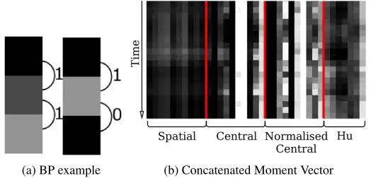
way to the spatial features in Section 3.1, by centring and scaling the image about the face of the signer before computation. For trainingHand-Arrangement, this vector is used to boost a set of thresholds for individual moments, mi on a given frame t, Equation 2. For Motion, temporal information needs to be included. Therefore the video clips are described by a stack of these vectors, M, like a series of 2D arrays, as shown in Figure 4(a) where the horizontal vectors of moments are concatenated vertically, the lighter the colour, the higher the value of the moment on that frame.
(a) BP example (b) Concatenated Moment Vector
Figure 4: Moment vectors and Binary Patterns for two stage classification. (b) A pictorial descrip-tion of moment vectors (normalised along each moment type for a selecdescrip-tion of examples), the lighter the colour the larger the moment value. (a) BP, working from top to bottom an increase in gradient is depicted by a 1 and a decrease or no change by a 0.
3.3 MotionBinary Patterns and Additive Classifiers
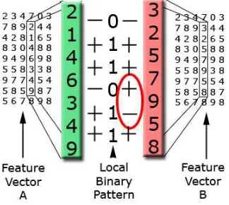
As has been previously discussed, the Motionclassifiers are looking for changes in the moments over time. By concatenating feature vectors temporally as shown in Figure 4(b), these spatio-temporal changes can be found. Component values can either increase, decrease or remain the same, from one frame to the next. If an increase is described as a 1 and a decrease or no change is described as a 0 then a BP can be used to encode a series of increases/decreases. A temporal vec-tor is said to match the given BP if every ‘1’ accompanies an increase between concurrent frames and every ‘0’ a decrease/‘no change’. This is shown in Equation 3 whereMi,t is the value of the component,Mi, at timetandbpt is the value of the BP at framet.
Rwc=||max
∀t (BP(Mi,t))| −1|,
BP(Mi,t) =bpt−d(Mi,t,Mi,t+1),
d(Mi,t,Mi,t+1) =
(
0 ifMi,t ≤Mi,t+1,
1 otherwise. (3)
See Figure 5 for an example where feature vector A makes the weak classifier fire, whereas feature vector B fails, due to the ringed gradients being incompatible.
magnitude of a component over time. The weak classifiers are created by applying a threshold,
T
wc, to the summation of a given component, over several frames. This threshold is optimised across the training data during the boosting phase. For an additive classifier of sizeT, over componentmi, the response of the classifier,Rwc, can be described as in Equation 4.Rwc=
1 if
T
wc≤ T∑
t=0Mi,t,
0 otherwise.
(4)
Boosting is given all possible combinations of BPs, acting on each of the possible components. The BPs are limited in size, being between 2 and 5 changes (3 - 6 frames) long. The additive features are also applied to all the possible components, but the lengths permitted are between 1 and 26 frames, the longest mean length ofMotion sub-units. Both sets of weak classifiers can be temporally offset from the beginning of an example, by any distance up to the maximum distance of 26 frames.
Figure 5: An example of a BP being used to classify two examples. A comparison is made between the elements of the weak classifiers BP and the temporal vector of the component being assessed. If every ‘1’ in the BP aligns with an increase in the component and every ‘0’ aligns with a decrease or ‘no change’ then the component vector is said to match (e.g., case A). However if there are inconsistencies as ringed in case B then the weak classifier will not fire.
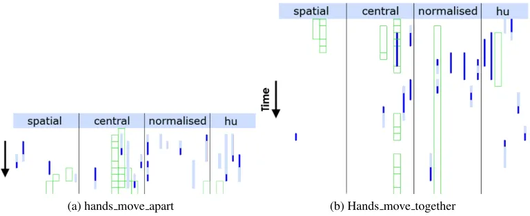
Examples of the classifiers learnt are shown in Figure 6, additive classifiers are shown by boxes, increasing BPs are shown by pale lines and decreasing ones by dark lines. When looking at a sub-unit such as ‘hands move apart’ (Figure 6a), the majority of the BP classifiers show increasing moments, which is what would be expected, as the eccentricity of the moments is likely to increase as the hands move apart. Conversely, for ‘hands move together’ (Figure 6b), most of the BPs are decreasing.
(a) hands move apart (b) Hands move together
Figure 6: Boosted temporal moments BP and additiveMotionclassifiers. The moment vectors are stacked one frame ahead of another. The boxes show where an additive classifier has been chosen, a dark line shows a decreasing moment value and a pale line an increasing value.
long, increasing in steps of 2 and finishing at 26 frames long. Training classification results are then found for each sub-unit and the best length chosen to create a final set of classifiers, of various lengths suited to the sub-units being classified.
4. 2D Tracking Based Sub-Units
Unfortunately, since the learnt, appearance based, sub-units require expertly annotated data they are limited to data sets with this annotation. An alternative to appearance based features is given by tracking. While tracking errors can propagate to create sub-unit errors, the hand trajectories offer significant information which can aid recognition. With the advances of tracking systems and the real-time solution introduced by the KinectTM, tracking is fast becoming an option for real-time, robust recognition of sign language. This section works with hand and head trajectories, extracted from videos by the work outlined by Roussos et al. (2010). The tracking information is used to extractMotion andLocationinformation. HandShapeinformation is extracted via Histograms of Gradients (HOGs) on hand image patches and learnt from labels using random forests. The labels are taken from the linguistic representations of Sign Gesture Mark-up Language (SiGML) (Elliott et al., 2001) or HamNoSys (Hanke and Schmaling, 2004).1
4.1 MotionFeatures
In order to link the x,y co-ordinates obtained from the tracking to the abstract concepts used by sign linguists, rules are employed to extract HamNoSys based information from the trajectories. The approximate size of the head is used as a heuristic to discard ambient motion (that less than 0.25 the head size) and the type of motion occurring is derived directly from deterministic rules on the
(a) Single handed (b) Bimanual: Synchronous (c) Bimanual: Together/Apart
Figure 7: Motions detected from tracking
x and y co-ordinates of the hand position. The types of motions encoded are shown in Figure 7, the single handed motions are available for both hands and the dual handed motions are orientation independent so as to match linguistic concepts.
4.2 LocationFeatures
Similarly the x and y co-ordinates of the sign location need to be described relative to the signer rather than in absolute pixel positions. This is achieved via quantisation of the values into a code-book based on the signer’s head position and scale in the image. For any given hand position(xh,yh) the quantised version(x′h,y′h)is achieved using the quantisation rules shown in Equation 5, where (xf,yf)is the face position and(wf,hf)is the face size.
x′= (xh−xf)/wf,
y′= (yh−yf)/hf. (5)
Due to the limited size of a natural signing space, this gives values in the range ofy′∈ {0..10}and
x′∈ {0..8}which can be expressed as a binary feature vector of size 36, where the x and y positions of the hands are quantised independently.
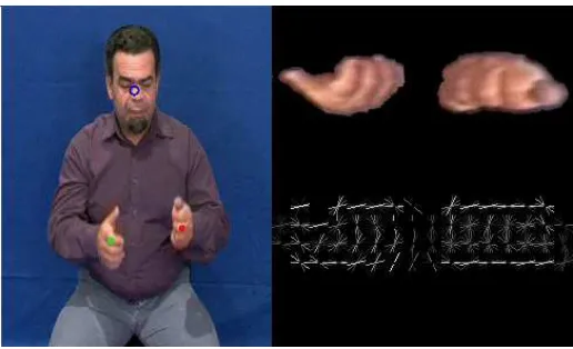
4.3 HandShapeFeatures
Figure 8: Example HOGs extracted from a frame
4.4 HandShapeClassifiers
This work focusses on just the 12 basic handshapes, building multi-modal classifiers to account for the different orientations. A list of these handshapes is shown in Figure 9.
ceeall cee12 cee12open finger2 finger23 finger2345
(153) (200) (107) (4077) (686) (2708)
finger23- fist flat pinch12 pinch12open pinchall
spread (749) (2445) (4612) (571) (845) (830)
Figure 9: The base handshapes (Number of occurrences in the data set)
Unfortunately, linguists annotating sign do so only at thesignlevel while most sub-units occur for onlypart of a sign. Also, not only do handshapes change throughout the sign, they are made more difficult to recognise due to motion blur. Using the motion of the hands, the sign can be split into its component parts (as in Pitsikalis et al., 2011), that are then aligned with the sign annotations. These annotations are in HamNoSys and have been prepared by trained experts, they include the sign breakdown but not the temporal alignment. The frames most likely to contain a static handshape (i.e., those with limited or no motion) are extracted for training.
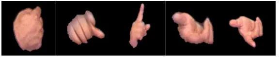
Figure 10: A variety of examples for the HamNoSys/SiGML class ‘finger2’.
The extracted hand shapes are classified using a multi-class random forest. Random forests were proposed by Amit and Geman (1997) and Breiman (2001). They have been shown to yield good performance on a variety of classification and regression problems, and can be trained efficiently in a parallel manner, allowing training on large feature vectors and data sets. In this system, the forest is trained from automatically extracted samples of all 12 handshapes in the data set, shown in Figure 9. Since signs may have multiple handshapes or several instances of the same handshape, the total occurrences are greater than the number of signs, however they are not equally distributed between the handshape classes. The large disparities in the number of examples between classes (see Figure 9) may bias the learning, therefore the training set is rebalanced before learning by selecting 1,000 random samples for each class, forming a new balanced data set. The forest used consists ofN=100 multi-class decision trees Ti, each of which is trained on a random subset of the training data. Each tree node splits the feature space in two by applying a threshold on one dimension of the feature vector. This dimension (chosen from a random subset) and the threshold value are chosen to yield the largest reduction in entropy in the class distribution. This recursive partitioning of the data set continues until a node contains a subset of examples that belong to one single class, or if the tree reaches a maximal depth (set to 10). Each leaf is then labelled according to the mode of the contained samples. As a result, the forest yields a probability distribution over all classes, where the likelihood for each class is the proportion of trees that voted for this class. Formally, the confidence that feature vectorxdescribes the handshapecis given by:
p[c] = 1
Ni
∑
<Nδc(Ti(x)),whereNis the number of trees in the forest,Ti(x)is the leaf of theith treeTiinto whichxfalls, and δc(a)is the Kronecker delta function (δc(a) =1 iff. c=a,δc(a) =0 otherwise).
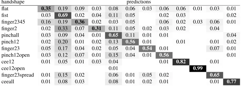
handshape predictions
flat 0.35 0.19 0.09 0.03 0.08 0.06 0.03 0.06 0.06 0.01 0.03 0.01
fist 0.03 0.69 0.02 0.04 0.11 0.05 0.02 0.03 0.02
finger2345 0.16 0.19 0.36 0.02 0.03 0.05 0.06 0.02 0.03 0.06 0.01 finger2 0.02 0.33 0.07 0.31 0.11 0.05 0.02 0.03 0.02 0.04 pinchall 0.03 0.09 0.04 0.01 0.65 0.11 0.01 0.01 0.04 pinch12 0.02 0.20 0.01 0.02 0.13 0.56 0.01 0.01 0.01 0.02 finger23 0.05 0.17 0.04 0.02 0.05 0.04 0.54 0.01 0.07 0.01 pinch12open 0.03 0.12 0.07 0.01 0.15 0.04 0.01 0.56 0.01
cee12 0.01 0.05 0.01 0.03 0.04 0.01 0.82 0.01
cee12open 0.01 0.99
finger23spread 0.01 0.15 0.02 0.06 0.01 0.05 0.02 0.65
ceeall 0.01 0.08 0.03 0.08 0.01 0.02 0.01 0.01 0.77
Table 1: Confusion matrix of the handshape recognition, for all 12 classes.
every non-motion frame, the vector contains a true value in the highest scoring class. The second method applies a fixed threshold (τ=0.25) on the confidences provided by the classifier for each of the 12 handshapes classes. Handshapes that have a confidence above threshold (p[c]>τ) are set to one, and the others to zero. This soft approach carries the double advantage that a) the feature vector may encode the ambiguity between handshapes, which may itself carry information, and b) may contain only zeros if confidences in all classes are small.
5. 3D Tracking Based Sub-Units
With the availability of the KinectTM, real-time tracking in 3D is now a realistic option. Due to this, this final sub-unit section expands on the previous tracking sub-units to work in 3D. The tracking is obtained using the OpenNI framework (Ope, 2010) with the PrimeSense tracker (Pri, 2010). Two types of features are extracted, those encoding theMotionandLocationof the sign being performed.
5.1 MotionFeatures
Again, the focus is on linear motion directions, as with the sub-units described in Section 4.1, but this time with the z axis included. Specifically, individual hand motions in the x plane (left and right), the y plane (up and down) and the z plane (towards and away from the signer). This is augmented by the bi-manual classifiers for ‘hands move together’, ‘hands move apart’ and ‘hands move in sync’, again, these are all now assessed in 3D. The approximate size of the head is used as a heuristic to discard ambient motion (that less than 0.25 the head size) and the type of motion occurring is derived directly from deterministic rules on the x,y,z co-ordinates of the hand position. The resulting feature vector is a binary representation of the found linguistic values. The list of 17 motion features extracted is shown in Table 2.
5.2 LocationFeatures
Locations Motions
Right or Left Hand Bi-manual head left ∆x>λ in sync neck right ∆x<−λ |δ(L,R)|<λ
torso up ∆y>λ and
L shoulder down ∆y<−λ FR=FL
L elbow towards ∆z>λ together
L hand away ∆z<−λ ∆(δ(L,R))<−λ L hip
none ∆L<λ apart
R shoulder ∆R<λ ∆(δ(L,R))>λ R hip
Table 2: Table listing the locations and hand motions included in the feature vectors. The conditions for motion are shown with the label. Wherex,y,zis the position of the hand, either left (L) or right (R),∆indicates a change from one frame to the next andδ(L,R)is the Euclidean distance between the left and right hands. λ is the threshold value to reduce noise and increase generalisation, this is set to be a quarter the head height. FR and FL are the motion feature vectors relating to the right and left hand respectively.
in Figure 11. While displayed in 2D, the regions surrounding the joints are actually 3D spheres. When the dominant hand (in this image shown by the smaller red dot) moves into the region around a joint then that feature will fire. In the example shown, it would be difficult for two features to fire at once. When in motion, the left hand and elbow regions may overlap with other body regions meaning that more than one feature fires at a time.
Figure 11: Body joints used to extract sign locations
6. Sign Level classification
per frame, where fi∈ {0,1}andDis the number of dimensions in the feature vector. This feature vector is then used as the input to a sign level classifier for recognition. By using a binary approach, better generalisation is obtained. This requires far less training data than approaches which must generalise over both a continuous input space as well as the variability between signs (e.g., HMMs). Two sign level classification methods are investigated. Firstly, Markov models which use the feature vector as a whole and secondly Sequential Patten Boosting which performs discriminative feature selection.
6.1 Markov Models
HMMs are a proven technology for time series analysis and recognition. While they have been employed for sign recognition, they have issues due to the large training requirements. Kadir et al. (2004) overcame these issues by instead using a simpler Markov model when the feature space is discrete. The symbolic nature of linguistic sub-units means that the discrete time series of events can be modelled without a hidden layer. To this end a Markov chain is constructed for each sign in a lexicon. An ergodic model is used and a Look Up Table (LUT) employed to maintain as little of the chain as is required. Code entries not contained within the LUT are assigned a nominal probability. This is done to avoid otherwise correct chains being assigned zero probabilities if noise corrupts the input signal. The result is a sparse state transition matrix,Pω(Ft|Ft−1), for each wordω giving a classification bank of Markov chains. During creation of this transition matrix, secondary transitions can be included, wherePω(Ft|Ft−2). This is similar to adding skip transitions to the left-right hidden layer of a HMM which allows deletion errors in the incoming signal. While it could be argued that the linguistic features constitute discrete emission probabilities; the lack of a doubly stochastic process and the fact that the hidden states are determined directly from the observation sequence, separates this from traditional HMMs which cannot be used due to their high training requirements. During classification, the model bank is applied to incoming data in a similar fashion to HMMs. The objective is to calculate the chain which best describes the incoming data, that is, has the highest probability that it produced the observationF. Feature vectors are found in the LUT using an L1 distance on the binary vectors. The probability of a model matching the observation sequence is calculated as
P(ω|s) =υw l
∏
t=1Pω(Ft|Ft−1),
where l is the length of the word in the test sequence andυω is the prior probability of a chain starting in any one of its states. In this work, without grammar,∀ω,υω=1.
6.2 SP Boosting
integers where∀t∈T,ft =1. Following this, we define a SPTof length|T|as:T= (Ti)|i=1T|, where
Tiis an itemset.
In order to use SPs for classification, we first define a method for detecting SPs in an input sequence of feature vectors. To this end, firstly letTbe a SP we wish to detect. Suppose the given feature vector input sequence of |F|frames is F= (Ft)t=1|F|, where Ft is the binary feature vector defined in Section 6. We firstly convertFinto the SPI= (It)|
F|
t=1, whereIt is the itemset of feature vectorFt. We say that the SPTis present inIif there exists a sequence(βi)i=1|T|, whereβi<βj when
i<jand∀i={1, ...,|T|},Ti⊂Iβi. This relationship is denoted with the⊂Soperator, that is,T⊂SI.
Conversely, if the sequence(βi)|i=1T| does not exist, we denote it asT6⊂SI.
From this, we can then define a SP weak classifier as follows: LetTbe a given SP andIbe an itemset sequence derived from some input binary vector sequenceF. ASP weak classifier,hT(I), can be constructed as follows:
hT(I) =
(
1, ifT⊂SI,
−1, ifT6⊂SI.
A strong classifier can be constructed by linearly combining a number (S) of selected SP weak classifiers in the form of:
H(I) = S
∑
i=1αihTii (I).
The weak classifiershi are selected iteratively based on example weights formed during training. In order to determine the optimal weak classifier at each Boosting iteration, the common approach is to exhaustively consider the entire set of candidate weak classifiers and finally select the best weak classifier (i.e., that with the lowest weighted error). However, finding SP weak classifiers corresponding to optimal SPs this way is not possible due to the immense size of the SP search space. To this end, the method of SP Boosting is employed (Ong and Bowden, 2011). This method poses the learning of discriminative SPs as a tree based search problem. The search is made efficient by employing a set of pruning criteria to find the SPs that provide optimal discrimination between the positive and negative examples. The resulting tree-search method is integrated into a boosting framework; resulting in the SP-Boosting algorithm that combines a set of unique and optimal SPs for a given classification problem. For this work, classifiers are built in a one-vs-one manner and the results aggregated for each sign class.
7. Appearance Based Results
(a) Feature vector (b) SP
Figure 12: Pictorial description of SPs. (a) shows an example feature vector made up of 2D motions of the hands. In this case the first element shows ‘right hand moves up’, the second ‘right hand moves down’ etc. (b) shows a plausible pattern that might be found for the sign ‘bridge’. In this sign the hands move up to meet each other, they move apart and then curve down as if drawing a hump-back bridge.
testing purposes. The second stage classifier is trained on the previously used four training examples plus one other, giving five training examples per sign. The results are acquired from the five unseen examples of each of the 164 signs. This is done for all six possible combinations of training/test data. Results are shown in Table 3 alongside the results from Kadir et al. (2004). The first three columns show the results of combining each type of appearance sub-unit with the second stage sign classifier. Unsurprisingly, none of the individual types contains sufficient information to be able to accurately separate the data. However, when combined, the appearance based classifiers learnt from the data are comparable to the hard coded classifiers used on perfectly tracked data. The performance drops by only 6.6 Percentage Points (pp), from 79.2% to 72.6% whilst giving the advantage of not needing the high quality tracking system.
Figure 13, visually demonstrates the sub-unit level classifiers being used with the second stage classifier. The output from the sub-unit classifiers are shown on the right hand side in a vector format on a frame by frame basis. It shows the repetition of features for the sign ‘Box’. As can be seen there is a pattern in the vector which repeats each time the sign is made. It is this repetition which the second stage classifier is using to detect signs.
8. 2D Tracking Results
Ha n d -A rr a n g eme n t L o ca tio n M o tio n C o m b in ed (Ka d ir et a l., 2 0 0 4 )
Minimum (%) 31.6 30.7 28.2 68.7 76.1 Maximum (%) 35.0 32.2 30.5 74.3 82.4 Std Dev 0.9 0.4 0.6 1.5 2.1 Mean (%) 33.2 31.7 29.4 72.6 79.2
Table 3: Classification performance of the appearance based two-stage detector. Using the appear-ance based sub-unit classifiers. Kadir et al. (2004) results are included for comparison purposes.
Figure 13: Repetition of the appearance based sub-unit classifier vector. The band down the right hand side of the frame shows the sub-unit level classifier firing patterns for the last 288 frames, the vector for the most recent frame is at the bottom. The previous video during the 288 frames shows four repetitions of the sign ‘Box’.
Table 4 shows sign level classification results. It is apparent from these results, that out of the independent vectors, the location information is the strongest. This is due to the strong combination of a detailed location feature vector and the temporal information encoded by the Markov chain.
Motion 25.1%
Location 60.5%
HandShape 3.4%
All: WTA 52.7%
All: Thresh 68.4% All + Skips (P(Ft|Ft−2)) 71.4%
Table 4: Sign level classification results using 2D tracked features and the Markov Models. The first three rows show the results when using the features independently with the Markov chain (The handshapes used are non-mutually exclusive). The next three rows give the results of using all the different feature vectors. Including the improvement gained by allowing the handshapes to be non-mutually exclusive (thresh) versus the WTA option. The final method is the combination of the superior handshapes with the location, motion and the second order skips.
Markov Chains SPs Top 1 Top 4 Top 1 Top 4 recall 71.4% 82.3% 74.1% 89.2%
Table 5: Comparison of recall results on the 2D tracking data using both Markov chains and SPs
returned is 68.4%. By including the 2nd order transitions whilst building the Markov chain there is a 3 pp boost to 71.4%.
This work was developed for use as a sign dictionary, within this context, when queried by a video search, the classification would not return a single response. Instead, like a search engine, it should return a ranked list of possible signs. Ideally the target sign would be close to the top of this list. To this end we show results for 2 possibilities; The percentage of signs which are correctly ranked as the first possible sign (Top 1) and the percentage which are ranked in the top 4 possible signs.
This approach is applied to the best sub-unit features above combined with either the Markov Chains or the SP trees. The results of these tests are shown in Table 5. When using the the same combination of sub-unit features as found to be optimal with the Markov Chains, the SP trees are able to improve on the results by nearly 3 pp, increasing the recognition rate from 71.4% to 74.1%. A further improvement is also found when expanding the search results list, within the top 4 signs the recall rate increases from 82.3% to 89.2%.
9. 3D Tracking Results
Test Markov Models SP-Boosting Top 1 Top 4 Top 1 Top 4
In
d
ep
en
d
en
t
1 56% 80% 72% 91%
2 61% 79% 80% 98%
3 30% 45% 67% 89%
4 55% 86% 77% 95%
5 58% 75% 78% 98%
6 63% 83% 80% 98%
Mean 54% 75% 76% 95%
StdDev 12% 15% 5% 4%
Dependent
79% 92% 92% 99.90%
Mean
Table 6: Results across the 20 sign GSL data set.
9.1 Data Sets
Two data sets were captured for training; The first is a data set of 20 GSL signs, randomly chosen and containing both similar and dissimilar signs. This data includes six people performing each sign an average of seven times. The signs were all captured in the same environment with the KinectTMand the signer in approximately the same place for each subject. The second data set is larger and more complex. It contains 40 Deutsche Geb¨ardensprache - German Sign Language (DGS) signs, chosen to provide a phonetically balanced subset of HamNoSys phonemes. There are 15 participants each performing all the signs 5 times. The data was captured using a mobile system giving varying view points.
9.2 GSL Results
Two variations of tests were performed; firstly the signer dependent version, where one example from each signer was reserved for testing and the remaining examples were used for training. This variation was cross-validated multiple times by selecting different combinations of train and test data. Of more interest for this application however, is signer independent performance. For this reason the second experiment involves reserving data from a subject for testing, then training on the remaining signers. This process is repeated across all signers in the data set. The results of both the Markov models and the Sequential Patten Boosting applied to the basic 3D features are shown in Table 6.
Subject Dependent Subject Independent Top 1 Top 4 Top 1 Top 4 Min 56.7% 90.5% 39.9% 74.9%
Max 64.5% 94.6% 67.9% 92.4%
StdDev 1.9% 1.0% 8.5% 5.2%
Mean 59.8% 91.9% 49.4% 85.1%
Table 7: Subject Independent (SI) and Subject Dependent (SD) test results across 40 signs in the DGS data set.
When the SP-Boosting is used, again the dependant case produces higher results, gaining nearly 100% when considering the top 4 ranked signs. However, due to the discriminative feature selection process employed; the user independent case does not show such marked degradation, dropping just 4.9 pp within the top 4 signs, going from 99.9% to 95%. When considering the top ranked sign the reduction is more significant at 16 pp, from 92% to 76%, but this is still a significant improvement on the more traditional Markov model. It can also be seen that the variability in results across signers is greatly reduced using SP-Boosting, whilst signer 3 is still the signer with the lowest percentage of signs recognised, the standard deviation across all signs has dropped to 5% for the first ranked signs and is again lower for the top 4 ranked signs.
9.3 DGS Results
The DGS data set offers a more challenging task as there is a wider range of signers and environ-ments. Experiments were run in the same format using the same features as for the GSL data set. Table 7 shows the results of both the dependent and independent tests. As can be seen with the increased number of signs the percentage accuracy for the first returned result is lower than that of the GSL tests at 59.8% for dependent and 49.4% for independent. However the recall rates within the top 4 ranked signs (now only 10% of the data set) are still high at 91.9% for the dependent tests and 85.1% for the independent ones. Again the relatively low standard deviation of 5.2% shows that the SP-Boosting is picking the discriminative features which are able to generalise well to unseen signers.
As can be seen in the confusion matrix (see Figure 14), while most signs are well distinguished, there are some signs which routinely get confused with each other. A good example of this is the three signs ‘already’, ‘Athens’ and ‘Greece’ which share very similar hand motion and location but are distinguishable by handshape which is not currently modelled on this data set.
10. Discussion
Figure 14: Aggregated confusion matrix of the first returned result for each subject independent test on the DGS data set.
by trajectories alone, thus encoding information about handshape within the moment based clas-sifiers. While this may aid classification on small data sets it makes it more difficult to de-couple the handshape from the motion and location sub-units. This affects the generalisation ability of the classifiers due to the differences between signers.
Where 2D tracking is available, the results are superior in general to the appearance based results. This is shown in the work by Kadir et al. (2004), who achieve equivalent results on the same data using tracking trajectories when compared to the appearance based ones presented here. Unfortunately, it is not always possible to accurately track video data and this is why it is still valid to examine appearance based approaches. The 2D tracking Locationsub-features presented here are based around a grid, while this is effective in localising the motion it is not as desirable as the HamNoSys derived features used in the improved 3D tracking features. The grid suffers from boundary noise as the hands move between cells. This noise causes problems when the features are used in the second stage of classification. With the 3D features this is less obvious due to them being relative to the signer in 3D and therefore the locations are not arbitrarily used by the signer in the same way as the grid is. For example if a signer puts their hands to their shoulders, this will cause multiple cells of the grid to fire and it may not be the same one each time. When using 3D, if the signer puts their hands to their shoulders then the shoulder feature fires. This move from an arbitrary grid to consciously decided body locations reduces boundary effect around significant areas in the signing space.
Instead the SPs look for the discriminative features between the examples, ignoring any signer specific features which might confuse the Markov Chains.
11. Conclusions
This work has presented three approaches to sub-unit based sign recognition. Tests were conducted using boosting to learn three types of sub-units based on appearance features, which are then com-bined with a second stage classifier to learn word level signs. These appearance based features offer an alternative to costly tracking.
The second approach uses a 2D tracking based set of sub-units combined with some appearance based handshape classifiers. The results show that a combination of these robust, generalising fea-tures from tracking and learnt handshape classifiers overcomes the high ambiguity and variability in the data set to achieve excellent recognition performance: achieving a recognition rate of 73% on a large data set of 984 signs.
The third and final approach translates these tracking based sub-units into 3D, this offers user independent, real-time recognition of isolated signs. Using this data a new learning method is introduced, combining the sub-units with SP-Boosting as a discriminative approach. Results are shown on two data sets with the recognition rate reaching 99.9% on a 20 sign multi-user data set and 85.1% on a more challenging and realistic subject independent, 40 sign test set. This demonstrates that true signer independence is possible when more discriminative learning methods are employed. In order to strengthen comparisons within the SLR field the data sets created within this work have been released for use within the community.
12. Future Work
The learnt sub-units show promise and, as shown by the work of Pitsikalis et al. (2011), there are several avenues which can be explored. However, for all of these directions, more linguistically annotated data is required across multiple signers to allow the classifiers to discriminate between the features which are signer specific and those which are independent. In addition, handshapes are a large part of sign, while the work on the multi-signer depth data set has given good results, handshapes should be included in future work using depth cameras. Finally, the recent creation of a larger, multi-signer data set has set the ground work in place for better quantitative analysis. Using this data in the same manner as the DGS40 data set should allow bench-marking of Kinect sign recognition approaches, both for signer dependent and independent recognition. Appearance only techniques can also be verified using the Kinect data set where appropriate as the RGB images are also available though they are not used in this paper. Though it should be noted that this is an especially challenging data set for appearance techniques due to the many varying backgrounds and subjects.
Acknowledgments
References
Y. Amit and D. Geman. Shape quantization and recognition with randomized trees. Neural Com-putation, 9:1545–1588, 1997.
L. Breiman. Random forests. Machine Learning, pages 5–32, 2001.
British Deaf Association. Dictionary of British Sign Language/English. Faber and Faber, 1992.
P. Buehler, M. Everingham, and A. Zisserman. Learning sign language by watching TV (using weakly aligned subtitles). InProceedings of the IEEE Computer Society Conference on Computer Vision and Pattern Recognition, pages 2961 – 2968, Miami, FL, USA, June 20 – 26 2009.
H. Cooper and R. Bowden. Large lexicon detection of sign language. InProceedings of the IEEE
International Conference on Computer Vision: Workshop Human Computer Interaction, pages
88 – 97, Rio de Janario, Brazil, October 16 – 19 2007. doi: 10.1007/978-3-540-75773-3 10.
H. Cooper and R. Bowden. Sign language recognition using linguistically derived sub-units. In
Proceedings of the Language Resources and Evaluation ConferenceWorkshop on the Represen-tation and Processing of Sign Languages : Corpora and Sign Languages Technologies, Valetta, Malta, May17 – 23 2010.
R. Elliott, J. Glauert, J. Kennaway, and K. Parsons. D5-2: SiGML Definition. ViSiCAST Project
working document, 2001.
H. Ershaed, I. Al-Alali, N. Khasawneh, and M. Fraiwan. An arabic sign language computer interface using the xbox kinect. InAnnual Undergraduate Research Conf. on Applied Computing, May 2011.
Y. Freund and R. E. Schapire. A decision-theoretic generalization of on-line learning and an applica-tion to boosting. InProceedings of the European Conference on Computational Learning Theory, pages 23 – 37, Barcelona, Spain, March 13 – 15 1995. Springer-Verlag. ISBN 3-540-59119-2.
J.W. Han, G. Awad, and A. Sutherland. Modelling and segmenting subunits for sign language recognition based on hand motion analysis. Pattern Recognition Letters, 30(6):623 – 633, April 2009.
T Hanke and C Schmaling. Sign Language Notation System. Institute of German Sign Language and Communication of the Deaf, Hamburg, Germany, January 2004. URL
http://www.sign-lang.uni-hamburg.de/projects/hamnosys.html.
M. K. Hu. Visual pattern recognition by moment invariants. IRE Transactions on Information Theory, IT-8:179–187, February 1962.
T. Kadir, R. Bowden, E.J. Ong, and A Zisserman. Minimal training, large lexicon, unconstrained sign language recognition. In Proceedings of the BMVA British Machine Vision Conference, volume 2, pages 939 – 948, Kingston, UK, September 7 – 9 2004.
W.W. Kong and S. Ranganath. Automatic hand trajectory segmentation and phoneme transcription for sign language. InProceedings of the IEEE International Conference on Automatic Face and
Gesture Recognition, pages 1 – 6, Amsterdam, The Netherlands, September 17 – 19 2008. doi:
10.1109/AFGR.2008.4813462.
S.K. Liddell and R.E Johnson. American sign language: The phonological base. Sign Language Studies, 64:195 – 278, 1989.
K. Lyons, H. Brashear, T. L. Westeyn, J. S. Kim, and T. Starner. Gart: The gesture and activity recognition toolkit. In Proceedings of the International Conference HCI, pages 718–727, July 2007.
E. J. Ong and R. Bowden. Learning sequential patterns for lipreading. InProceedings of the BMVA
British Machine Vision Conference, Dundee, UK, August 29 – September 10 2011.
OpenNI User Guide. OpenNI organization, November 2010. Last viewed 20-04-2011 18:15.
V. Pitsikalis, S. Theodorakis, C. Vogler, and P. Maragos. Advances in phonetics-based sub-unit modeling for transcription alignment and sign language recognition. InProceedings of the Inter-national Conference IEEE Computer Society Conference on Computer Vision and Pattern Recog-nitionWorkshop : Gesture Recognition, Colorado Springs, CO, USA, June 21 – 23 2011.
Prime SensorTMNITE 1.3 Algorithms notes. PrimeSense Inc., 2010. Last viewed 20-04-2011 18:15.
A. Roussos, S. Theodorakis, V. Pitsikalis, and P. Maragos. Hand tracking and affine shape-appearance handshape sub-units in continuous sign language recognition. InProceedings of the
International Conference European Conference on Computer VisionWorkshop : SGA, Heraklion,
Crete, September 5 – 11 2010.
J. E. Shoup. Phonological aspects of speech recognition. In Wayne A. Lea, editor,Trends in Speech Recognition, pages 125 – 138. Prentice-Hall, Englewood Cliffs, NJ, 1980.
T. Starner and A. Pentland. Real-time american sign language recognition from video using hidden markov models. Computational Imaging and Vision, 9:227 – 244, 1997.
W.C Stokoe. Sign language structure: An outline of the visual communication systems of the american deaf. Studies in Linguistics: Occasional Papers, 8:3 – 37, 1960.
P. Viola and M. Jones. Rapid object detection using a boosted cascade of simple features. In Pro-ceedings of the IEEE Computer Society Conference on Computer Vision and Pattern Recognition, volume 1, pages 511 – 518, Kauai, HI, USA, December 2001.
C. Vogler and D Metaxas. Adapting hidden markov models for ASL recognition by using three-dimensional computer vision methods. InProceedings of the IEEE International Conference on Systems, Man, and Cybernetics, volume 1, pages 156 – 161, Orlando, FL, USA, October 12 – 15 1997.
M. B. Waldron and S Kim. Increasing manual sign recognition vocabulary through relabelling. In
Proceedings of the IEEE International Conference on Neural Networks IEEE World Congress on Computational Intelligence, volume 5, pages 2885 – 2889, Orlando, Florida, USA, June 27 – July 2 1994. doi: 10.1109/ICNN.1994.374689.
M. B. Waldron and S Kim. Isolated ASL sign recognition system for deaf persons. IEEE Transac-tions on Rehabilitation Engineering, 3(3):261 – 271, September 1995. doi: 10.1109/86.413199.
M.B. Waldron and D Simon. Parsing method for signed telecommunication. InProceedings of the Annual International Conference of the IEEE Engineering in Engineering in Medicine and
Biology Society: Images of the Twenty-First Century, volume 6, pages 1798 – 1799, Seattle,
Washington, USA, November 1989. doi: 10.1109/IEMBS.1989.96461.
H. Wassner. kinect + reseau de neurone = reconnaissance de gestes. http://tinyurl.com/5wbteug, May 2011.
P. Yin, T. Starner, H. Hamilton, I. Essa, and J.M. Rehg. Learning the basic units in american sign language using discriminative segmental feature selection. In Proceedings of the IEEE
Inter-national Conference on Acoustics, Speech and Signal Processing, pages 4757 – 4760, Taipei,
Taiwan, April 19 – 24 2009. doi: 10.1109/ICASSP.2009.4960694.
Z. Zafrulla, H. Brashear, P. Presti, H. Hamilton, and T. Starner. Copycat - center for accessible technology in sign. http://tinyurl.com/3tksn6s, December 2010. URLhttp://www.youtube.
com/watch?v=qFH5rSzmgFE&feature=related.