Optimal Search on Clustered Structural Constraint for Learning
Bayesian Network Structure
Kaname Kojima [email protected]
Eric Perrier [email protected]
Seiya Imoto [email protected]
Satoru Miyano [email protected]
Human Genome Center, Institute of Medical Science University of Tokyo
4-6-1, Shirokanedai, Minato-ku, Tokyo 108-8639, Japan
Editor: David Maxwell Chickering
Abstract
We study the problem of learning an optimal Bayesian network in a constrained search space; skeletons are compelled to be subgraphs of a given undirected graph called the super-structure. The previously derived constrained optimal search (COS) remains limited even for sparse super-structures. To extend its feasibility, we propose to divide the super-structure into several clusters and perform an optimal search on each of them. Further, to ensure acyclicity, we introduce the concept of ancestral constraints (ACs) and derive an optimal algorithm satisfying a given set of ACs. Finally, we theoretically derive the necessary and sufficient sets of ACs to be considered for finding an optimal constrained graph. Empirical evaluations demonstrate that our algorithm can learn optimal Bayesian networks for some graphs containing several hundreds of vertices, and even for super-structures having a high average degree (up to four), which is a drastic improvement in feasibility over the previous optimal algorithm. Learnt networks are shown to largely outperform state-of-the-art heuristic algorithms both in terms of score and structural hamming distance.
Keywords: Bayesian networks, structure learning, constrained optimal search
1. Introduction
Although structure learning is a fundamental task for building Bayesian networks (BNs), when minimizing a score function, the computational complexity often prevents us from finding optimal BN structures (Perrier et al., 2008). With currently available exact algorithms (Koivisto et al., 2004; Ott et al., 2004; Silander et al., 2006; Singh et al., 2005) and a decomposable score like BDeu, the computational complexity remains exponential, and therefore, such algorithms are intractable for BNs with more than around 30 vertices given our actual computational capacity. For larger systems, heuristic searches like greedy hill-climbing search (HC) or customized versions of this search are employed in practice (Tsamardinos et al., 2006).
can-didate (SC) algorithm. Such algorithms have been empirically shown to outperform unconstrained greedy hill-climbing (Friedman et al., 1999; Tsamardinos et al., 2006). Based on the success of con-strained approaches, Perrier et al. (2008) proposed an algorithm that can learn an optimal BN when an undirected graph is given as a structural constraint. Perrier et al. (2008) defined this undirected graph as a super-structure; the skeleton of every graph considered is compelled to be a subgraph of the super-structure. This algorithm can learn optimal BNs containing up to 50 vertices when the average degree of the super-structure is around two, that is, a sparse structural constraint is assumed. However, its feasibility remains limited.
Independently, Friedman et al. (1999) suggested that when the structural constraint is a directed graph (in the case of SC), an optimal search can be carried out on the cluster tree extracted from the constraint. This cluster-based approach could potentially increase the feasibility of optimal searches; nevertheless, the algorithm proposed in Friedman et al. (1999) requires to be given a directed graph-based constraint and to extract a cluster tree. For the latter, a large cluster might be generated, preventing an optimal search from being carried out.
Another potential approach is to search the best BN by checking the network obtained by with-drawing edges in cycles one-by-one, beginning from an initial network which is build by connecting children and their optimal parents with directed edges without checking acyclicity as in B&B al-gorithm (de Campos et al., 2009). However, children in the best BN are often selected as the best parents without considering acyclicity if the size of a given data set is sufficient. Thus, for the estimation of the best BN of more than hundred vertices and sufficient data samples, the initial net-work may contain hundreds of small cycles, and it is impossible to check these cycles in the search process.
In this study, we take up the concept of a super-structure constraint and propose a cluster-based search algorithm that can learn an optimal BN given the constraint. Therefore, unlike in Friedman et al. (1999), our algorithm uses an undirected graph as the structural constraint. In addition, we use a different cluster decomposition that enables us to consider more complex cases. As Tsamardinos et al. (2006) and Perrier et al. (2008) showed, good approximations of the true super-structure can be obtained by an IT approach like the max-min parent-children (MMPC) method (Tsamardinos et al., 2006).
If the super-structure is divided into clusters of moderate size (around 30 vertices), a constrained optimal search can be applied on each cluster. Then, to find a globally optimal graph, one could con-sider all patterns of directions for the edges between clusters and apply a constrained optimal search on each cluster for every pattern of directions independently and return the best result found. We theorize this idea by introducing ancestral constraints; further, we derive the necessary and sufficient ancestral constrains that we must consider to find an optimal network and introduce a pruning tech-nique to skip superfluous cases. Finally, we develop a super-structure constrained optimal algorithm that extends the size of networks that we can consider by more than one order.
2. Related Works
Given data D for a set of random variables V , learning an optimal BN using a decomposable score like BDeu involves finding a directed acyclic graph (DAG) N∗such that
N∗=arg min
N v∈V
∑
s(v,PaN(v); D), (1)where PaN(v)⊆V is a set of parents for a vertex v in network N and s(v,PaN(v); D)is the value of
the score function for v in N. Hereafter, we omit the subscript N for Pa and D for s. In this section, we introduce some structure learning algorithms to show the motivation of our research.
2.1 Optimal search
Although finding a global optimum, that is, a solution of (1), is NP-hard, several optimal algorithms have been developed (Koivisto et al., 2004; Ott et al., 2004; Silander et al., 2006; Singh et al., 2005). The time complexity has been successfully reduced to O(n2n), where n is the number of vertices in BN (i.e.,|V|=n).
2.2 Hill-climbing
For learning a larger system, heuristic algorithms must be used. Greedy hill-climbing (HC) is one of the most commonly used algorithms in practice. HC only finds local optima, and upgraded versions of this base algorithm have been extensively studied, leading to some improvement in the score and structure of the results (e.g., by using a TABU list).
2.3 Sparse Candidate
To improve HC, Friedman et al. (1999) limited the maximum number of parents and restricted the set of candidate parents for each vertex. They established SC algorithm and introduced the concept of constraining the search space of score-based approaches.
2.4 Max-min Hill-climbing
MMHC is a hybrid method combining an IT approach and a score-based search strategy. Tsamardi-nos et al. (2006) showed that on average, MMHC outperforms other heuristic approaches including SC and HC.
2.5 Constrained Optimal Search
In SC and MMHC, the learnt structures are local optima. Perrier et al. (2008) extended the optimal algorithm of Ott et al. (2004) and established a constrained optimal search (COS) that learns an optimal BN structure whose skeleton is a subgraph of a given undirected graph G= (V,E)called the super-structure, that is, COS aims to find NG∗, the solution of (1), while constraining PaN(v)to
2.6 Optimal Search with Cluster Tree
Friedman et al. (1999) suggested the possibility of optimally searching acyclic subgraphs of a di-graph constructed by connecting each vertex and its pre-selected candidate parents with directed edges without checking acyclicity. Here, unlike MMHC and COS, the structural constraint is rep-resented by a directed graph. An algorithm would proceed by converting the digraph into a cluster tree, where clusters are densely connected subgraphs. Then, it would perform an optimal search on each cluster for every ordering of the vertices contained in the separators of clusters. However, due to the difficulty of building a minimal cluster tree, large clusters can make the search impractical.
2.7 B&B Algorithm
Recently, de Campos et al. (2009) proposed an optimal branch-and-bound algorithm. This algo-rithm constructs an initial directed graph by linking every vertex to its optimal parents although this might create directed cycles. Then, it tries to search every possible case in which the direction of one edge comprising each directed cycle is constrained for keeping acyclicity, and finds optimal parents under the constraints iteratively until DAGs are obtained. After the completion of the full search, the optimal solution is finally given by the best DAG found. In addition, for score functions decomposable into penalization and fitting components, optimal parents under the constraints are further effectively computed using a branch-and-bound technique that was originally proposed by Suzuki et al. (1996). This method is interesting in that it is original and allows the development of an anytime search that returns the best current solution found and an upper bound to the global optimum. When the sample size is small, few directed cycles occur in the initial directed graph and updated graphs because information criteria tend to select a smaller parent set for each vertex in small sample data (Dojer, 2006). However, for a large sample size, due to the occurrence of a large number of directed cycles, the complexity of this method can be practically worse than classic optimal searches.
Thereafter, we will consider the same problem as in the COS approach, that is, to find NG∗, an optimal BN constrained by the super-structure G= (V,E), an undirected graph. In our case, we propose a cluster-based search to reduce the complexity drastically; here, clusters are of a different nature from the ones in Friedman et al. (1999), as shown in the next section.
3. Edge Constrained Optimal Search
In this section, we describe procedures of the proposed algorithm in a bottom-up manner. Under the assumption that the skeleton is separated to small subgraphs, we first describe the definition of ancestral constraints for each subgraph and consider an algorithm to learn an optimal BN on a subgraph under some ancestral constrains. We then explain the procedures in order to efficiently build up an optimal BN on the skeleton by using information of optimal BN on each subgraph under the conditions of ancestral constraints to be considered.
3.1 Ancestrally Constrained Optimal Search for A Cluster
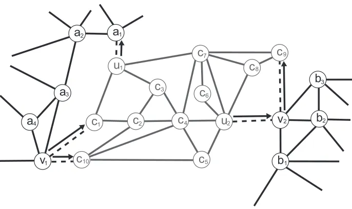
v
a
v
b
b a
a
a
b c
c 1
1 2
3
4 1
1
2 3
7
4 2
5
8 9
2
3
2
1 u
c c
c
c
c c c u
c
6
10
Figure 1: An example of a super-structure to illustrate the definitions we have introduced. The edges of E− are dashed and they define a cluster C (gray). δindicated by arrows is one of the 32 TDMs possible over ECthat defines VCin,δ={v1,v2}and VCout,δ ={u1,u2}.
Definition 1 (cluster and cluster edges) Let C= (VC,EC)be a maximal connected component of
G−. We refer to C as a cluster and call EC⊂E− containing all and only the edges incident to a vertex in VCthe set of cluster edges for C.
Definition 2 (tentative direction map) Given a set of edges EC, we define a tentative direction map (TDM)δon ECas a set of pairs{(e,d),e∈ECand d∈ {←,→}}such that for∀e∈EC, there
uniquely exists d such that(e,d)∈δ. In other words,δassociates a unique direction with each edge in EC.
In the following sections, we show that by successively considering every possibleδon E−and learning the optimal BN on each cluster independently we can reconstruct NG∗. However, to avoid creating cycles over several clusters, our method has to consider all the possible ancestral constraints for a cluster, a notion that we introduce hereafter.
Definition 3 (in-vertex and out-vertex) Considering a cluster C and a TDM δon EC, we define VCin,δ and VCout,δ as VCin,δ={v∈V\VC | ∃va∈VC,({v,va},→)∈δ} and VCout,δ ={v∈VC | ∃va∈V\
VC,({v,va},→)∈δ}, respectively. We drop the subscripts C andδwhen there is no ambiguity. We
call v∈VCin,δan in-vertex and v∈VCout,δ, an out-vertex.
Figure 1 illustrates the previously introduced definitions. In this section, we assume C andδto remain constant.
and
A
(v)be the set of all out-vertices uisuch that(v,ui)∈A
. We say thatA
is a nested ancestralconstraint set (NACS) if and only if for any va and vb in VCin,δ,
A
(va)⊆A
(vb) orA
(va)⊇A
(vb)holds. Finally, given two ACSs
A
andB
, if∀v∈VCin,δ, we have thatA
(v)⊆B
(v), and we say thatB
is stronger than or equal to
A
and denote this relation asA
≤B
.Finally, we recall the definition of a topological ordering and some notions related to it.
Definition 5 (π-linearity and
A
-linearity) Given an orderingπ (i.e., a bijection of [|1,n|]in V ), we say that it is a topological ordering of a BN N if for every v, Pa(v)is included in Pπ(v) ={u∈V |π−1(u)<π−1(v)}, the set of the predecessors of v; in such a case, N is said to beπ-linear. Given an ACS
A
and a BN N, we say that N isA
-linear if and only if it respects all ACs inA
. In addition, in the case of a NACS, there exists a topological orderingπof N such that∀v∈VCin,δand∀u∈A
(v),π−1(u)<π−1(v)holds.
For notational brevity, if π−1(u)<π−1(v) holds for two vertices v and u, we hereafter write u≺πv. Using the previous definitions, we can now prove the validity of our approach.
Theorem 1 There existsδ∗on E−and NACSs
A
∗i for every cluster Ciof G−coherent with a global
optimal BN NG∗. In other words, we can obtain NG∗ by considering the separately obtained optimal BN for every cluster, NACS, and TDM possible.
Proof We consider an optimal DAG NG∗ and one of its topological orderingsπ∗. There exists a unique TDMδ∗ coherent withπ∗. Fromδ∗, we define for every cluster Ci the ACS
A
i∗ such that ∀v∈VCini,δ∗,
A
∗
i(v) =Pπ∗(v)∩VCouti,δ∗.
A
∗
i are definitely NACSs since for every va and vb∈VCini,δ∗
if va ≺π∗ vb, then by definition,
A
i∗(va)⊆A
i∗(vb). Further, the subgraphs Ni∗ of NG∗ on the setsVi=VCi∪V
in
Ci,δ∗ are
A
∗
i-linear (because the definition of
A
i∗is based onπ∗). Furthermore, each Ni∗isan optimal graph on VCi∪V
in
Ci,δ∗given the constraints ofδ
∗and
A
∗i (otherwise, we could build a DAG
having a lower score than NG∗). Therefore, if we independently compute an optimal BN for every cluster, for every TDM and every NACS, and return the best combination, we can build a globally optimal BN on V .
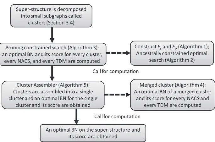
From Theorem 1, the ACS to be considered is limited to only NACS, and NG∗ can be obtained by searching the best combination of an optimal BN separately obtained on every cluster and for every NACS and every TDM. Figure 2 shows the flowchart of the search strategy of our approach. First, an optimal BN and its score on every cluster for every NACS and every TDM are computed. Then, by using this information, an optimal BN and its score on a cluster obtained by merging two clusters are computed for every NACS and every TDM. After the repeated computation of optimal BNs and scores on merged clusters, an optimal BN and its score on a single cluster covering the super-structure are finally obtained. The details and validity of the algorithms shown in the flowchart are discussed in later sections.
Pruning constrained search (Algorithm 3): an opmal BN and its score for every cluster,
every NACS, and every TDM are computed
Merged cluster (Algorithm 4): An opmal BN of a merged cluster
and its score for every NACS and every TDM are computed
Construct Fsand Fp(Algorithm 1);
Ancestrally constrained opmal search (Algorithm 2) Super-structure is decomposed
into small subgraphs called clusters (Secon 3.4)
Cluster Assembler (Algorithm 5): Clusters are assembled into a single cluster and an opmal BN for the single
cluster and its score are obtained
An opmal BN on the super-structure and its score are obtained
Call for computaon
Call for computaon
Figure 2: Flowchart of algorithms for the computation of an optimal BN on a super-structure. The details of these algorithms are discussed in later sections.
Definition 6 (Perrier et al. 2008) For every v∈V and every X⊆
N
(v), we define Fp(v,X)as beingthe best parent set for v included in X and Fs(v,X)as the associated score:
Fs(v,X) = min
Pa⊆Xs(v,Pa),
Fp(v,X) = arg min
Pa⊆Xs(v,Pa).
Further, considering a cluster C,δ, and
A
, for every X ⊆VC, we define ˆsA(X)to be the best scorepossible for a DAG over X∪VCin,δthat satisfies
A
(the scores of the vertices in Vinare not considered), andℓA(X)to be the last element of a topological ordering (restricted to X ) of an optimal DAG over X∪VCin,δthat satisfiesA
(given the constraints). Later, the subscriptA
is omitted.We first introduce an algorithm described in Perrier et al. (2008) that calculates Fsand Fpusing
dynamic programming and then explain how we adapt the calculation of ˆs andℓto satisfy the TDM and the NACS.
Algorithm 1: Calculate Fsand Fp(Perrier et al., 2008) Input: Score function s and super-structure G
Output: Functions Fpand Fs
2. For all v∈V and all X(6=ø)⊆
N
(v)\ {v}, computeu∗ = arg min
u∈XFs(v,X\ {u}),
Fs(v,X) = min{s(v,X),F(v,X\ {u∗})},
Fp(v,X) =
X if s(v,X)≤Fs(v,X\ {u∗})
Fp(v,X\u∗) otherwise
.
Note that the in-vertices are considered differently in our algorithm; they either have no parents or fixed parents, and can only be parents of few vertices in VC depending on
A
. Thus, although theDAGs considered in the following algorithm are optimal on X∪VCin,δ, the score of v∈VCin,δ (that is fixed depending onδ) is not counted in ˆs(X)since it is the same for every DAG irrespective of whether it is optimal or not.
From Theorem 1, the only orderingsπsuch that u≺πv for every v∈VCin,δand u∈
A
(v)are to be considered. Therefore, for w∈VC and v∈VCin,δ, v can be a parent of w if and only if v≺πw,implying u≺πw for every u∈
A
(v). Therefore, we do not need to consider v∈VCin,δin our ordering since we can infer whether v can be a parent of w by checking if it is ordered after all nodes inA
(v). We define for every X ⊆VC the associate set PC(X) =X∪ {v∈VCin,δ|A
(v)⊆X}; in otherwords, for a given topological orderingπover X , the possible parents in X∪VCin,δof w∈X are in PC(Pπ(w))∩
N
(w). Using this result, we can present ACOS:Algorithm 2: AncestrallyConstrainedOptimalSearch
Input: Cluster C, TDMδ, NACS
A
, super-structure G, and functions Fpand Fs(previouslycomputed)
Output: Optimal BN under
A
,δ, G, and its score, ˆs(VC)1. Set ˆs(ø) =∞andℓ(ø) =ø.
2. For all X (6=ø)⊆VC, do:
(a) Computeℓ(X) =arg minv∈X{Fs(v,PC(X\ {v})∩
N
(v)) +sˆ(X\ {v})}.(b) Define ˆs(X)as the minimal score obtained during the previous step.
3. Construct N∗, an optimal
A
-linear BN over VC, using Fpandℓ, and return N∗and its scoreˆ s(VC).
In Algorithm 2, the computation of Fs and Fp is carried out during preprocessing because it does
not depend onδand
A
. Step 3 can be completed in linear time in n and is presented in Perrier et al. (2008). To prove the correctness of ACOS, we explain the computation ofℓin step (a).v
a
v
c
c
1
1
1 1
2 3
7
4 2
5
8 9
2
u
c
c
c
c
c
c
c
u
c
610
Figure 3: If this graph is the best
A
-linear DAG withA
={(v1,u1)}, since both v1and v2are notancestors of u1and u2, its strongest NACS is
B
withB
(v1) =B
(v2) ={u1,u2}. Therefore,this graph is optimal for all seven NACSs included between
A
andB
.parents. Moreover, as stated previously, w∈VCin,δ such that
A
(w)⊆X\ {v} can also be a parent of v while satisfying ACs. Consequently, after adding the structural constraint G, the best score for v is Fs(v,PC(X\ {v})∩N
(v)). Finally, since v cannot be a parent of any nodes in X\ {v}, the best score over this set is ˆs(X\ {v}). Thus, step (a) of Algorithm 2 finds the best sink for X and correctly defines ℓ(X) and ˆs(X). Finally, as explained in Perrier et al. (2008), we can re-build an optimal orderingπ∗over VC by usingℓand obtain an optimal DAG by assigning∀v∈VC,Pa(v) =Fp(v,PC(Pπ∗(v))∩
N
(v)).3.2 Pruning
Following Theorem 1, we know that ACOS has to be computed only for all NACSs. Although the number of NACSs can be shown to be less than O(|EC|!) (because all NACSs can be generated through orderings of Vin
C,δ∪VCout,δ), it is experimentally worse than exponential in the number of
cluster edges. Fortunately, different NACSs frequently lead to the same optimal networks, and many NACS do not need to be considered. For the cluster C and TDM δ shown in Figure 1, Figure 3 shows an optimal BN N under NACS
A
={(v1,u1)}. Since both v1and v2are not ancestorsof u1 and u2, its strongest NACS is
B
={(v1,u1),(v1,u2),(v2,u2),(v2,u2)}. Therefore, N is anoptimal BN of seven NACSs between
A
andB
: {(v1,u1)}, {(v1,u1),(v2,u1)}, {(v1,u1),(v1,u2)}, {(v1,u1),(v1,u2),(v2,u1)}, {(v1,u1),(v1,u2),(v2,u2)}, {(v1,u1),(v2,u1),(v2,u2)}, {(v1,u1),(v1,u2), (v2,u2),(v2,u2)}. The next lemma formally describes this observation.Lemma 1 Let
A
be a NACS andB
, an ACS such thatB
≥A
and that an optimalA
-linear DAG N∗is alsoB
-linear. Then,∀A
′such thatA
≤A
′≤B
, N∗is also an optimalA
′-linear DAG.Proof Since
A
′ is more restrictive thanA
, an optimalA
′-linear DAG N′∗ verifies that s(N′∗)≥By browsing the space of NACS in an order verifying that∀i and j if
A
i≤A
jthen i≤j, and byusing the previous lemma as a pruning criterion, we can considerably reduce the number of NACSs to which ACOS is applied. For a given C andδ, we consider a score-and-network (SN) map SC,δas
a list containing pairs of optimal scores and networks generated by every NACS, not to be pruned. We denote the set of SC,δfor all TDM as SC.
Algorithm 3: PruningConstrainedSearch Input: Cluster C and TDMδ
Output: SN maps SC,δ
1. Initialize an empty set of NACSs U and an empty SN map SC,δ.
2. For every NACS
A
i(ordered such that j≤k ifA
j≤A
k), do:(a) If
A
i∈U , i+ +and restart step (a).(b) Otherwise, learn N∗, an optimal
A
i-linear DAG of score s∗, using Algorithm 2.(c) Let
B
be the ACS containing all ACs satisfied in N∗.(d) ∀
A
′such thatA
i≤
A
′≤B
, addA
′in U .(e) Add the pair(N∗,s∗)to SC,δ.
For enumerating ordered NACSs, see Appendix A. The following theorem shows the correctness of PruningConstrainedSearch.
Theorem 3 For every NACS
A
, there is an optimal DAG in SC,δ.Proof This is trivial since from Lemma 1, we have already found an optimal DAG N∗for the NACS
A
′that are pruned (added to U in step (d)).3.3 Assembling Clusters
Next, we describe how the results of two clusters C1 and C2 are combined. The algorithm given
below builds a set of SN maps SCfor the merged cluster C out of SC1 and SC2 (with VC=VC1∪VC2).
Algorithm 4: MergeCluster
Input: Clusters C1and C2and sets of SN maps SC1 and SC2
Output: Merged cluster C and set of SN maps SC
1. Define C= (VC1∪VC2,EC1∪EC2∪(E
C1∩EC2))
2. For every TDMδof EC, do:
(a) For every pair of TDMδ1andδ2of EC1 and EC2 that satisfy the following conditions: Condition i ∀(e,d)∈δ, then(e,d)∈δi(i=1 or 2),
Condition ii ∀e∈EC1∩EC2,(e,d)∈δ
1if and only if(e,d)∈δ2,
A. Define N∗=N1∗∪N2∗and s∗=s∗1+s∗2
B. If there exists a directed cycle in N∗, restart step i with the next pair. C. Let
A
be the ACS containing all ACs satisfied in N∗.D. If there exists an optimal
A
-linear network in SC,δthat has a score smallerthan s∗, restart step i with the next pair. E. Add the pair(N∗,s∗)to SC,δ.
F. Remove every pair(N′,s′)of SC,δsuch that N′ is
A
-linear and s′>s∗.The next theorem shows that SC,δcontains an optimal BN and its score for every NACS on C.
Theorem 4 If for every pair of TDMsδ1andδ2and for every NACS, SC1,δ1 and SC2,δ2 contain pairs of an optimal BN and its score, then SC,δconstructed by Algorithm 4 contains a pair of an optimal
BN and its score for every NACS.
Proof First, we show that for every NACS
A
over C, we can build an optimalA
-linear BN by merging two optimal networks on C1 and C2 for some NACSsA
1 andA
2. To do so, for a givenTDM δ, let us consider a NACS
A
for C, an optimalA
-linear BN N∗ of score s∗ and one of its topological orderingsπ∗defined over VC(that is also in agreement withδandA
). i is used insteadof 1 and 2. We defineπ∗i the ordering of the vertices in VCi derived fromπ
∗. Further, we call δ i
the TDM of ECi derived from π∗
i; we have that δ1 and δ2 verify trivially conditions (i) and (ii)
stated in step (a) of Algorithm 4. Finally, we define
A
i as a NACS for Ci such that for∀v∈VCini,δi,A
i(v) =Pπi(v)∩VCouti,δi. Given an optimal
A
i-linear network of SCi,δi N∗
i and its score s∗i, let us
con-sider the graph N′=N1∗∪N2∗. This graph is acyclic since it isπ∗-linear by construction. Further, its score s′=s∗1+s∗2 is minimal for
A
-linear; otherwise, one of the Ni∗graphs would not be optimal. Therefore, although N′might be different from N∗, they both have the same score. Therefore, since Algorithm 4 considers every coherent pairδ1 andδ2 (that verify conditions (i) and (ii)) and everypair of NACS, SC,δis correctly constructed.
Given the previous algorithm, we simply need to merge all the clusters to obtain an optimal DAG NG∗ and its score, as explained in the following algorithm.
Algorithm 5: ClusterAssembler Input: Set of all clusters
C
Output: Optimal BN NG∗ and its score s∗
1. ∀C∈
C
, compute SCusing Algorithm 3 for everyδ.2. While|
C
|>1, do:(a) Select a pair of clusters C1and C2such that|(EC1∪EC2)\(EC1∩EC2)|is minimal.
(b) Compute the cluster C and SCby merging C1and C2using Algorithm 4.
(c) Remove C1and C2from
C
, and add C toC
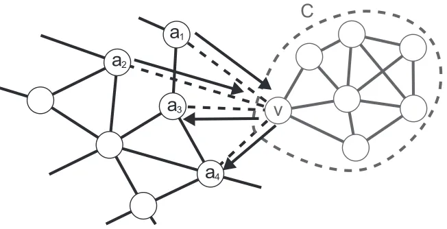
.v
C
a
1a
2a
3a
4Figure 4: An example of super-structure shrinkage. A block C= (VC,EC)(gray) can be separated
from the rest of the super-structure by the removal of a cut-vertex v∈VC. Arrows indicate
the unique TDMδX for X ={a1,a2}.
The correctness of Algorithm 5 is directly derived from Theorem 4. In (a), although we do not prove that the complexity is minimal by merging the clusters that imply less cluster edges for the merged cluster at each step, we decided to use this heuristic. This is because the complexity depends on the number of cluster edges in Algorithm 4; therefore, it is faster to always manipulate a cluster with a small number of cluster edges.
3.4 Preprocessings
In this section, we describe a preprocessing that can drastically reduce the time complexity of our method and the heuristic we used to select the edges in E−.
3.4.1 SUPER-STRUCTURESHRINKAGE
First, we introduce the notions of a block and a block tree of an undirected graph. Their formal definitions are described in Diestel (2005). A block is a biconnected subgraph of the undirected graph, and vertices in the intersection of blocks are called vertices, that is, the removal of cut-vertices separates blocks. A block tree is a tree comprised of blocks as cut-vertices and cut-cut-vertices as edges. We here show leaves of a block tree of the super-structure can be removed if their size is small. Let us consider the case shown in Figure 4 where a block C= (VC,EC)of the super-structure
G can be separated by withdrawing a cut-vertex v∈VCand that C is of a moderate size (|VC|<30).
Then, all edges(v,w), where w6∈VC, are considered as cluster edges; because only v is connected
to cluster edges, no cycle can be created while merging an optimal DAG NC∗ over VC with another
cluster; otherwise, it would imply that there is a cycle in NC∗. Therefore, there is no need of AC and we propose to process this case in a different manner. For every TDMδ, we learn an optimal DAG Nδ∗and its score s∗δ over VC. Then, we replace C by a single vertex ˆv in G to obtain the condensed
super-structure ˆG. For every candidate parent set X of ˆv in ˆG (i.e.,∀X⊆
N
(v)\VC), there exists theFigure 4, unique TDMδX for cluster edges(v,a1),(v,a2),(v,a3), and(v,a4)is indicated by arrows.
Using this observation, we redefine Fson ˆv to be ˆFs(v,Xˆ ) =s∗δX and Fp to be ˆFp(v,Xˆ ) =Nδ∗X; here,
ˆ
Fp is used not only to store the optimal parent set of v in X∪(VC∩
N
(v)) but also to save theoptimal network over C. We can repeat this technique to shrink every small subgraph separated by the removal of a single vertex in G during preprocessing. This can lead to a drastic reduction of complexity in some real cases, as discussed later.
3.4.2 PARTITIONING THESUPER-STRUCTURE INTOCLUSTERS
To apply our algorithm, we need to select a set of edges E−that separates the super-structure into small strongly connected subgraphs (clusters) having balanced numbers of vertices while minimiz-ing the number of cluster edges for each cluster. Such a problem is called graph partitionminimiz-ing. In our case, we employed an algorithm based on edge betweenness centrality that works efficiently for practical networks (Newman et al., 2004).
3.5 Resulting Algorithm
We summarize all results presented thus far in the following algorithm that learns a super-structure constrained optimal network and its score.
Algorithm 6: EdgeConstrainedOptimalSearch (ECOS) Input: Super-structure G= (V,E)and data D
Output: Optimal constrained BN NG∗ and its score s∗
1. ∀v∈V and∀X⊆
N
(v)compute Fs(v,X)and Fp(v,X).2. Shrink every block possible in G to obtain a shrunk super-structure ˆG and the functions ˆFs
and ˆFp.
3. Select E−using the graph partitioning algorithm and obtain the set of all clusters
C
.4. ∀C∈
C
and∀δ; apply Algorithm 3 and obtain the set of SN maps SC.5. Merge all clusters using Algorithm 5 to obtain ˆNG∗ and its score s∗.
6. Expand the subgraphs shrunk during step 2 to obtain NG∗.
Note that after the expansion of shrunk subgraphs, s∗does not change as the scores for these sub-graphs are packed in ˆFs.
3.6 Complexity
In this last section, although it is hardly feasible to derive the complexity of Algorithm 6 in a general case because it strongly depends on the topology of the super-structure used, we propose an upper bound of the complexity depending on a few characteristics of G. Subsequently, we describe some practical generic structures to which ECOS can or cannot be profitably applied. We then present an empirical evaluation of the algorithm over randomly generated networks and real networks, with promising results being found for the latter.
Considering step 1 of ECOS, after defining the maximal degree of G as m=max
v∈V |
N
(v)|, wereason for using a structural constraint because the functions Fp and Fscan be computed in a
lin-ear time for bounded degree structures (m<30). Actually, this is feasible even for large m if an additional constraint on the number of parents c is added, the complexity becoming O(nmc).
Next, if n1 is the size of the largest cluster that has been shrunk (this is a tunable parameter),
and considering that at maximum, the number of cluster edges of a shrunk block m′ is m−1 and the number of TDM is 2m′, given the exponential complexity of calculating ˆs andℓ, we find that the complexity of step 2 is bounded by O(b2m−12n1), where b is the number of blocks shrunk. In other words, if n1is tuned suitably, step 2 has negligible complexity as compared to the subsequent steps.
Similarly, step 3 is negligible since its complexity is only polynomial in n (O(mn3)).
However, step 4 requires a more detailed analysis. Given E−, we define n2=maxC∈C|VC|, the
size of the largest cluster, and k=maxC∈C|EC|, the largest number of cluster edges. The complexity
of ACOS is trivially bounded by O(2n2). Further, because the number of NACS is less than the number of permutations over Vin∪Vout for a given TDM, we have that for every cluster, ACOS is applied at maximum k!2k times. We derive an upper bound complexity for step 4 as O(q2n2k!2k), where q is the number of obtained clusters. Note, however, that the factorial term experimentally appears to be largely overestimated and that ACOS may actually be computed only O(βk)times for
someβ>2.
Finally, at worst, step 5 involves trying every pair of entries in two SN map sets; with the maximum size of cluster edges of merged clusters K, the complexity might theoretically be as bad as O(q(K!2K)2). However, in practice, because a major part of NACS was pruned in step 4, many
pairs are pruned in step 5, and because all superfluous values of the SN maps are eliminated in Algorithm 4, its complexity is closer to O(qβk).
Following those rough upper bounds, we can derive some generic super-structures that are fea-sible for any number of vertices while not being na¨ıve. For example, considering step 2, any super-structure whose block tree contains only small blocks (less than 30 vertices) is feasible. Otherwise, we can consider all the networks that can be generated by the following method:
• Generate an undirected graph G0of low maximal degree (m<10).
• Replace every vertex viby a small graph Ci(up to 20 or slightly more) and randomly connect
all edges connected to viin G0to vertices in Ci.
If ECOS can select all edges between clusters for such networks while defining E−, the search should finish in reasonable time even for larger networks (up to several hundreds of vertices). Con-versely, if a super-structure contains a large clique (containing more than 30 vertices), ECOS cannot finish as other optimal searches. To conclude, our algorithm may be a decisive breakthrough in some real cases where neither optimal searches nor COS can be applied because of a large number of vertices or a high average degree.
4. Experimental Evaluation
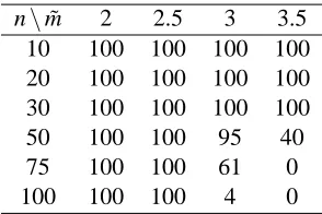
n\m˜ 2 2.5 3 3.5
10 100 100 100 100
20 100 100 100 100
30 100 100 100 100
50 100 100 95 40
75 100 100 61 0
100 100 100 4 0
Table 1: Number of times the computation finished within one day for a random graph of n vertices and average degree ˜m.
Algorithm m˜ 2 2.5 3 3.5
ECOS δm˜ 1.06 1.08 1.15 1.25
nmax(m˜) 355 273 151 93
COS δm˜ 1.50 1.63 1.74 1.81
nmax(m˜) 51 43 38 35
Table 2: Values of coefficientsδm˜ and nmax(m˜) of ECOS and COS for average degree of
super-structure ˜m. δm˜ is the estimated base of exponential time complexity and nmax(m˜)is the
feasible size of the super-structure for computation.
those of MMHC and greedy hill-climbing. All the computations in the following experiments were performed on machines having 3.0 GHz Intel Xeon processors with a Core microarchitecture (only one core was used for each experiment).
4.1 Benefit in Terms of Complexity
In the first series of experiments, we aimed to evaluate the average complexity of ECOS depending on n and ˜m, the average degree of G. Since the feasibility of ECOS depends on the pruning of the search space, the theoretical derivation of the practical time complexity is difficult. Here, we hypothesize that the average complexity is in the form of O(δn
˜
m), and then estimateδm˜. Let tm˜,n be
the time required for a network of n vertices and average degree ˜m. Under our assumption of time complexity, tm˜,nis given by
tm˜,n=const·δnm˜, (2)
where const indicates the dependency of the implementation and machine specifications. From Equation (2), we have that δm˜ =exp(1n(logtm˜,n−log const)). Because log constn can be ignored for
large n, δm˜ can be estimated by exp(logtnm˜,m). For ∀m˜ ∈ {2,2.5,3,3.5} and ∀n∈ {10,20,30,50,75,100}, we generate 100 random networks and we apply ECOS using 1,000 artificially generated samples in each case. We compute the average time ˜tm˜,n that is required and
calculateδm˜,n=exp(log(n˜tm˜,n)). If our hypothesis is correct, δm˜,nshould converge toδm˜ while n
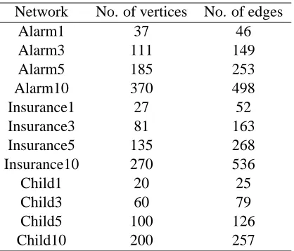
Network No. of vertices No. of edges
Alarm1 37 46
Alarm3 111 149
Alarm5 185 253
Alarm10 370 498
Insurance1 27 52
Insurance3 81 163
Insurance5 135 268
Insurance10 270 536
Child1 20 25
Child3 60 79
Child5 100 126
Child10 200 257
Table 3: Characteristics of the real networks considered in the computational experiment.
than one day. Hence, we probably underestimate δm˜ slightly; nevertheless, here, we attempt to
derive the exponential nature of the average complexity and not the real value of the constants. Fur-ther, the following results are sufficient to obtain a rough estimate. The number of times we finished the calculation for each pair of parameters is listed in Table 1. Due to the small ratio of finished experiments for ˜m=3 and 3.5, we selected the valuesδ3,75,δ3.5,50 forδ3 andδ3.5 , respectively.
Further, for every average degree, we evaluated the maximal number of vertices nmax(m˜)feasible from the value ofδm˜ calculated as proposed in Perrier et al. (2008).
Table 2 lists the values ofδm˜ and nmax(m˜)for ECOS and COS. We should note that nmax(m˜)of
ECOS for ˜m=3 and 3.5 is overestimated since in this case,δm˜ is underestimated because only the
computations that finished were used to calculate it. In practice, nmax(m˜)of ECOS for ˜m=3 and 3.5 are respectively around 75 and 50 from the results listed in Table 1; therefore, we can clearly see the practical advantage of ECOS over COS, and the improvement in terms of feasibility achieved by our method. In addition, we should emphasize that random networks penalize the results of ECOS because they do not have a logical partitioning. In real cases, we can hope that super-structures can be efficiently partitioned, enabling better performances for ECOS.
4.2 Case Study
Model Sample Size α Coverage Average Degree
Alarm5
1000
true 1.00±0.00 2.74±0.00 0.01 0.77±0.00 2.29±0.00 0.02 0.78±0.00 2.40±0.00 0.05 0.80±0.00 2.67±0.00 10000
true 1.00±0.00 2.74±0.00 0.01 0.94±0.00 2.67±0.00 0.02 0.94±0.00 2.77±0.00 0.05 0.95±0.00 3.01±0.00
Alarm10
1000
true 1.00±0.00 2.69±0.00 0.01 0.78±0.00 2.34±0.00 0.02 0.80±0.00 2.49±0.00 0.05 0.81±0.00 2.87±0.00 10000
true 1.00±0.00 2.69±0.00 0.01 0.95±0.00 2.70±0.00 0.02 0.95±0.00 2.84±0.00 0.05 0.96±0.00 3.14±0.00
Insurance5
1000
true 1.00±0.00 3.97±0.00 0.01 0.64±0.00 2.97±0.00 0.02 0.66±0.00 3.15±0.01 0.05 0.68±0.00 3.52±0.01 10000
true 1.00±0.00 3.97±0.00 0.01 0.80±0.00 3.43±0.00 0.02 0.81±0.00 3.53±0.00 0.05 0.83±0.00 3.73±0.01
Insurance10
1000
true 1.00±0.00 3.97±0.00 0.01 0.64±0.00 3.00±0.00 0.02 0.66±0.00 3.22±0.00 0.05 0.67±0.00 3.63±0.01 10000
true 1.00±0.00 3.97±0.00 0.01 0.80±0.00 3.46±0.00 0.02 0.81±0.00 3.57±0.00 0.05 0.82±0.00 3.81±0.01
Child5
1000
true 1.00±0.00 2.52±0.00 0.01 0.84±0.00 2.32±0.00 0.02 0.86±0.00 2.39±0.00 0.05 0.88±0.00 2.50±0.00 10000
true 1.00±0.00 2.52±0.00 0.01 1.00±0.00 2.53±0.00 0.02 1.00±0.00 2.55±0.00 0.05 1.00±0.00 2.57±0.00
Child10
1000
true 1.00±0.00 2.57±0.00 0.01 0.82±0.00 2.3±0.00 0.02 0.84±0.00 2.38±0.00 0.05 0.87±0.00 2.510±0.00 10000
true 1.00±0.00 2.57±0.00 0.01 0.99±0.00 2.58±0.00 0.02 0.99±0.00 2.61±0.00 0.05 0.99±0.00 2.65±0.00
Table 4: Coverage and average degree of super-structures for each experimental condition (mean±
standard deviation).
9 7 9 8 9 9 1 0 0 1 0 1 1 0 2 EC O S MMH C H
C ECO S
MMH C
H
C ECO S
MMH C
H
C ECO S
MMH C
H C
SS(True) SS(α=0.01) SS(α=0.02) SS(α=0.05)
BD
e
u
x104
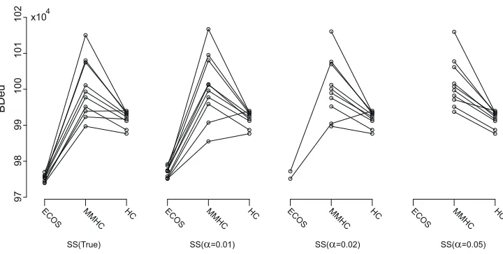
Figure 5: BDeu scores for ten data sets of Alarm10 with 10,000 samples.
0 1 0 0 2 0 0 3 0 0 4 0 0 5 0 0 EC O S MMH C
HC EC O
S MMH
C
HC EC O
S MMH
C
HC EC O
S MMH
C HC
SS(True) SS(α=0.01) SS(α=0.02) SS(α=0.05)
SH
D
Figure 6: Values of SHD for ten data sets of Alarm10 with 10,000 samples.
summarized the ratio of true edges learnt (this ratio is called coverage) and the average degree of the super-structures in Table 4.
For every experimental condition, the algorithms are compared both in terms of score (we used the negative BDeu score, that is, smaller values are better) and structural hamming distance (SHD, Tsamardinos et al. 2006) that counts the number of differences in the completed partially DAG (CPDAG, Chikdering 2002) of the true network and the learnt one.
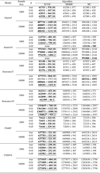
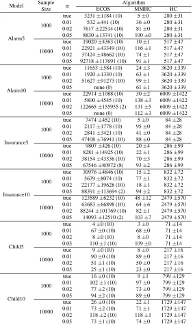
the scaling of the plots for the four conditions are the same, and therefore, the results of HC are the same for the four structural constraints considered. For the true skeleton and super-structures obtained with α=0.01, all ten computations of ECOS finished within two days and ECOS gives the best scores in all the data sets both in terms of BDeu and SHD. In terms of BDeu, HC usually performs better than MMHC, whereas it is the opposite in terms of SHD.
Forα=0.02, only two computations of ECOS finished within two days; nonetheless, the com-puted scores are better than those of MMHC and HC both in terms of BDeu and SHD. For the super-structures ofα=0.05, no computations of ECOS finished within two days. However, every time ECOS finished, it gave better results than both HC and MMHC. With regard to the structural constraint, the best results were obtained when the true skeleton was known. Further, forα=0.01, MMHC is better than HC for two data sets; but for α =0.02, it is better for one data set; and
α=0.05, it is better for no data sets. Because the coverage of super-structures withα=0.01 for Alarm10 with 10,000 samples is already maximal, as shown in Table 4, super-structures for higher
α contain more false-positive edges, which worsens the results of MMHC. We observe the same results in terms of SHD as well.
BDeu and SHD scores for all the experiments are summarized in Tables 5 and 6; for each experimental setup, the best result is in bold and the best result without the knowledge of the true skeleton is underlined. The numbers in parentheses for ECOS represent the number of times ECOS could finish within ten data sets in two days. The cases in which no computation finished are indicated by “none”. Note that all computations of MMHC and HC finished in two days. BDeu and SHD scores of the finished computations are averaged and rounded off to the nearest integer.
While HC outperforms MMHC in BDeu, MMHC outperforms HC in SHD, which agrees with the results in Tsamardinos et al. (2006). A comparison of the results of MMHC and HC suggests that a structural constraint helps to find networks with smaller SHD. However, this should not mislead us into thinking that minimizing a score function is not a good method to learn a graph having a small SHD. In fact, ECOS returns considerably better results than both MMHC and HC in terms of SHD, strongly illustrating the validity of score-based approaches and also the use of a structural constraint.
One could argue that it is possible to increase the quality of the results returned by MMHC by using a largerα. However, as we can see in Table 6, although the score improves with higher α, it is not always the case with the SHD. This is expected because MMHC converges to HC with an increasingα; hence, it is essential in the greedy case to properly selectα. On the other hand, ECOS converges to OS for increasing significance levels. Although in rare cases, SHD slightly worsens with an increasingα, we should generally use as large a significance level as possible when applying ECOS, while ensuring that the algorithm finishes.
Model Sample α Algorithm
Size ECOS MMHC HC
Alarm5
1000
true 61753±376(10) 63294±477 62380±420 0.01 62111±347(10) 63128±428 62380±420 0.02 62015±364(10) 63041±489 62380±420 0.05 61920±387(10) 62959±458 62380±420
10000
true 487734±1109(10) 494611±1986 496108±1104 0.01 488807±1312(10) 495708±2212 496108±1104 0.02 488418±1137(10) 495373±2269 496108±1104 0.05 488182±1132(10) 495359±2638 496108±1104
Alarm10
1000
true 123725±481(10) 126863±857 125156±585 0.01 124406±706(10) 126673±833 125156±585 0.02 124243±750(10) 126456±869 125156±585 0.05 none 126375±831 125156±585 10000
true 975343±943(10) 999973±8022 991888±2144 0.01 976860±1464(10) 1000644±9143 991888±2144 0.02 976150±1404(2) 1000388±8109 991888±2144 0.05 none 1001610±6726 991888±2144
Insurance5
1000
true 81148±341(10) 81551±427 81955±407 0.01 81529±351(10) 81973±458 81955±407 0.02 81449±358(10) 81911±458 81955±407 0.05 81376±338(10) 81862±433 81955±407
10000
true 677374±864(10) 684990±3162 681516±1892 0.01 681584±1707(10) 688579±3521 681516±1892 0.02 680666±1418(10) 687627±2945 681516±1892 0.05 680201±1452(8) 686908±3196 681516±1892
Insurance10 1000
true 162311±453(10) 164039±455 164034±571 0.01 162949±517(10) 164557±711 164034±571 0.02 162890±505(10) 164541±712 164034±571 0.05 162309±46(2) 164541±759 164034±571
10000
true 1354655±768(10) 1371312±3374 1364486±2957 0.01 1361266±1222(10) 1376795±2990 1364486±2957 0.02 1360571±1040(10) 1376111±2542 1364486±2957 0.05 1360627±955(2) 1375645±3224 1364486±2957
Child5
1000
true 71622±324(10) 72057±344 72335±396 0.01 71651±333(10) 72096±368 72335±396 0.02 71648±330(10) 72114±376 72335±396 0.05 71644±329(10) 72059±385 72335±396
10000
true 637783±321(10) 640908±941 644218±2614 0.01 637783±321(10) 640908±941 644218±2614 0.02 637783±321(10) 640908±941 644218±2614 0.05 637783±321(10) 640908±941 644218±2614
Child10
1000
true 142541±250(10) 143847±409 143905±398 0.01 142604±256(10) 143902±415 143905±398 0.02 142590±252(10) 143885±407 143905±398 0.05 142582±255(10) 143896±391 143905±398
10000
true 1271035±684(10) 1277877±2824 1283630±3796 0.01 1271089±690(10) 1278050±2987 1283630±3796 0.02 1271072±683(10) 1277878±2823 1283630±3796 0.05 1271054±685(10) 1277931±2863 1283630±3796
Model Sample α Algorithm
Size ECOS MMHC HC
Alarm5
1000
true 125±10(10) 163±6 215±8 0.01 164±6(10) 177±4 215±8 0.02 164±5(10) 177±4 215±8 0.05 161±5(10) 176±5 215±8
10000
true 21±2(10) 96±15 231±12 0.01 31±2(10) 100±10 231±12 0.02 30±2(10) 101±10 231±12 0.05 30±2(10) 102±9 231±12
Alarm10
1000
true 248±9(10) 321±8 421±15 0.01 317±8(10) 355±13 421±15 0.02 313±9(10) 353±10 421±15 0.05 none 354±11 421±15 10000
true 40±3(10) 215±17 447±22 0.01 54±3(10) 219±16 447±22 0.02 54±4(2) 220±15 447±22 0.05 none 226±12 447±22
Insurance5
1000
true 196±8(10) 205±9 246±8 0.01 207±7(10) 217±5 246±8 0.02 206±7(10) 217±4 246±8 0.05 206±8(10) 217±4 246±8
10000
true 88±1(10) 137±9 184±11 0.01 99±4(10) 146±11 184±11 0.02 99±6(10) 146±9 184±11 0.05 100±6(8) 146±11 184±11
Insurance10 1000
true 378±21(10) 424±11 502±10 0.01 398±21(10) 441±11 502±10 0.02 399±22(10) 441±11 502±10 0.05 376±24(2) 444±9 502±10
10000
true 174±5(10) 280±22 381±23 0.01 198±9(10) 296±21 381±23 0.02 198±12(10) 295±20 381±23 0.05 197±17(2) 295±22 381±23
Child5
1000
true 60±7(10) 70±7 82±8 0.01 71±6(10) 80±5 82±8 0.02 70±6(10) 79±5 82±8 0.05 70±6(10) 78±4 82±8
10000
true 1±0(10) 31±9 43±10 0.01 1±0(10) 31±9 43±10 0.02 1±0(10) 31±9 43±10 0.05 1±0(10) 31±9 43±10
Child10
1000
true 145±9(10) 171±6 182±5 0.01 167±8(10) 188±5 182±5 0.02 165±8(10) 186±6 182±5 0.05 163±8(10) 184±6 182±5
10000
true 8±0(10) 88±16 128±17 0.01 10±3(10) 87±18 128±17 0.02 9±3(10) 87±17 128±17 0.05 8±0(10) 87±18 128±17
Model Sample α Algorithm
Size ECOS MMHC HC
Alarm5
1000
true 3231±1184 (10) 5±0 280±31 0.01 532±441 (10) 36±0 280±31 0.02 7617±22514 (10) 81±0 280±31 0.05 8830±13741 (10) 100±0 280±31 10000
true 19020±4363 (10) 10±1 517±47 0.01 22921±43349 (10) 116±1 517±47 0.02 37424±48662 (10) 74±1 517±47 0.05 92718±117691 (10) 91±1 517±47
Alarm10
1000
true 11653±584 (10) 24±3 3620±339 0.01 1920±1330 (10) 63±1 3620±339 0.02 51627±91273 (10) 99±1 3620±339 0.05 none (0) 61±1 3620±339 10000
true 22914±1088 (10) 30±2 6009±1422 0.01 5800±4545 (10) 138±3 6009±1422 0.02 122665±155955 (2) 131±5 6009±1422 0.05 none (0) 112±3 6009±1422
Insurance5
1000
true 7474±452 (10) 5±0 84±28 0.01 2117±1778 (10) 95±0 84±28 0.02 2841±3421 (10) 41±0 84±28 0.05 47408±76941 (10) 88±0 84±28 10000
true 9807±426 (10) 20±4 286±99 0.01 8281±14925 (10) 22±1 286±99 0.02 38154±43336 (10) 70±3 286±99 0.05 67546±80972 (8) 93±2 286±99
Insurance10 1000
true 30976±4846 (10) 15±2 832±72 0.01 5679±8074 (10) 77±1 832±72 0.02 22177±19628 (10) 18±1 832±72 0.05 88391±113694 (2) 94±2 832±72 10000
true 123589±6232 (10) 48±12 2479±570 0.01 63683±66898 (10) 64±6 2479±570 0.02 85244±101769 (10) 82±1 2479±570 0.05 14093±12510 (2) 103±7 2479±570
Child5
1000
true 4±0 (10) 3±0 71±14 0.01 67±0 (10) 68±0 71±14 0.02 8±0 (10) 8±0 71±14 0.05 110±1 (10) 109±0 71±14 10000
true 9±0 (10) 8±0 217±16 0.01 90±0 (10) 89±0 217±16 0.02 51±1 (10) 50±0 217±16 0.05 25±1 (10) 23±0 217±16
Child10
1000
true 16±0 (10) 9±1 799±129 0.01 102±1 (10) 97±0 799±129 0.02 77±2 (10) 73±0 799±129 0.05 94±2 (10) 89±0 799±129 10000
true 26±0 (10) 22±1 1729±147 0.01 73±2 (10) 71±1 1729±147 0.02 118±2 (10) 118±1 1729±147 0.05 73±1 (10) 74±0 1729±147
5. Discussion and Conclusion
We presented a new BN learning algorithm that finds the optimal network given a structural con-straint, the super-structure. Our algorithm decomposes the super-structure into several clusters and computes optimal networks on each cluster for every ancestral constraint in order to ensure acyclic networks. Experimental evaluations using extended Alarm, Insurance, and Child networks show that our algorithm outperforms state-of-the-art greedy algorithms such as MMHC and HC with a TABU search extension both in terms of the BDeu score and SHD.
It may be possible to develop methods to further increase the feasibility of ECOS; we suggest some ready-to-apply tunings that should make our algorithm faster. First, the algorithm is highly parallelizable since each call to ACOS can be made independently. Further, one could apply a similar shrinkage technique to the interior nodes of the block tree as well if they are of a small size. The algorithm may also benefit from using ECOS recursively instead of ACOS or applying a COS search on the unbreakable clusters rather than a full OS (as is the current case with ACOS). Finally, limiting the maximal size of parent sets by a constant c, as proposed in Section 3.6, improves the feasibility of ECOS because it may also reduce the number of TDMs to consider in some cases. In terms of quality of the learnt network, the best improvements may be realized by developing better algorithms to learn super-structures; in fact, improvements in speed may also be obtained.
If there exist many edges between strongly connected components in the skeleton, the clusters obtained have too many cluster edges; this is usually the main bottleneck of our algorithm that limits its the feasibility. We should emphasize the fact that IT approaches add false-positive edges to the skeleton according to the specified significance level when learning the super-structure. Therefore, although the true skeleton may be well structured (i.e., the true skeleton can be clustered with a small number of cluster edges), the false-positive edges tend to be cluster edges and limit the feasibility of ECOS. For example, the super-structure of Insurance10 obtained withα=0.05 has a smaller average degree than the true skeleton; however, our algorithm did not finish the computation in two days. In addition, since the current version of ECOS depends on a super-structure estimated by the conditional independence test (MMPC), a causal relationship violating faithfulness, for example, XOR parents, can be missed.
Acknowledgments
We would like to thank Andr´e Fujita and Masao Nagasaki for their helpful comments in the initial stage of this work. Computational resources were provided by the Human Genome Center, Institute of Medical Science, University of Tokyo.
Appendix A.
Given a cluster C and a TDM δ (i.e., the corresponding VCin,δ and VCout,δ sets), we define for every possible NACS
A
.Definition 7 (NACS template) The NACS template of
A
is a finite list of pairs of positive integers{(I1,O1),· · ·,(Il,Ol)}such that|VCout,δ| ≥O1>· · ·>Ol≥0 and there are exactly Ik in-vertices vinj
such that|
A
(vinj)|=Ok.For example, let us consider the following NACS
A
with VCin,δ ={v1in, . . . ,vin6} and VCout,δ = {vout, . . . ,vout3 }defined byA
(vin1) ={vout1 ,vout 2 ,vout3 },A
(vin6) ={v1out,vout3 ,vout3 },A
(vin2) ={vout1 ,vout3 },A
(vin4) ={vout3 },A
(vin3) ={vout3 },A
(vin5) =ø.Here, we arranged the AC sets by size to illustrate the fact that due to the definition of NACS, two in-vertices having the same size of ancestral constraint actually have the same ancestral constraint. The NACS template of
A
is{(2,3),(1,2),(2,1),(1,0)}.
Further, following the definition of the NACS template, we have trivially that∑li=1Ii=|VCin,δ|.
Be-cause every NACS admits a unique NACS template, templates define a partition of the space of NACS. Given the template{(I1,O1),· · ·,(Il,Ol)}, there exist
|VCout,δ|
O1
×
O1
O2
× · · · ×
Ol−1
Ol
different ways to assign the out-vertices and
|VCin,δ|
I1
×
|VCin,δ| −I1
I2
× · · · ×
|VCin,δ| −∑l−1i=1Ii
Il
different ways to assign in-vertices. The product of these two values gives the number of NACSs corresponding to this template. All these NACSs can be generated by a brute force method that con-siders every possibility. Next, we introduce an algorithm that generates an ordered list of all NACSs by considering each template successively, starting from(|VCin,δ|,0)and ending with(|VCin,δ|,|VCout,δ|).
Algorithm 7: NACS Enumerator
Input: A set of in-vertices VCin,δand a set of out-vertices VCout,δ
1. Initialize an empty list of NACSs L.
2. Initialize a NACS template NT to(|VCin,δ|,0)and l to 1.
3. While true, do:
(a) Put all the NACSs having NT as template at the end of L.
(b) If NT ={(|VCin,δ|,|VCout,δ|)}, return L.
(c) If l>1 and Ol−1=Ol+1, increment Il−1, otherwise insert(1,Ol+1)in NT
immediately before(Il,Ol)and increment l.
(d) Decrement Il and set Ol to 0.
(e) If Il=0, remove(Il,Ol)from NT and decrement l.
First, we define an order relation for the templates; we say that (Ii,Oi)>(I′j,O′j) if Oi >O′j or
Oi=O′jand Ii>I′j. Then, we say that a NACS template NT is greater than another NT′if(I1,O1)> (I1′,O′1)or(Ij,Oj) = (I′j,O′j)for every j<k and(Ik,Ok)>(Ik′,O′k). We note that if
A
1>A
2, thenthe template of
A
1 is greater than that ofA
2. Therefore, to prove that Algorithm 7 is correct, we simply need to prove that it considers every template in increasing order, that is, that the loop of step 3 generates the successor of a given template NT . Given the constraint that the sum of all Ikis|VCin,δ|,there exist three different cases. If NT is of a size l=1, then NT ={(|VCin,δ|,O1)}and the following
template is{(1,O1+1),(|VCin,δ| −1,0)}, as done in steps (c) and (d). Otherwise, in a similar manner
to the previous case, if Ol−16=Ol+1, the next template will be{(I1,O1),· · ·,(Il−1,Ol−1),(1,Ol+
1),(Il−1,0)}, as in Algorithm 7. Finally, in general, Ol−1=Ol+1 holds, and we simply need to
increment Il−1, decrement Il, and reset Ol to 0. After decrementing Il, it is possible that Il=0, in
which case the last element should be removed. Since Algorithm 7 accesses the direct successor of NT at each step starting from the smaller template(|VCin,δ|,0)until the largest one, we can assert its correctness.
References
C.F. Aliferis, I. Tsamardinos, and A. Statnikov. Causal Explorer: A probabilistic network learn-ing toolkit for discovery. The 2003 International Conference on Mathematics and Engineerlearn-ing Techniques in Medicine and Biological Sciences, 2003.
I.A. Beinlich, H.J. Suermondt, R.M. Chavez, and G.F. Cooper. The ALARM monitoring system: a case study with two probabilistic inference techniques for belief networks. Proceedings of 2nd European Conference on Artificial Intelligence in Medicine, 247–256, 1989.
J. Binder, S. Russell, and P. Smyth. Adaptive probabilistic networks with hidden variables. Machine Learning, 29:213–244, 1997.
D.M. Chickering. Learning equivalence classes of Bayesian-network structures. Journal of Machine Learning Research, 2:445–498, 2002.
C.P. de Campos, Z. Zheng, and Q. Ji. The 26th International Conference on Machine Learning, 2009 (in press).
R. Diestel. Graph Theory 3rd edition. Springer, Berlin, 2005.
N. Dojer. Learning Bayesian networks does not have to be NP-hard. Proceedings of Mathematical Foundations of Computer Science, 305–314, 2006.
N. Friedman, I. Nachman, and D. Pe’er. Learning Bayesian network structure from massive dataset: The “sparse candidate” algorithm. The 15th Conference on Uncertainty in Artificial Intelligence, 196–205, 1999.
M. Koivisto and K. Sood. Exact Bayesian structure discovery in Bayesian networks. Journal of Machine Learning Research, 5:549–573, 2004.
M.E.J. Newman and M. Girvan (2004). Finding and evaluating community structure in networks. Physical Review E, 69(22):26113–26113.
S. Ott, S. Imoto, and S. Miyano. Finding optimal models for small gene networks. Pacific Sympo-sium on Biocomputing, 9:557–567, 2004.
E. Perrier, S. Imoto, and S. Miyano. Finding optimal Bayesian network given a super-structure. Journal of Machine Learning Research, 9:2251–2286, 2008.
T. Silander and P. Myllym¨aki. A simple approach for finding the globally optimal Bayesian network structure. The 22nd Conference on Uncertainty in Artificial Intelligence, 445–452, 2006.
A. Singh and A. Moore. Finding optimal Bayesian networks by dynamic programming (Technical Report). Carnegie Mellon University, 2005.
J. Suzuki. Learning Bayesian belief networks based on the MDL principle: An efficient algorithm using the branch and bound technique. IEICE Transactions on Information and Systems, 356– 367, 1999.
I. Tsamardinos, L.E. Brown, and C.F. Aliferis. The max-min hill-climbing Bayesian network struc-ture learning algorithm. Machine Learning, 65(1):31–78, 2006.