An Error Bound Based on a Worst Likely Assignment
Eric Bax [email protected]
PO Box 60543
Pasadena, CA 91116-6543
Augusto Callejas [email protected]
195 S. Wilson Avenue Apartment 3
Pasadena, CA 91106
Editor: G´abor Lugosi
Abstract
This paper introduces a new PAC transductive error bound for classification. The method uses in-formation from the training examples and inputs of working examples to develop a set of likely assignments to outputs of the working examples. A likely assignment with maximum error deter-mines the bound. The method is very effective for small data sets.
Keywords: error bound, transduction, nearest neighbor, dynamic programming
1. Introduction
An error bound based on VC dimension (Vapnik and Chervonenkis, 1971; Vapnik, 1998) uses uni-form bounds over the largest number of assignments possible from a class of classifiers, based on worst-case arrangements of training and working examples. However, as the number of training examples grows, the probability that training error is a good approximation of working error is so great that the VC error bound succeeds in spite of using uniform bounds based on worst-case as-sumptions about examples. Also, it is easy to compute VC bounds for any number of examples, assuming the VC dimension for the class is known. This makes VC bounds useful and convenient for large data sets, that is, data sets having thousands of examples. However, VC error bounds have some drawbacks: they are ineffective for smaller data sets, and they do not apply to some classifiers, such as nearest neighbor classifiers.
Transductive inference (Vapnik, 1998) is a training method that uses information provided by inputs of working examples in addition to information provided by training examples. The idea is to develop the best classifier for the inputs of the specific working examples at hand rather than develop a classifier that is good for general inputs and then apply it to the working examples. Transductive inference improves on general VC bounds by using the actual working example inputs, instead of a worst-case arrangement of inputs, to find the number of different assignments that classifiers in each training class can produce. The bounds are then used to select among classes, mediating a tradeoff between small classes that are more likely to have good generalization and large classes that are more likely to capture the dynamics of the training data.
training examples. But it also uses information provided by the training procedure rather than just the class of all classifiers that can be produced by the training procedure. However, it requires more computation than VC bounds. In fact, the required computation grows so quickly with data set size that the bound is practical only for small data sets. (Nearest neighbor classifiers are an exception to this limitation; this paper contains an efficient method to compute bounds for them.)
Normally, algorithm designers are concerned about how computation grows as problem size increases, focusing on asymptotic behavior as problem size goes to infinity. This paper does not focus on what happens as data set size goes to infinity—there are already many effective bounds for large data sets. This paper focuses on how much information we can wring out of small data sets. Small data sets do occur in practice, for example in early stage drug tests in medicine and in setting prices and making markets for ad-matching systems that have to deal with tiny markets out in the long tail of information domains. In short, there is “plenty of room at the bottom” for improved error bounds.
The error bound in this paper is based on the fact that if the training and working examples are generated independently and identically distributed (i.i.d.), then each partition of the complete set of training and working examples into a training set and a working set is equally likely. Several error bounds for machine learning are based on this principle. Examples include VC error bounds (Vapnik and Chervonenkis, 1971; Cristianini and Shawe-Taylor, 2000, Section 4.2, p. 55), error bounds for support vector machines (Vapnik, 1998, Chapter 8, pp. 339-343), compression-based error bounds (Littlestone and Warmuth, 1986), and uniform error bounds based on constraints imposed by patterns of agreement and disagreement among classifiers over the working inputs (Bax, 1999). For some other ways of developing and using this idea, refer to Audibert (2004), Blum and Langford (2003), Catoni (2003), Catoni (2004), Derbeko et al. (2003), and El-Yaniv and Gerzon (2005).
This paper is organized as follows. Section 2 introduces concepts and notation for the error bound. Section 3 presents the error bound. Section 4 introduces sampled filters, which reduce com-putation required for the bound. Section 5 analyzes speed and storage requirements for filters based on all partitions and for sampled filters. Section 6 introduces filters based on virtual partitioning, which do not require explicit computation over multiple partitions of the data into different training and working sets. Section 7 gives an efficient algorithm to compute an error bound for a 1-nearest neighbor classifier. Section 8 presents test results comparing bounds produced by different filters on a set of problems. Section 9 is a discussion of possible directions for future research.
2. Concepts and Notation
This paper concerns validation of classifiers learned from examples. Each example Z = (X, Y) includes an input X and a class label Y ∈ {0,1}. We observe
(X1,Y1), ...,(Xt,Yt),Xt+1, ...,Xt+w
that is, inputs and outputs of t training examples and just the inputs of w working examples. (We will use T to denote the set of training examples and W to denote the set of working examples.) A classifier g, which is a mapping from the input space for X to{0,1}, is developed using the observed data. Then classifier g is used to predict the working example outputs Yt+1, . . . , Yt+w associated with Xt+1, . . . , Xt+w.
c= (x1,y1), ...(xt+w,yt+w) (1) from the joint space of inputs and labels, define the error to be
Ec= 1
w
t+w
∑
i=t+1I(g(xi)6=yi),
where I is the indicator function—one if the argument is true and zero otherwise. Let
C=Z1, ...,Zt+w.
Examples in this complete sequence Z1= (X1,Y1), . . . , Zt+w = (Xt+w,Yt+w) are assumed to be drawn i.i.d. from an unknown joint distribution of inputs and labels.
The goal is to produce a PAC (probably approximately correct) bound on EC, the error on complete sequence C.
The bounds in this paper consider different possible assignments to the unknown labels of the working set examples and use permutations of the complete sequence. So we introduce some no-tation around assignments and permuno-tations. For any assignment a∈ {0,1}wand any permutation
σof{1, . . . , t+w}, let C(a, σ) be the sequence that results from assigning labels to the working
examples in C:
∀i∈ {1, ...,w}: Yt+i=ai,
then permuting the sequence according toσ. Let T(a,σ) be the set consisting of the first t examples
in C(a,σ). Let W(a,σ) be the set consisting of the last w examples in C(a,σ). Let g(a,σ) be the
classifier produced by applying the training procedure with T(a,σ) as the training set and W(a,σ)
as the working set. Let E(a,σ) be the error of g(a,σ) over W(a,σ); in other words, let E(a,σ) be the
error E as defined in Equation (1) that would result from using C(a,σ) as the complete sequence. Let a* be the actual (unknown) labels of the working examples. Let Id be the identity permuta-tion. Then
EC=E(a∗,Id).
3. First Error Bound and Algorithm
Section 3.1 presents the error bound. Section 3.2 shows how to compute the bound over partitions instead of permutations. Section 3.3 presents the algorithm for computing the bound.
3.1 Bound
Let Id be the identity permutation. Define a likely set
L={a∈ {0,1}w|P[E(a,σ)≥E(a,Id)]>δ},
max
a∈L E(a,Id). (2)
Theorem 3.1
With probability at least 1−δ,
E(a∗,Id)≤ max
a∈L E(a,Id), (3)
where the probability is over random complete sequences drawn i.i.d. from a joint input-label dis-tribution.
Proof of Theorem 3.1
If a*∈L, then Equation (3) holds. So it suffices to show that
PC(a∗∈/L)≤δ,
where subscript C denotes probability over the distribution of complete sequences C. By the defini-tion of L, the LHS is
=PC[Pσ[E(a∗,σ)≥E(a∗,Id)]≤δ|C],
where subscriptσ denotes probability over the uniform distribution of permutationsσof{1, . . . ,
t+w}. Convert the probability over the distribution of complete sequences to an integral over com-plete sequences:
Z
C
I(Pσ[E(a∗,σ)≥E(a∗,Id)]≤δ|C)p(C)dC,
where p(C) is the pdf of C. Since each permutation of a complete sequence is equally likely, we can replace the integral over complete sequences by an integral over sequences Q of t+w examples followed by an average over permutationsσ0of Q to form complete sets:
= Z
Q 1 (t+w)!
∑
σ0I(Pσ[E(a∗,σ)≥E(a∗,σ0)]≤δ|C=σ0Q)p(Q)dQ. (4)
For each set Q, onlyδ(t+w)! or fewer permutationsσ0can rank in the topδ(t+w)! of all (t+w)! permutations for any statistic, including the statistic E(a*,σ). So,
∀Q :
∑
σ0
I(Pσ[E(a∗,σ)≥E(a∗,σ0)]≤δ|Q)≤δ(t+w)!.
Substitute this inequality into Equation (4), to show it is
≤
Z
Q 1
(t+w)!δ(t+w)!p(Q)dQ.
3.2 From Permutations to Partitions
For each assignment a∈ {0,1}wand each size-t subset S of{1, . . . , t+w}, let T(a, S) be the set (or multi-set) of examples in C(a, Id) indexed by entries of S, and let W(a, S) be the remaining examples in C(a, Id). Refer to the pair T(a, S) and W(a, S) as the partition induced by S. Let g(a, S) be the classifier that results from training with T(a, S) as the training set and W(a, S) as the working set. Let E(a, S) be the error of g(a, S) over W(a, S).
For each permutation σof{1, . . . , t+w}, let σi be the position in C(a, Id) of the example in position i in C(a,σ). Note that
{σ1, ...,σt}=S⇒(T(a,σ),W(a,σ)) = (T(a,S),W(a,S)).
For each S, there is the same number, t!w!, of permutationsσwith{σ1, . . . ,σt}= S, because there are t! ways to order the elements of S inσ1, . . . ,σt and w! ways to order the remaining elements of{1, . . . , t+w} inσt+1, . . . ,σt+w. Since there is this t!w!-to-one mapping from permutations σ
to subsets S with E(a,σ) = E(a, S), the probability over permutations in the definition of L can be
replaced by the following probability over partitions induced by subsets S :
L={a∈ {0,1}w|PS[E(a,S)≥E(a,S∗)]>δ},
where the probability is uniform over size-t subsets S of{1, . . . , t+w}, and S* ={1, . . . , t}. Hence, we can compute errors E(a, S) over size-t subsets S rather than over all permutations in order to compute bound in Equation (2).
3.3 Algorithm
Given an array C of t training examples followed by w working examples and a bound failure prob-ability ceilingδ, Algorithm 3.3.1 returns a valid error bound with probability at least 1−δ. The procedure E(a, S, C), which is not shown, computes E(a, S) by assigning a to the labels of the last
w entries in C, training a classifier using the entries of C indicated by S as the training set and the
remaining entries as the working set, and returning the error of that classifier over that working set.
Algorithm 3.3.1
procedure bound(C, delta)
// Variable bound stores the running max of errors for likely assignments. bound := 0;
// Try all assignments. for (a in {0,1}ˆw)
// Check if error is high enough to be a new max. if (E(a, {1, ..., t}, C) > bound)
// Variable f[i] stores the frequency of E(a, S) = i/w. f[0 ... w] = 0;
// Find error frequencies.
// greater than for S={1, ..., t}. tail := 0;
// Sum the tail.
for (i=E(a, {1, ..., t}, C) to w) tail += f[i]; // If assignment is likely, increase bound. if (tail > delta) bound := E(a, {1, ..., t}, C); end if
end for
return bound; end procedure
4. Sampled Filters and Ranking with Random Tie Breaking
The goal is to reject from L as many false assignments a as possible among those that have E(a,
Id)>E(a*, Id), while only rejecting a* in a fractionδor fewer of cases. The bound process in the previous section rejects assignments a for which E(a, S*) is abnormally high among errors E(a, S) over subsets S of{1, . . . , t+w}, that is, among partitions of the complete sequence into training and working sets. For each assignment a, the process is equivalent to ranking all subsets S in order of
E(a, S), finding the fraction of subsets that outrank S*, even with S* losing all ties, and rejecting a
if the fraction isδor less. Call this filter the complete filter, because it compares S* to all subsets
S. This section introduces alternative filters that do not require computation over all subsets and a
random tie breaking process that ranks S* fairly among subsets S having the same error instead of having S* lose all ties.
4.1 Sampled Filters
The complete filter is expensive to compute. To motivate thinking about alternative filters, note that any filter that accepts a* into L with probability at least 1-δproduces a valid bound. For example, a filter that simply makes a random determination for each assignment, accepting it into L with probability 1-δ, independent of any data about the problem at hand, still produces a valid error
bound. Of course, this random filter is unlikely to produce a strong bound, because it does not preferentially reject assignments a that have high error E(a, S*).
The following sampled filter, based on errors E(a, S) over a random sample of subsets S, re-jects assignments with high error E(a, S*), and it is less expensive to compute than the complete filter. For each assignment a, generate a sample of n size-t subsets S of{1, . . . , t+w}. Generate the sample by drawing subsets i.i.d. with replacement based on a uniform distribution over subsets, or generate the sample by drawing subsets i.i.d. without replacement based on a distribution that is uniform over subsets other than S* and has zero probability for S*. After drawing the sample by either method, add S* to the sample. Then use the sample in place of the set of all subsets S in the algorithm, that is, accept assignment a if the fraction of subsets S in the sample with E(a, S) at least
Theorem 4.1.1
Let R be the set of all size-t subsets of{1, . . . , t+w}. Let M be a set (or multi-set) of entries from R, drawn i.i.d. with replacement based on a uniform distribution over R. Let
LM=
a∈ {0,1}w|P
S∈M∪{S∗}[E(a,S)≥E(a,S∗)]>δ
where the probability is uniform over all sets S in M. Then, with probability at least 1−δ,
E(a∗,S∗)≤ max a∈LM
E(a,S∗), (5)
where the probability is over random complete sequences C drawn i.i.d. from a joint input-label distribution and over random subset samples M.
Proof of Theorem 4.1.1
If a*∈LM, then Equation (5) holds. So we will show
PC,M(a∗∈/LM)≤δ, (6)
where the probability is over the joint distribution of complete sequences C and subset samples M. By the definition of LM, the LHS is
=PC,M[PS∈M∪{S∗}[E(a∗,S)≥E(a∗,S∗)]≤δ|C].
Convert the probability over C into an integral over sequences Q of t+w examples, followed by a probability over permutationsσ0of Q to form complete sets:
Z
Q
Pσ0,M[PS∈M∪{S∗}[E(a∗,S)≥E(a∗,S∗)]≤δ|C=σ0Q]p(Q)dQ, (7)
where the first probability is over a joint distribution ofσ0and M, withσ0drawn uniformly at random from permutations of t+w elements and independently of M. For any fixed sequence Q, consider the expression from within Equation (7):
Pσ0,M[PS∈M∪{S∗}[E(a∗,S)≥E(a∗,S∗)]≤δ|C=σ0Q]. (8)
Define multi-set
H(Q) ={E(a∗,S)|S∈M∪ {S∗}}.
Random draws ofσ0and M make H(Q) a multi-set of random values drawn i.i.d. from a uniform distribution over the set
U(Q) ={E(a∗,S)|S⊆ {1, ...,t+w} ∧ |S|=t}.
Since the elements of H(Q) are drawn i.i.d., the probability that E(a*, S*) ranks in the topδ|H(Q)|of the positions in a ranking of entries in H(Q) is at mostδ. Note that Equation (8) is this probability. So
Substitute this inequality into Equation (7), showing that the LHS of Equation (6) is
≤
Z
Qδ
p(Q)dQ.
Integrate to getδ, completing the proof.
Now consider the case of sampling subsets without replacement:
Theorem 4.1.2
Let R0be the set of all size-t subsets of{1, . . . , t+w}, except for S*. Let M0 be a set of entries from R0, drawn i.i.d. without replacement based on a uniform distribution over R0. Let
LM0 =a∈ {0,1}w|PS∈M0∪{S∗}[E(a,S)≥E(a,S∗)]>δ ,
where the probability is uniform over all sets S in M0. Then, with probability at least 1 − δ,
E(a∗,S∗)≤ max
a∈LM0 E(a,S
∗),
where the probability is over random complete sequences C drawn i.i.d. from a joint input-label distribution and over random subset samples M.
Proof of Theorem 4.1.2
The proof is almost the same as the proof of Theorem 4.1.1, substituting M0 for M. The set
H(Q) becomes a set of random variables drawn i.i.d. from U(Q) without replacement, rather than
with replacement. But with or without replacement, the probability that E(a*, S*) ranks in the topδ
|H(Q)|of the positions in a ranking of entries in H(Q) is at mostδ. Otherwise, the proof is the same.
4.2 Random Tie Breaking
Both the complete filter and the sampled filter accept an assignment if the fraction of a set of subsets
S with E(a, S) at least E(a, S*) is greater thanδ. In essence, if other subsets S have the same error as S*, then this rule errs on the side of safety by treating those subsets S as having greater error than
S*. This ensures that the bound is valid, but it makes the bound weaker than necessary. To close the
gap, use random tie breaking to rank S* at random among the subsets S that have E(a, S) = E(a, S*). Let k be the number of subsets S with the same error as S*, including S* itself. Generate an integer uniformly at random in [1,k] to be the number of subsets S with the same error that rank at or above
S* after random tie breaking. If that number plus the number of subsets S with error greater than for S* is a larger fraction of the partitions thanδ, then accept the assignment.
5. Speed and Storage Requirements for Complete and Sampled Filters
Consider the storage requirements for the bound process. Since the maximum error E(a, S) over assignments in L is obtained by maintaining a running maximum as assignments are added to L, there is no need to store L explicitly. So the storage requirements are mild, including space for a data set, for two classifiers, and for training a classifier.
O(2w
t+w t
)
classifiers. Using the sampled filter instead requires time to train
O(2wn)
classifiers, where n is the number of sample partitions per assignment. Both types of filters can be computed in parallel, using different machines to filter different sets of assignments, each keeping a running maximum of E(a, S*) over accepted assignments, and then finishing by fanning in the maximum over the machines.
To reduce computation, evaluate assignments a for membership in L in decreasing order of E(a,
S*). When the first assignment a is accepted into L, return E(a, S*) as the error bound, and stop.
To order assignments by E(a, S*), train a classifier g, and apply it to each input in W to form the assignment with zero error. Invert that assignment to form the assignment with maximum error. Invert single elements of that assignment to produce assignments with the next greatest error rates. Then invert pairs of elements, then triples, etc. (This technique reduces computation only by a small fraction when the bound is effective; the reduction is only about half for an error bound of 0.5 and even less for smaller error bounds. On the other hand, it does contribute to “fast failure” when the bound is not effective.)
6. Virtual Partitions
Section 6.1 introduces the virtual partition filter. Section 6.2 describes the leave-one-out filter. Section 6.3 presents scoring functions. Section 6.4 suggests a scoring function for support vector machines.
6.1 Virtual Partition Filter
Define a general likely set Lh, based on some function h:
Lh={a∈ {0,1}w|PS[h(a,S)≥h(a,S∗)]>δ},
where the probability is over subsets S of{1, . . . , t+w}. Define a general error bound
Eh(a,S) = max
a∈Lh
E(a,S∗).
If the filter
PS[h(a,S)≥h(a,S∗)]>δ
6.2 Leave-One-Out Filter
For example, let h(a, S) be the number of leave-one-out errors in W(a, S). (A leave-one-out error is an example in C(a) that has a different label than the closest other example in C(a), with distance based on some metric over the input domain.) A filter based on leave-one-out errors excludes assignments a that cause an improbably large fraction of the leave-one-out errors in C(a) to be in the working set. Frequencies of leave-one-out errors in W(a, S) over subsets S can be computed without explicitly iterating over the subsets. The frequencies have a hypergeometric distribution—if there are m leave-one-out errors in C(a), then
PS[h(a,S) = j] =
m j
t+w−m w−j
t+w w
,
where the probability is uniform over size-t subsets S of{1, . . . , t+w}.
Compute the filter for each assignment as follows. Set the labels of Zt+1, . . . , Zt+waccording to
a. Then compute the number of leave-one-out errors in C(a); call it m. Next, compute frequencies:
∀j∈ {max(0,m−t), ...,min(w,m)}: fj=
m j
t+w−m w−j
.
Let j*=h(a,S*), that is, the number of leave-one-out errors in W(a, S*). Let
v=
min(w,m)
∑
j=j∗fj.
For random tie breaking, subtract from v a number drawn uniformly at random from [0, fj∗−1].Then divide by the number of partitions:
t+w w
.
If the result isδor less, then reject assignment a.
6.3 Scoring Functions
In general, let s be a scoring function on examples in C(a) that returns an integer. Let
h(a,S) =
∑
Z∈W(a,S)s(Z).
Let n(Z) be the nearest neighbor to Z in T∪W–{Z}. For example, when counting leave-one-out errors,
s(Z) =
1 i f n(Z).y6=Z.y
0 otherwise
where .y after an example denotes the output, Y, for the example.
s(Z) =|{Q∈T∪W|n(Q) =Z and Q.y6=Z.y}|.
For scoring functions, such as this one, that have a range other than {0,1}, the hypergeometric distribution does not apply. However, dynamic programming allows efficient computation of the frequencies, as follows. Let
ci jk≡
(
A⊆ {1, ...,i} | |A|= j and
∑
b∈A
s(Zb) =k )
,
that is, the number of size-j subsets of the first i examples in C(a) that have sum of scores k. The base cases are
∀(j,k): c0 jk=0
except
c000=1,
and
∀k<0 : ci jk=0.
The recurrence is
ci jk=ci−1,j,k+ci−1,j−1,k−s(i),
where s(i) is the score of example i. The frequencies are:
PS[h(a,S) =k] =ct+w,w,k.
Computing an error bound using virtual partitions requires O(2wpoly(t+w))time because the scor-ing function is computed for each of the 2w assignments. (This assumes O(poly(t+w)) time to compute the filter for each assignment.) The computation requires O(poly(t+w)) space since each assignment can be filtered without reference to others, and the maximum error of a likely assignment can be maintained using a single variable.
6.4 Scoring Functions for SVMs
Now consider filters with virtual partitions for support vector machines (SVMs). A leave-one-out filter can require much computation—for each assignment, training separate SVMs with each example held out in order to compute the number of leave-one-out errors. Joachims discovered a method to bound the number of leave-one-out errors based on the results of training a single SVM on all examples. The method is called εα-estimation (Joachims, 2002, Ch. 5). Computing the
7. Efficient Computation of Error Bounds for 1-Nearest Neighbor Classifiers
When using virtual partitions based on leave-one-out errors to produce an error bound for a 1-nearest neighbor classifier, there is a way to avoid iterating over all assignments to compute the bound. Avoiding this iteration leads to an efficient method to compute an error bound for a 1-nearest neighbor classifier, that is, a method that requires time polynomial in the size of the problem. This section begins with some preliminary concepts before presenting the recurrences and dynamic programming algorithm. Next there is a small example to illustrate the algorithm. Then there are details on how to compute the recurrences efficiently. This section ends with a note on how to extend the algorithm to improve the bounds by allowing random tie breaking for ranking.
7.1 Preliminaries and Concepts
To begin, ensure that each example has a unique nearest neighbor by randomly perturbing the inputs of examples that tie to be nearest neighbors to any example. Perturb by so little that no new nearest neighbor can be introduced. Repeat until each example has a unique minimum distance to another example.
Lemma 7.1.1
This form of random tie breaking makes it impossible for a cycle of three or more examples to have each example in the cycle the nearest neighbor of the next.
The proof is by contradiction. Let n(Z) be the nearest neighbor of example Z in T∪W− {Z}. Suppose there is a cycle of examples Z1, . . . , Zm, Z1 with m >2 and each example the nearest
neighbor of the next, that is,
∀i∈ {1, ...,m}: Zi=n(Zi+1),
and
Zm=n(Z1)
Let d be the distance metric over example inputs. Then
d(Z1,Z2)≤...≤d(Zm,Z1)≤d(Z1,Z2).
For cycles greater than length two, the tie breaking makes equality impossible. So we have
d(Z1,Z2)< ... <d(Zm,Z1)<d(Z1,Z2).
Having the same distance on the left and right implies that the distance from the first example to the second is greater than itself, which is impossible, completing the proof.
Let G be a directed graph with each example in Z1, . . . , Zt+wa node and with edges
{(n(Z1),Z1), ...,(n(Zt+w),Zt+w)},
7.2 Recurrences and Algorithm
Let F(k) be the subtree of F rooted at example Zk, that is, Zk and all nodes that can be reached by following directed sequences of edges from Zk. Let A(i,j,k) be the subset of assignments in{0,1}w that have i leave-one-out errors among the training examples in F(k) and j leave-one-out errors among the working examples of F(k). Let n(Z,T) be the nearest neighbor of example Z among the training examples. Define
ei jky=
max
a∈A(i,j,k) |{Z∈F(k)∩W|Z.y=y and Z.y6=n(Z,T).y}|,
that is, it is the maximum number of working examples in the subtree of F rooted at example Zk that are misclassified by their nearest training examples, with the maximum being over assignments that have i leave-one-out errors on the training examples in the subtree, j leave-one-out errors on the working examples in the subtree, and label y on example Zk. If there are no such assignments, then define
ei jky=−1,
to signify that the value is “undefined.”
The base cases are leaves of F. For a leaf example Zkthat is in T and has label y,
e00ky=0,
and, for all other combinations of i, j, and y,
ei jky=−1.
For a leaf example Zkthat is in W and has label y,
e00ky=0,
e0,0,k,1−y=1, and, for all other combinations of i, j, and y,
ei jky=−1.
Before defining the general recurrence, we first define some terms that express how interactions between examples and their parent examples in F influence the numbers of leave-one-errors in T and W and the error. Let Zibe an example, Let yi = Zi.y, let Zkbe the parent of Zi in F, and let yk =
Zk.y. Define
cT(i,yi,k,yk) =
1 Zi∈T and yi6=yk
0 otherwise , (9)
to count whether Zk having label ykcauses example Zito be a leave-one-out error in T. Define
dT(i,yi,k,yk) =
1 Zk∈T,yi6=yk, and Zi=n(Zk)
to count whether example Zk having label yk causes example Zk to be a leave-one-out error in T. Define
cW(i,yi,k,yk) =
1 Zi∈W and yi6=yk
0 otherwise , (11)
to count whether example Zk having label yk causes example Zito be a leave-one-out error in W if it has label yi. Define
dW(i,yi,k,yk) =
1 Zk∈W,yi6=yk, and Zi=n(Zk)
0 otherwise , (12)
to count whether example Zihaving label yicauses example Zk to be a leave-one-out error in W if it has label yk. Define nT(Z)to be the nearest neighbor of example Z in T. Define
h(k,yk) =
1 Zk∈W and yk6=nT(Zk).y
0 otherwise ,
to count whether example Zk having label yk causes example Zk to be misclassified by its nearest training example.
Let r(Z) be the parent of example Z in F. Define
B(k)≡ {b|r(Zb) =Zk},
that is, B(k) is the set of positions in C of the children of Zkin F. Let yb= Zb.y. Then
ei jky= max
(ib,jb,b,yb): b∈B(k),eibjbbyb6=−1 s.t.
∑b∈B(k)[ib+cT(b,yb,k,y) +dT(b,yb,k,y)] =i,and ∑b∈B(k)[jb+cW(b,yb,k,y) +dW(b,yb,k,y)] =j
h(k,yk) +
∑
b∈B(k)eibjbbyb. (13)
Let A(i,j) be the subset of assignments in{0,1}wthat have i leave-one-out errors on training exam-ples and j leave-one-out errors on working examexam-ples. Define
vi j≡ max
a∈A(i,j)|{Z∈W|Z.y6=n(Z,T).y}|,
that is, the maximum error over assignments that have i leave-one-out errors on training examples and j leave-one-out errors on working examples. If there are no such assignments, then let
vi j=0.
Define
B≡ {b|Zbis a root o f F}.
Then
vi j= max
(ib,jb,b,yb): b∈B,eibjbbyb6=−1 s.t.
∑b∈Bib=i,and ∑b∈Bjb=j
∑
b∈BLet ui j be the probability that j or more leave-one-out errors are in W(S) for a random size-t subset
S of{1, . . . , t+w}, given that there are i+j leave-one-out errors in T∪W. Then
ui j=
min(w,i+j)
∑
z=j
i+j z
t+w−i−j w−z
t+w w
. (14)
For a givenδ, the value
max ui j≥δ
vi j (15)
bounds the number of working examples misclassified by their training examples, with probability at least 1-δ.
Note that the recurrence for each term ei jkydepends on terms ei jbyfor all b∈B(k). So produce an
orderingσk on examples in C that places all children before their parents in F. Compute terms ei jky in that order, to ensure that each term is computed prior to computing any term that depends on it. Next compute terms vi j based on terms ei jbyfor all b∈B. Then compute values ui j using Equation (14), and compute the bound according to Equation (15).
7.3 Example of Computing Values ei jky
Consider a small example to demonstrate the recurrence for ei jky. Use the following examples:
example input output set
0 11.1 0 T
1 12.3 1 T
2 15.6 ? W
The graph G of nearest neighbors has edges (0,1), (1,0), and (1,2). Removing the first edge produces a tree F, with node 1 as root and the other nodes as leaves. An ordering that places children before parents in F is (0, 2, 1). So compute terms ei jky for k = 0, then k = 2, then k = 1.
For k = 0, node 0 is a leaf in F. Since example 0 is in T and has output y0= 0,
e0000=0,
meaning that, in the single-node subtree consisting of node 0, there are no leave-one-out errors in T or in W, and there are no examples in W misclassified by nearest neighbors in T. For all other i, j, and y
ei j0y=−1.
For k = 2, node 2 is a leaf in F. Since example 2 is in W, it may have output y2= 0 or y2= 1. If y2= 0, then example 2 is misclassified by its nearest neighbor in T, which is example 1. So
e0020=1.
e0021=0.
For k = 1, example 1 is in T, and y1= 1. Node 1 has two children in G—nodes 0 and 2. For child node 0, only the term e000is defined. For child node 2, terms e0020and e0021are defined. Each pair
of terms with one from each child node can produce a term for node 1.
Begin with the pair e000and e0020. Relationships between node 1 and each child node contribute
to the term. For the relationship between node 1 and node 0, the values are n = 0, yn= 0, k = 1, and
yk = 1. With these arguments:
1. cT(0,0,1,1) = 1 because example 1 (the parent) misclassifies example 0 (the child), causing a leave-one-out error in T.
2. dT(0,0,1,1) = 1 because example 0 (the child) misclassifies example 1 (the parent), causing a leave-one-out error in T.
3. cW(0,0,1,1) = 0 and dW(0,0,1,1) = 0 because neither example is in W.
For the relationship between node 1 and node 2, the values are n = 2, yn= 0, k = 1, and yk = 1. With these arguments:
1. cT(2,0,1,1) = 0 because example 2 (the child) is not in T.
2. dT(2,0,1,1) = 0 because example 2 (the child) does not classify example 1 (the parent).
3. cW(2,0,1,1) = 1 because example 1 (the parent) misclassifies example 2 (the child), causing a leave-one-out error in W.
4. dW(2,0,1,1) = 0 because example 1 (the parent) is not in W.
The resulting term has
i= [i0+cT(0,0,1,1) +dT(0,0,1,1)] + [i2+cT(2,0,1,1) +dT(2,0,1,1)] = [0+1+1] + [0+0+0] =2
and
j= [j0+cW(0,0,1,1) +dW(0,0,1,1)] + [j2+cW(2,0,1,1) +dW(2,0,1,1)] = [0+0+0] + [0+1+0] =1.
So the term is e2111. The value is
e2111=h(1,1) +e0000+e0020=0+0+1=1.
(The value of h(1,1) is zero since example 1 is not in W.) The value e2111= 1 means that, in the
subtree of F rooted at node 1, that is, in F, it is possible to have two leave-one-out errors in T, one leave-one-out error in W, and one example in W misclassified by its nearest neighbor in T.
Now consider the other pair of terms from children, e0000and e0021. The relationship between
1. cT(2,1,1,1) = 0 because example 2 (the child) is not in T.
2. dT(2,1,1,1) = 0 because example 2 (the child) does not classify example 1 (the parent).
3. cW(2,1,1,1) = 0 because example 1 (the parent) properly classifies example 2 (the child), causing no leave-one-out error in W.
4. dW(2,1,1,1) = 0 because example 1 (the parent) is not in W.
The resulting term has
i= [i0+cT(0,0,1,1) +dT(0,0,1,1)] + [i2+cT(2,1,1,1) +dT(2,1,1,1)] = [0+1+1] + [0+0+0] =2
and
j= [j0+cW(0,0,1,1) +dW(0,0,1,1)] + [j2+cW(2,1,1,1) +dW(2,1,1,1)] = [0+0+0] + [0+0+0] =0.
So the term is e2011. The value is
e2011=h(1,1) +e0000+e0021=0+0+0=0,
which means that it is possible to have two leave-one-out errors in T, zero leave-one-out errors in
W, and zero examples in W misclassified by nearest neighbors in T. Other than e2111and e2011, for
all other i, j, and y
ei j1y=−1.
This completes the computation of ei jkyvalues for this problem.
7.4 Efficient Computation
The bound can be computed using storage and time O(poly(t+w)). Computing values ei jky and vi j directly from the recurrences is inefficient. First consider values ei jky. Recurrence (13) handles terms for all children of example Zkat the same time. To improve efficiency, accumulate terms from one child at a time, as follows. Define e••kyto be the “slice” of values with the specified k and y and all values of i and j. To compute each slice, iterate through children Zb of Zk, using a slice-sized array prev to store the accumulation over terms from children before Zband a slice-sized array next to store the accumulation of terms from children up to and including Zb. In other words, when the iteration begins for child Zb∗, previ jis the value that ei jky would have if the subtree in F rooted at k had children
[
{b∈B(k)|b<b∗}
Zb.
[
{b∈B(k)|b≤b∗}
Zb.
Compute the iteration for child Zb∗ according to the recurrence:
nexti j = max
(ia,ja,ib∗,jb∗,yb∗): previ
aja6=−1,eib∗jb∗b∗y
b∗6=−1,
ia+ib∗+cT(b∗,yb∗,k,y) +dT(b∗,yb∗,k,y) =i,and
ja+jb∗+cW(b∗,yb∗,k,y) +dW(b∗,yb∗,k,y) =j.
previaja+eib∗jb∗b∗yb∗.
The base cases for this recurrence are the definitions for values of prev for the first child. By the definition of prev, these values should treat Zk as a leaf in F. So use the base case values given previously for terms ei jkyfor leaves in F to initialize prev.
Algorithm 7.4.1 computes an error bound efficiently. The inputs are:
1. Z – An array of examples, ordered such that children in F come before their parents. (The variables Z[k].x and Z[k].y store (Xk, Yk), the input and output for example k.)
2. B – An array of arrays B, with B[k] the array of indices b such that Z[b] is a child of Z[k] in
F.
3. R – An array of indices b such that Z[b] is a root in F.
4. u – An array with u[i][j] = ui j as defined in Equation (14).
5. delta – The acceptable probability of the bound being invalid,δ.
The algorithm uses subprocedures:
1. cT, dT, cW, and dW – As defined in Equations (9) to (12).
2. nT – Returns the nearest neighbor to an example among examples in T, that is, nT(Z).
Algorithm 7.4.1
procedure bound(Z, B, R, u, delta)
e[0...t][0...w][0...t+w][0...1] := -1; // Initialize all e[][][][] values to 1.
// Compute slices, one for each example and assignment to the // label of the example.
for ((k, yk) in {0,...,t+w} x {0,1})
if (Z[k] in T and yk != Z[k].y) continue; // Impossible assignment, so skip it.
prev[0...t][0...w] := -1; next[0...t][0...w] := -1;
if (Z[k] in T) prev[0][0] := 0; if (Z[k] in W)
Z[k].y = yk;
if (nT(Z[k]) != Z[k].y) prev[0][0] := 1; else prev[0][0] := 0; end if
// Compute the contribution for each child b of k in F. for ((b, yb) in B[k] x {0,1})
if (Z[b] in T and yb != Z[b].y) continue; // impossible assignment, so skip it. if (Z[b] in W) Z[b].y := yb;
di := cT(b,k) + dT(b,k); dj := cW(b,k) + dW(b,k);
for ((i, j) in {0,...,t} x {0,...,w} such that e[i][j][b][yb] != -1) for ((ii, jj) in {0,...,t} x {0,...,w} such that prev[ii][jj] != -1)
next[ii + i + di][jj + j + dj] = max(next[ii + i + di][jj + j + dj], prev[ii][jj] + e[i][j][b][yb]); end for (ii, jj)
end for (i, j)
// Prepare to compute contribution for next child b of k in F. prev := next;
next[0...t][0...w] := -1; end for (b, yb)
// Copy the slice into e[][][][].
for ((i, j) in {0,...,t}x{0,...,w}) e[i][j][k][yk] = prev[i][j]; end for (k, yk)
// Combine roots: treat each root as a child of a virtual super-root. prev[0...t][0...w] := -1;
next[0...t][0...w] := -1;
prev[0][0] := 0; // The virtual super-root introduces no errors.
// Accumulate terms over roots b in R. for ((b, i, j) in R x {0,...,t} x {0,,w})
m := max(e[i][j][b][0], e[i][j][b][1]);
if (m!=-1)
for ((ii, jj) in {0,...,t} x {0,...,w} such that prev[ii][jj]!=-1) next[ii + i][jj + j] := max(next[ii + i][jj + j], prev[ii][jj] + m); end for (ii, jj)
prev = next;
next[0...t][0...w] := -1; end for (b, i, j)
// Maximize v over feasible u to produce a bound on error count. v = prev;
mx := 0;
for ((i, j) in {0,...,t}x{0,...,w})
if (u[i][j] >= delta) mx = max(mx, v[i][j]) end for (i, j)
return mx; end procedure
Appendix A contains Java code to compute error bounds by this procedure. The code uses
O(t2w2(t+w))time and O(tw(t+w)) storage. Appendix A also contains a note on how to use less storage.
7.5 Random Tie Breaking for Ranking
Random tie breaking for ranking, as defined in Section 4 and applied to virtual partitions in Section 6, cannot be applied to the bound returned by the algorithm above. The error count that is the bound corresponds to an assignment that maximizes the error of using training examples to classify work-ing examples, subject to the constraints that there are i leave-one-out errors on trainwork-ing examples, there are j leave-one-out errors on working examples, and the counts i and j make the assignment likely even without random tie breaking. It is valid to apply random tie breaking to the assignment behind the error count that is a candidate for the bound, as explained in Section 6. However, if random tie breaking declares the assignment unlikely, then we are left without a next candidate for the bound.
8. Tests
This section presents results of tests for bounding methods developed in this paper. First there are tests comparing different bounding methods. Next, there are tests to examine the joint frequencies of errors and error bounds. Then there are tests to explore the effect of working set size on error bounds.
8.1 Comparing Bounding Methods
Here are results of tests to compare different bounding methods on 1-nearest neighbor classification for different types of data. The different bounding methods are:
1. Complete – Use the complete filter.
2. 100 – Use a sample filter with 100 sample partitions.
3. 1000 – Use a sample filter with 1000 sample partitions.
4. 10,000 – Use a sample filter with 10,000 sample partitions.
5. LOO – Use virtual partitioning, with a filter that scores one for each leave-one-out error.
6. Double – Use virtual partitioning, with a filter that scores one for each example that is mis-classified by both of its two nearest neighbors in T∪W.
All bounding methods use ranking with random tie breaking, as explained in Sections 4 and 6. The sample filters draw partitions without replacement.
For each type of data, there is a table of results. Each row holds results for a different value of the bound certainty parameterδ. The first column of each table shows errors from using training data as a 1-nearest neighbor classifier on working data. The other columns show differences between the bounds on error and actual error for different bounding methods.
Each cell shows a mean and standard deviation over 1000 trials. The cells in the “Error” column show mean and standard deviation of errors. The cells in subsequent columns show mean and standard deviation of difference between bound and error. For example, suppose the error has mean 0.3 and standard deviation 0.4, and a bounding method has mean 0.1 and standard deviation 0.0. This indicates that the error averages 0.3 over the 1000 trials, and the error varies quite a bit, but the bound is always exactly 0.1 greater than the actual error.
Note that the standard deviations displayed in cells are standard deviations of the values over 1000 trials. They are not standard deviations of the estimates of the means of values over 1000 trials, that is, their large sizes do not indicate uncertainty about the accuracy of the means. Since there are 1000 trials, those standard deviations are about 1/33 of the ones shown, indicating that most differences in means for different bounding methods in the tests below are statistically significant.
δ Error Complete 100 1000 10,000 LOO Double
0.1 0.0±0.0 0.21±0.096 0.23±0.10 0.21±0.097 0.21±0.10 0.25±0.18 0.11±0.24
0.2 0.0±0.0 0.068±0.11 0.085±0.12 0.068±0.11 0.072±0.11 0.10±0.18 0.079±0.20
0.3 0.0±0.0 0.0085±0.045 0.011±0.050 0.0065±0.04 0.007±0.041 0.042±0.14 0.051±0.16
Table 1: Bound Methods Compared on Iris Data
All tests ran on an Apple Macintosh, with dual 1.42 GHz PowerPC processors and 512 MB of RAM. The longest-running tests were for the data set involving diabetes among Pima Indians, with
t = 200 training examples and w = 15 working examples. The tests forδ= 0.1,δ= 0.2, andδ= 0.3 ran concurrently, taking about a day and a half for the 3000 trials, or about a minute per trial.
8.1.1 IRISDATA
Table 1 has results for a data set involving iris classification. The data set is from the repository of data sets for machine learning maintained by the University of California at Irvine, which is available online. The data set contains examples for three types of iris; we use only the examples for the first two types in order to have binary classification problems. This leaves 100 examples, with 50 from each class. Each example has four input dimensions. We use t = 40 training examples and w = 4 working examples for each trial. The iris data are easy to classify, as indicated by the fact that the errors are always zero.
Forδ= 0.1, the best method is virtual partitioning with a filter based on whether the two nearest neighbors to an example both misclassify the example. To understand why this filter is effective for data sets that are easy to classify, imagine a lone working example in the midst of many train-ing examples that all have the same label. Suppose an assignment gives the opposite label to the working example. The two nearest neighbors are both training examples with the other label, so the filter recognizes the working example. On the other hand, even if the working example is the nearest neighbor of several training examples, the filter ignores the fact that the working example misclassifies those examples, because their next-nearest neighbors are other training examples with the same label. Contrast this with a filter based on leave-one-out errors. This filter would recognize the incorrectly labeled working example, but it would also recognize any nearby training examples that had the working example as nearest neighbor.
The best method forδ= 0.2 uses a complete filter. The best method forδ= 0.3 uses a sample size of 1000. For all values ofδ, methods using sampled filters based on 1000 and 10,000 partitions perform about as well as the method using a complete filter—the differences between them are not statistically significant. The method using a sampled filter based on 100 partitions performs slightly worse, indicating that using fewer samples for ranking allows into the likely set some assignments with high error on the working set that would be rejected by using more samples. In general, more samples give stronger bounds, but at the cost of added computation.
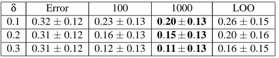
8.1.2 DIABETESDATA
δ Error 100 1000 LOO
0.1 0.32±0.12 0.23±0.13 0.20±0.13 0.26±0.15
0.2 0.31±0.12 0.16±0.13 0.15±0.13 0.20±0.16
0.3 0.31±0.12 0.12±0.13 0.11±0.13 0.16±0.15
Table 2: Bound Methods Compared On Diabetes Data
δ Error 100 1000 LOO Double
0.1 0.070±0.085 0.22±0.11 0.20±0.10 0.27±0.14 0.29±0.17
0.2 0.060±0.074 0.13±0.094 0.12±0.093 0.19±0.14 0.22±0.17
0.3 0.068±0.080 0.084±0.097 0.074±0.096 0.13±0.14 0.18±0.17
Table 3: Bound Methods Compared on Data with a Linear Class Boundary
δ Error 100 1000 LOO Double
0.1 0.18±0.13 0.27±0.15 0.24±0.14 0.31±0.17 0.39±0.12
0.2 0.18±0.12 0.17±0.14 0.16±0.14 0.22±0.17 0.32±0.18
0.3 0.16±0.11 0.12±0.13 0.11±0.13 0.18±0.17 0.28±0.18
Table 4: Bound Methods Compared on Data with a Nonlinear Class Boundary
dimensions. We use t = 200 training examples and w = 15 working examples for each trial. We use 1-nearest neighbor classification.
The error indicates that this is a challenging data set for 1-nearest neighbor classification; even a classifier that always returns the label of the class with 500 examples of the 768 in the data would have average error about 0.35. The bounding method that uses 1000 partitions in a sampled filter performs best for all three values ofδ. On average, that method adds error rate margins of 20% for
δ= 0.1, about 15% forδ= 0.2, and about 11% forδ= 0.3.
8.1.3 DATA WITH ALINEARCLASS BOUNDARY
Table 3 has results for randomly generated data. The data consist of 1100 examples drawn uniformly at random from a three-dimensional input cube with length one on each side. The class label is zero if the input is from the left half of the cube and one if the input is from the right half of the cube. For these tests, there are t = 100 training examples and w = 10 working examples, using 1-nearest neighbor classification. Once again, the method that uses a sample filter with 1000 partitions in the sample outperforms the other methods in the test. On average, the method adds error rate margins of 20% forδ= 0.1, about 12% forδ= 0.2, and about 7.5% forδ= 0.3.
8.1.4 DATA WITH ANONLINEAR CLASSBOUNDARY
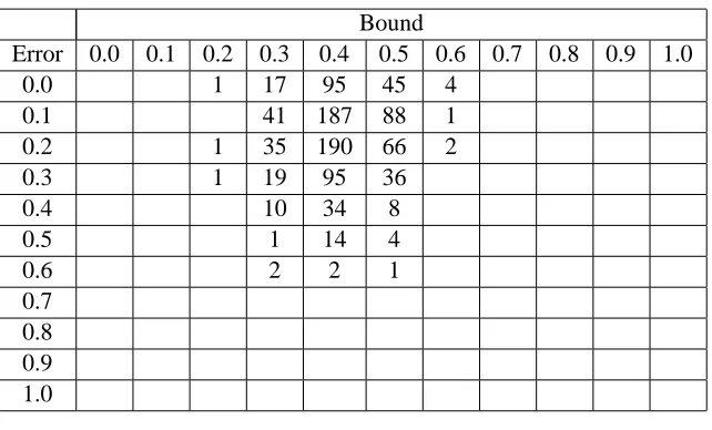
Bound
Error 0.0 0.1 0.2 0.3 0.4 0.5 0.6 0.7 0.8 0.9 1.0
0.0 1 17 95 45 4
0.1 41 187 88 1
0.2 1 35 190 66 2
0.3 1 19 95 36
0.4 10 34 8
0.5 1 14 4
0.6 2 2 1
0.7 0.8 0.9 1.0
Table 5: Bounds vs. Errors forδ= 0.1
error. As in the previous test, the method that uses a sample filter with 1000 partitions in the sample outperforms the other methods in the test. The method adds error rate margins that are higher than for the previous test, that is, about 24% forδ= 0.1, about 16% forδ= 0.2, and about 11% forδ= 0.3.
8.1.5 COMPARISON TOBOUNDSBASED ONVC DIMENSION
The test results in tables 1 to 4 show that error bounds based on worst likely assignments can be effective for small data sets. Compare these bounds to error bounds based on VC dimension (Vapnik and Chervonenkis, 1971), as follows. Suppose that we train linear classifiers on the training sets for our tests. To simplify our analysis, assume that all trained classifiers are consistent, that is, they have zero error on their training data. This consistency assumption produces stronger VC bounds, allowing us to use the bound formula (Cristianini and Shawe-Taylor, 2000, p. 56):
2
t
d log2et d +log
2
δ
,
where t is the number of training examples, d is the VC dimension, which is one more than the number of input dimensions for linear classifiers, andδis the allowed probability of bound failure. Letδ= 0.3. For the iris problem, t = 40 and d = 5, producing bound 1.5. For the diabetes problem,
t = 200, d = 9, and the bound is 0.65. For the problems with randomly generated data, t = 100, d =
4, and the bound is 0.62. Compare these bounds to those forδ= 0.3 in tables 1 to 4.
8.2 Joint Frequencies of Errors and Error Bounds
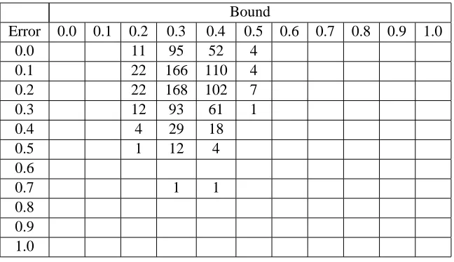
Bound
Error 0.0 0.1 0.2 0.3 0.4 0.5 0.6 0.7 0.8 0.9 1.0
0.0 11 95 52 4
0.1 22 166 110 4
0.2 22 168 102 7
0.3 12 93 61 1
0.4 4 29 18
0.5 1 12 4
0.6
0.7 1 1
0.8 0.9 1.0
Table 6: Bounds vs. Errors forδ= 0.2
Bound
Error 0.0 0.1 0.2 0.3 0.4 0.5 0.6 0.7 0.8 0.9 1.0
0.0 43 87 14
0.1 5 99 200 22 2
0.2 1 96 164 25
0.3 2 56 91 10 1
0.4 2 26 33 4
0.5 5 7 2
0.6 2
0.7 1
0.8 0.9 1.0
Table 7: Bounds vs. Errors forδ= 0.3
Bound Margin
δ <0.0(f ailure) 0.0 (exact) +0.1 +0.2
0.1 3.1% 5.8% 13.8% 26.8%
0.2 6.4% 13.3% 25.1% 28.0%
0.3 11.0% 19.6% 27.3% 26.9%
Table 8: Frequencies of Bound Margins
w 1000 LOO Double 3 0.20±0.16 0.23±0.22 0.073±0.21
4 0.21±0.10 0.27±0.18 0.13±0.25
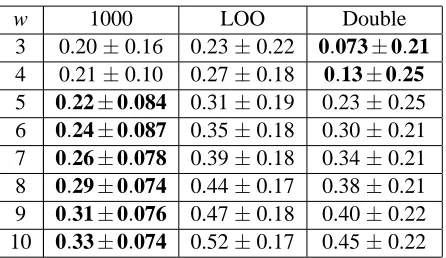
5 0.22±0.084 0.31±0.19 0.23±0.25 6 0.24±0.087 0.35±0.18 0.30±0.21 7 0.26±0.078 0.39±0.18 0.34±0.21 8 0.29±0.074 0.44±0.17 0.38±0.21 9 0.31±0.076 0.47±0.18 0.40±0.22 10 0.33±0.074 0.52±0.17 0.45±0.22 Table 9: Bounds vs. Number of Working Examples forδ= 0.1
Table 8 summarizes the frequencies of bound margins, that is, of differences between bound and error. A bound margin less than zero means the bounding method fails, supplying an invalid error bound. From the failure column in Table 8, observe that the actual frequency of bound failure is significantly less thanδ, the allowed rate of failure. The subsequent columns indicate differences between bound and actual error: exact match, over by 0.1, and over by 0.2.
Suppose we define bound failure as a negative margin and bound success as a valid bound within 0.2 of actual error. Then forδ= 0.1, we have about 3% failure and about 46% success. Forδ= 0.2, we have about 6% failure and about 66% success. Forδ= 0.3, we have 11% failure and about 74% success.
8.3 Working Set Sizes and Bounds
The next results are from tests to explore how working set sizes affect error bounds. In general, since the bounding methods rely on training examples to constrain the set of likely assignments and hence to constrain the error bound, having more training examples and fewer working examples produces stronger bounds. These tests illustrate this effect and compare it over some bounding methods.
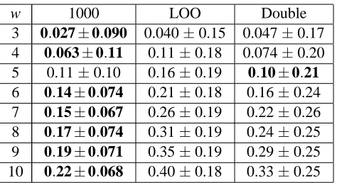
These tests use the iris classification data. The bounding methods are a sampled filter with 1000 sample partitions (1000), virtual partitioning with a leave-one-out filter (LOO), and virtual partitioning with a filter that scores one for each example misclassified by both of its two nearest neighbors (Double). Forδ = 0.1, δ = 0.2, and δ = 0.3, the number of training examples is held constant at t = 40 while the number of working examples w varies from three to 10.
Table 9 shows results forδ = 0.1, with the lowest mean score for a bounding method in each row in bold. Note that the double-error method is better than the other two methods for small working sets, but not for larger ones. Recall that the double-error method is most effective when each working example has as nearest neighbors training examples that agree with one another. As working set sizes increase, it becomes more likely that working examples become nearest neighbors of other working examples, weakening the double-error filter.
Table 10 shows results forδ= 0.2, with the lowest mean score for a bounding method in each row in bold. A variety of methods perform well for small working sets, but the sampled filter method works best for larger working sets.
w 1000 LOO Double 3 0.027±0.090 0.040±0.15 0.047±0.17 4 0.063±0.11 0.11±0.18 0.074±0.20
5 0.11±0.10 0.16±0.19 0.10±0.21
6 0.14±0.074 0.21±0.18 0.16±0.24 7 0.15±0.067 0.26±0.19 0.22±0.26 8 0.17±0.074 0.31±0.19 0.24±0.25 9 0.19±0.071 0.35±0.19 0.29±0.25 10 0.22±0.068 0.40±0.18 0.33±0.25 Table 10: Bounds vs. Number of Working Examples forδ= 0.2
w 1000 LOO Double
3 0.0017±0.024 0.018±0.11 0.040±0.16 4 0.0083±0.045 0.043±0.15 0.057±0.17 5 0.027±0.069 0.068±0.16 0.077±0.17 6 0.047±0.075 0.11±0.18 0.10±0.19 7 0.070±0.075 0.16±0.19 0.14±0.22 8 0.088±0.065 0.20±0.19 0.18±0.23 9 0.11±0.061 0.24±0.20 0.24±0.24 10 0.13±0.064 0.29±0.19 0.27±0.23 Table 11: Bounds vs. Number of Working Examples forδ= 0.3
the sampled filter method improves noticeably asδ increases. In contrast, the performance of the double-error filter does not change much withδ, especially for small working sets.
9. Discussion
This paper introduces a new method to compute an error bound for applying a classifier based on training examples to a set of working examples with known inputs. The method uses information from the training examples and inputs of working examples to develop a set of likely assignments to outputs of the working examples. A likely assignment with maximum error determines the bound. The method is very effective for small data sets.
In the bounds, filters translate training examples and inputs of working examples into constraints on the assignments to outputs of the working examples. Several filters are introduced in this paper. The complete filter is simple and direct; it evaluates each assignment by comparing the error caused by the training/working partition at hand to the errors caused by all other training/working partitions, rejecting the assignment as unlikely if the error for the partition at hand is especially large. The complete filter is effective because it optimizes directly over the error on the partition at hand, which is the basis for the bound. The sampled filter is an easier-to-compute variant that uses only a subset of training/working partitions rather than computing error for all of them. With a sufficient number of samples, the sampled filter performs about as well as the complete filter.
whether assignments are likely. This paper introduces a filter based on leave-one-out error and presents an algorithm based on that filter to efficiently compute an error bound for 1-nearest neigh-bor classification. This paper also introduces a filter based on whether the two nearest neighneigh-bors both misclassify an example. Tests show that this filter can be more effective than the complete filter for problems with little classification error and small numbers of working examples.
Directions for future research include:
1. Develop and analyze new filters for use with virtual partitions, to compete with the leave-one-out and double-error filters presented here.
2. Analyze how training set size, working set size, and properties of the data influence the bounds, with the goal of developing new filters that target different types of problems.
3. Develop efficient algorithms for nearest neighbor classifiers using virtual partitioning with filters beyond the leave-one-out filter.
4. Develop efficient algorithms to compute error bounds using virtual partitioning for classi-fiers other than nearest neighbor classiclassi-fiers, such as condensed and edited nearest neighbors classifiers (Devroye et al., 1996) and support vector machines (Vapnik, 1998).
5. Explore how to use efficient bounds for nearest neighbor classifiers to indirectly produce bounds for other types of classifiers. For example, for support vector machines, first bound nearest neighbor error. Then use the bound to constrain assignments, and bound the support vector machine error by the maximum error over the constrained set of assignments.
6. Consider using alternatives to the set of sister partitions in the complete and sampled filters. For example, with 100 training examples and 10 working examples, partition the training examples into blocks of 10 examples each. Treating the working examples as another block, there are 11 blocks. Each partition that has one block as the working examples and the remaining blocks as the training examples is equally likely. So these partitions can be used in place of the sister partitions. As another example, with 10 training examples and 10 working examples, pair off each working example with a different training example. Each partition that has one of each pair in the working examples and the other in the training examples is equally likely. So these partitions can be used in place of the sister partitions.
Acknowledgments
We thank Joel Franklin for encouraging this research through his example and his teaching. We also thank two anonymous referees for very helpful suggestions on notation and presentation.
Appendix A. Java Code to Compute Error Bounds for 1-Nearest Neighbor Classifiers
public class VirtualPartitionBounder {
Problem p; // Handles examples, labels, neighbors, memberships in T and W. int[][][][] e; // e[i][j][k][y]’s.
int[][] a; // a[i][j]’s to accumulate a slice over children. int[][] b; // b[i][j]’s to accumulate a slice over children.
int[] order; // Ordering of examples with children in F before parents int[][] children; // children[k][] is a list of children of k in F int[] roots; // Examples that are roots in F
/**
* Constructor. **/
public VirtualPartitionBounder(Problem p) {
this.p = p;
this.e = new int[p.sizeT()+1][p.sizeW()+1][p.sizeTuW()][2]; this.a = new int[p.sizeT()+1][p.sizeW()+1];
this.b = new int[p.sizeT()+1][p.sizeW()+1]; }
/**
* Returns a bound on the number of errors on W by T, with probability * of bound failure at most delta.
**/
public int bound(double delta) {
int[][] v = computePossibilities();
double[][] u = computeTails();
int m = 0;
for (int i=0; i<u.length; i++) for (int j=0; j<u[i].length; j++) {
if (u[i][j]>=delta) m = max(m, v[i][j]); }
return m; }
/**
public int[][] computePossibilities() {
computeOrderChildrenAndRoots();
// Compute members order, children, and roots.
clearE(); // Set all e[i][j][k][y] to -1.
// Loop through slices.
for (int i=0; i<order.length; i++) {
int k = order[i];
for (int yk=0; yk<2; yk++) computeSlice(k, yk, children[k]); }
combineRoots(); // Use slices for roots to compute v-values.
return a; }
/**
* Computes a slice e[][][k][yk] by accumulating terms over children. **/
private void computeSlice(int k, int yk, int[] kids) {
clearA(); // Set all a[i][j] to -1. clearB(); // Set all b[i][j] to -1.
// Set intial values in a by treating k as a leaf in F. if (p.inT(k)) // Example k is in T.
{
if (yk!=p.getLabel(k)) return; // Impossible label on k. else a[0][0] = 0; // Correct label on k.
}
else // Example k is in W. {
p.setLabel(k, yk); // Assign label yk to k.
if (p.isMisclassifiedByT(k)) a[0][0] = 1; else a[0][0] = 0;
}
// Accumulate terms over children.
int n = kids[look]; // Get child.
for (int yn=0; yn<2; yn++) // Label child. {
if (p.inT(n) && yn!=p.getLabel(n)) continue; if (p.inW(n)) p.setLabel(n, yn);
int di = p.cT(n,k) + p.dT(n,k); int dj = p.cW(n,k) + p.dW(n,k);
for (int i=0; i<e.length; i++) for (int j=0; j<e[i].length; j++)
if (e[i][j][n][yn]!=-1) {
for (int ii=0; ii<a.length; ii++) for (int jj=0; jj<a[ii].length; jj++)
if (a[ii][jj]!=-1) {
b[ii+i+di][jj+j+dj] = max(b[ii+i+di][jj+j+dj], a[ii][jj] + e[i][j][n][yn]);
} } }
copyBToA(); // Copy b to a before handling the next child. clearB(); // Set all b[i][j] to -1.
}
insertAIntoE(k, yk); }
/**
* Combine roots to compute v-values. Treat each root as a child * of a virtual super-root.
**/
private void combineRoots() {
clearA(); // Set all a[i][j] to -1. clearB(); // Set all b[i][j] to -1.
a[0][0] = 0; // The super-root introduces no errors.
// Accumulate terms over roots.
int n = roots[look]; // Get root.
for (int i=0; i<e.length; i++) for (int j=0; j<e[i].length; j++) {
int v = max(e[i][j][n][0], e[i][j][n][1]);
if (v!=-1)
for (int ii=0; ii<a.length; ii++) for (int jj=0; jj<a[ii].length; jj++)
if (a[ii][jj]!=-1)
b[ii+i][jj+j] = max(b[ii+i][jj+j], a[ii][jj] + v);
}
copyBToA(); // Copy b to a before handling the next root. }
} }
Now consider the storage and time requirements for this technique. The storage is dominated by the array e, which has size O(tw(t+w)). The time is dominated by the nested loops in methods computePossibilities, computeSlice, and combineRoots. Examine the nested loops in computeSlice that run for each child and possible y-value for the child. The nesting is four deep, with two loops of size t+1 and two of size w+1. So, for each child-parent relationship, the time is O(t2w2). Note that the loops for each root in combineRoots are similar to those for each child in computeSlice. Since each of the t+w examples is a child of one example in F or a root in F, and there are at most two possible y-values for each example, the total time is O(t2w2(t+w)).
To reduce storage, discard the slice for each example after using it to compute the slice for the parent of the example in F. To reduce storage and time in most cases, store a list of nonnegative val-ues for each slice rather than storing the slice in array form with all the−1’s included. Then iterate over those lists rather than all pairs (i,j) and (ii,jj) in methods computeSlice and combineRoots.
References
J.-Y. Audibert. PAC-Bayesian Statistical Learning Theory. PhD thesis, Laboratoire de
Probabilities et Modeles Aleatoires, Universites Paris 6 and Paris 7, 2004. URL
http://cermis.enpc.fr/˜audibert/ThesePack.zip.
E. Bax. Partition-based and sharp uniform error bounds. IEEE Transactions on Neural Networks, 10(6):1315–1320, 1999.
A. Blum and J. Langford. Pac-mdl bounds. In Proceedings of the 16th Annual Conference on