On Relevant Dimensions in Kernel Feature Spaces

On Relevant Dimensions in Kernel Feature Spaces

Mikio L. Braun [email protected]

Technische Universit ¨at Berlin Franklinstr. 28/29, FR 6-9 10587 Berlin, Germany

Joachim M. Buhmann [email protected]

Institute of Computational Science ETH Zurich, Universit ¨atstrasse 6 CH-8092 Z¨urich, Switzerland

Klaus-Robert M ¨uller∗ [email protected]

Technische Universit ¨at Berlin Franklinstr. 28/29, FR 6-9 10587 Berlin, Germany

Editor: Peter Bartlett

Abstract

We show that the relevant information of a supervised learning problem is contained up to negligi-ble error in a finite number of leading kernel PCA components if the kernel matches the underlying learning problem in the sense that it can asymptotically represent the function to be learned and is sufficiently smooth. Thus, kernels do not only transform data sets such that good generalization can be achieved using only linear discriminant functions, but this transformation is also performed in a manner which makes economical use of feature space dimensions. In the best case, kernels pro-vide efficient implicit representations of the data for supervised learning problems. Practically, we propose an algorithm which enables us to recover the number of leading kernel PCA components relevant for good classification. Our algorithm can therefore be applied (1) to analyze the interplay of data set and kernel in a geometric fashion, (2) to aid in model selection, and (3) to denoise in feature space in order to yield better classification results.

Keywords: kernel methods, feature space, dimension reduction, effective dimensionality

1. Introduction

Kernel machines implicitly map the data into a high-dimensional feature space in a non-linear fash-ion using a kernel functfash-ion. This mapping is often referred to as an empirical kernel map (Sch ¨olkopf et al., 1999; Vapnik, 1998; M ¨uller et al., 2001; Sch ¨olkopf and Smola, 2002). By virtue of the empir-ical kernel map, the data is ideally transformed in a way such that a linear discriminative function can separate the classes with low generalization error by a canonical hyperplane with large mar-gin. Such large margin hyperplanes provide an appropriate mechanism of capacity control and thus “protect” against the high dimensionality of the feature space.

However, this picture is incomplete as it does not explain why the typical variants of capacity control cooperate well with the induced feature map. This paper adds a novel aspect as the key idea

to this picture. We show theoretically that if the learning problem matches the kernel well, the rele-vant information of a supervised learning data set is always contained in the subspace spanned by a finite and typically small number of leading kernel PCA components (principal component analysis in the feature space induced by the kernel, see below and Section 2), up to negligible error. This re-sult is based on recent approximation bounds for the eigenvectors of the kernel matrix which show that if a function can be reconstructed using only a few kernel PCA components asymptotically, then the same already holds in a finite sample setting, even for small sample sizes.

Consequently, the use of a kernel function not only greatly increases the expressive power of linear methods by non-linearly transforming the data, but it does so ensuring that the high dimen-sionality of the feature space does not become overwhelming: the relevant information for learning stays confined within a comparably low-dimensional subspace. This finding underlines the efficient use of data that is made by kernel machines if the kernel works well for the learning problem. A smart choice of kernel permits to make better use of the available data at a favorable “number of data points per effective dimension”-ratio, even for infinite-dimensional feature spaces. The kernel induces an efficient representation of the data in feature space such that even unregularized methods like linear least squares regression are able to perform well on the reduced feature space.

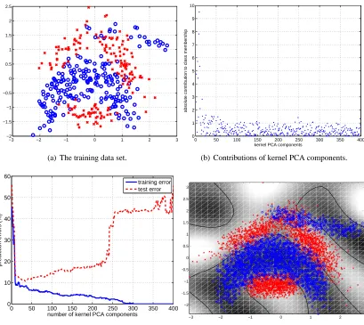
Let us consider an example. Figure 1(a) shows a two-dimensional classification problem (the

banana data set from R¨atsch et al., 2001). We can visualize the contributions of the individual

kernel PCA components1to the class membership by plotting the absolute values of scalar products between the labels and the kernel PCA components. Figure 1(b) shows the resulting contributions sorted by decreasing principal value (variance along principal direction). We can observe that the contributions are concentrated in the leading kernel PCA directions, but a large fraction of the information is contained in the later components as well.

Note, however, that the class membership information in the data set also contains a certain amount of noise. Therefore, Figure 1(b) actually shows a mixture of relevant information and noise. We need to devise a different procedure for assessing the amount of task-relevant information in certain kernel PCA components. This can be accomplished by incorporating a second data set from the same source for testing. One first projects onto the subspace spanned by a number of leading kernel PCA components, trains a linear classifier (for example, by least squares regression) and then measures the prediction error on the test set. The test error is large either if the considered subspace did not capture all of the relevant information, or if it already contained too much noise leading to overfitting. If the minimal test error is on par with a state-of-the-art method independently trained using the same kernel then the subspace has successfully captured all of the relevant information.

If we apply this procedure to our data set, we obtain training and test errors as shown in Fig-ure 1(c). By definition, the training error decreases as more and more dimensions are used. How-ever, after decreasing quickly initially, the test error eventually starts to increase again. The minimal test error also coincides with the actually achievable test error using, for example, support vector machines. Therefore, we see that the later components only contain noise, and the relevant infor-mation is contained in the leading kernel PCA components. In this paper, our goal is to understand

−3 −2 −1 0 1 2 3 −2 −1.5 −1 −0.5 0 0.5 1 1.5 2 2.5

(a) The training data set.

0 50 100 150 200 250 300 350 400 0 1 2 3 4 5 6 7 8 9 10

kernel PCA components

a b s o lu te c o n tr ib u ti o n t o c la s s m e m b e rs h ip

(b) Contributions of kernel PCA components.

0 50 100 150 200 250 300 350 400

0 10 20 30 40 50 60

number of kernel PCA components

prediction errors (%)

training error test error

(c) Training and test errors using only leading kernel PCA components.

−3 −2 −1 0 1 2

−2 −1.5 −1 −0.5 0 0.5 1 1.5 2 2.5 3

(d) The solution on the test data set.

Figure 1: A more complex example (resample 1 of the “banana” data set, see Section A). This time, the information is not contained in a single component. Nevertheless, the test error of a

hyperplane learned using only the first d components has a clear minimum at d=34 at

optimal error rate (cf. Table 3), showing that the relevant information is contained in the leading 34 directions.

more thoroughly why and when this effect occurs, and to estimate the dimensionality of a concrete data set given a kernel.

the relevant information. Components which contain only little variance will therefore not contain relevant information. If such a component manages to contribute much to the label information, it will only reflect noise.

What practical implications follow from these results? We explore several possibilities of using these ideas to assess the suitability of a kernel or a family of kernels to a specific data set. The main idea is that the observed dimensionality of the data set in feature space is characteristic for the relation between a data set and a kernel. Roughly speaking, the relevant dimensionality of the data set corresponds to the complexity of the learning problem when viewed through the “lens” of the kernel function. Using the estimated dimensionality, one can project the labels onto the corresponding subspace and obtain a noise free version of the labels. By comparing the denoised labels to the original labels, one can estimate of the amount of noise contained in the labels. One therefore obtains a more detailed measure of the fit between the kernel and the data set as compared to, for example, the cross-validation error alone. This allows us to take a closer look at data sets on which the achieved error is quite large. In such cases, we are able to distinguish whether the data set is highly complex and the amount of data is insufficient, or the amount of intrinsic noise is very large. This is practically relevant as one has to deal with both these cases quite differently, either by providing more data, or by thinking about means to obtain less noisy or ambiguous features.

We summarize the main contributions of this paper: (1) We provide theoretical bounds showing that the relevant information (defined in Section 2) is actually contained in the leading projected kernel principal components under appropriate conditions. (2) We propose an algorithm which es-timates the relevant dimensionality and related eses-timates of the data set and permits to analyze the appropriateness of a kernel for the data set, and thus to perform model selection among different ker-nels. (3) We validate the accuracy of the estimates experimentally by showing that non-regularized methods perform on the reduced feature space on par with state-of-the-art kernel methods. We ana-lyze some well-known benchmark data sets in Section 5. Note that we do not claim to obtain better performance within our framework when compared to, for example, cross-validation techniques. Rather, we are on par. Our contribution is to foster an understanding about a data set and to gain better insights of whether a mediocre classification result is due to intrinsic high dimensionality of the data (and consequently insufficient number of examples), or an overwhelming noise level.

2. Preliminaries

Let us start to formalize the ideas introduced so far. As usual, we consider a data set (X1,Y1), . . . ,(Xn,Yn)where the inputs X lie in some space

X

Y

{±1_} for classification or

Y

irrespective of whether we are considering a classification or regression task. We assume that the

(Xi,Yi)are drawn i.i.d. from some probability measure P_X×Y. In kernel methods, the data is

non-linearly mapped into some feature space

F

F

computed by the kernel k in closed form: hΦ(x),Φ(x0)_i=k(x,x0). Summarizing all the pairwise scalar products results in the (normalized) kernel matrix K with entries k(Xi,Xj)/n.

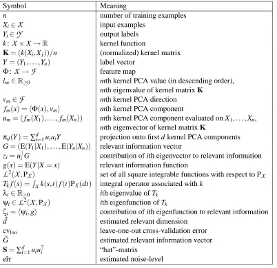
In the discussion below, we study the relationship between the label vector Y = (Y1, . . . ,Yn)and

Symbol Meaning

n number of training examples

Xi∈

X

Yi∈

Y

k :

X

X

K= (k(Xi,Xj))/n (normalized) kernel matrix

Y = (Y1, . . . ,Yn) label vector

Φ:

X

F

lm∈R≥0 mth kernel PCA value (in descending order),

mth eigenvalue of kernel matrix K

vm_∈

F

fm(x) =hΦ(x),vmi mth kernel PCA component

um= (fm(X1), . . . ,fm(Xn)) mth kernel PCA component evaluated on X1, . . . ,Xn, mth eigenvector of kernel matrix K

πd(Y) =∑di=1uiuiY projection onto first d kernel PCA components

G= (E(Y1|X1), . . . ,E(Yn|Xn)) relevant information vector

zi=u>iG contribution of ith eigenvector to relevant information

g(x) =E(Y_|X=x) relevant information function

L

X

X) set of all square integrable functions with respect to PX

Tkf(s) =

R

Xk(s,t)f(t)PX(dt) integral operator associated with k

λi∈R≥0 ith eigenvalue of Tk

ψi∈

L

X

ζi=hψi,gi contribution of ith eigenfunction to relevant information

ˆ

d estimated relevant dimension

cvloo leave-one-out cross-validation error

ˆ

G estimated relevant information vector

S=∑d

i=1uiu>i “hat”-matrix

ˆ

err estimated noise-level

Table 1: Overview of notation used in this paper.

with the vectors directly, the principal directions are represented using the points Xi of the data set:

vm=

n

∑

i=1

αiΦ(Xi),

whereαi= [um]i/lm,[um]iis the ith component of the mth eigenvector of the kernel matrix K, and lmthe corresponding eigenvalue.2 Still, vm can usually not be computed explicitly such that one

instead works with kernel PCA components

fm(x) =_hΦ(x),vm_i.

We are interested in the relation between fmand a label vector Y . As we have seen in the

introduc-tion, it seems that only a finite number of leading kernel PCA components are necessary to represent the relevant information about the learning problem up to a small error.

Therefore, we would like to compare fmwith the values Y1, . . . ,Ynat the points X1, . . . ,Xn. The

following easy lemma summarizes the relationship between the sample vector of fmand Y .

Lemma 1 The mth kernel PCA component fmevaluated on the Xis is equal to the mth eigenvector of

the kernel matrix K: (fm(X1), . . . ,fm(Xn)) =um. Consequently, the sample vectors are orthogonal,

and the projection of a vector Y_∈Rnonto the leading d kernel PCA components is given byπd(Y) =

∑d

m=1umu>mY.

Proof The mth kernel PCA component for a point Xj in the training set is

fm(Xj) =hΦ(Xj),vmi=

1

lm n

∑

i=1

hΦ(Xj),Φ(Xi)i[um]i=

1

lm n

∑

i=1

k(Xj,Xi)[um]i.

The sum computes the jth component of Kum, and Kum=lmum, because umis an eigenvector of K.

Therefore

fm(Xj) = 1

lm

[lmum]j= [um]j.

Since K is a symmetric matrix, its eigenvectors umare orthonormal, and the projection of Y onto

the space spanned by the first d kernel PCA components is given by∑d_m=1umu>_mY .

Since the kernel PCA components are orthogonal, the coefficients of a vector Y _∈Rn _with

respect to the basis u1, . . . ,unis easily computed by forming the scalar products. We call the

coeffi-cients

zm=u>_mY (1)

of Y w.r.t. the basis formed from the kernel PCA components the kernel PCA coefficients. They are the central object of our discussion.

The projection of Y to a kernel PCA component can be thought of as the least squares regression of Y using only the direction along the kernel PCA component in feature space.

Using the kernel PCA coefficients, we can extend the projected labels to new points via

ˆ

Y(x) =

d

∑

m=1

zmfm(x),

which amounts to the prediction of least squares regression on the reduced feature space.

3. The Label Vector and Kernel PCA Components

−3 −2 −1 0 1 2 3 4 5 −1

−0.8 −0.6 −0.4 −0.2 0 0.2 0.4 0.6 0.8 1

X

Y

d a ta

re le v a n t in fo rm a tio n G p (x | Y = 1) p (x | Y = −1)

−4 −3 −2 −1 0 1 2 3 4

−0.4 −0.2 0 0.2 0.4 0.6 0.8 1 1.2

X

Y

d a ta

re le v a n t in fo rm a tio n G

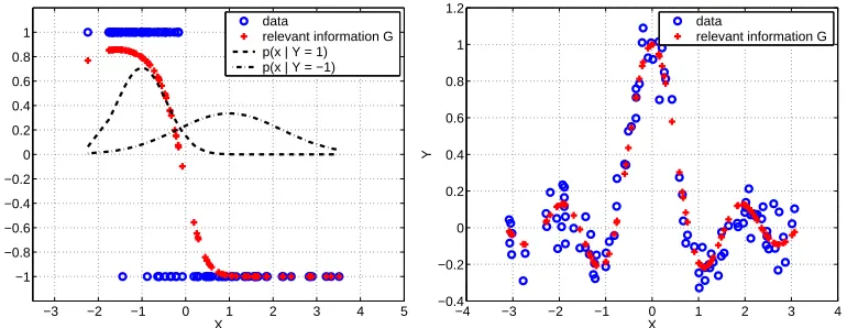
Figure 2: Relevant information vectors visualized for the classification and the regression case. In the (two-class) classification case (left) it encodes the posterior probability (scaled between ₋1 and 1), in the regression case it is the sample vector of the function to be learned.

3.1 Decomposing the Label Vector Information

We start the discussion by defining formally what the relevant information contained in the labels is. Given a label vector Y , we define the relevant information vector as the vector of the expected labels:

G= (E(Y1|X1), . . . ,E(Yn|Xn)).

Intuitively speaking, G is a noise-free version of Y . This vector contains all the relevant information about the outputs Y of the learning problem: For regression, G amounts to the values of the true function. For the case of two-class classification, the vector G contains all the information about the optimal decision boundary. Since E(Y_|X) =P(Y=1_|X)₋P(Y=₋1_|X), the sign of G contains the relevant information on the true class membership by telling us which class is more probable (see Figure 2 for examples). Thus, using this denoised label information, the learning problem becomes much easier as the denoised labels already contain the Bayes optimal prediction at that point.3

Using G we obtain a very useful additive decomposition of the labels into “signal” and “noise”:

Y =G+N.

In this setting, we are now interested in showing that G is contained in the leading kernel PCA com-ponents, such that projecting G onto the leading kernel PCA components leads to only negligible error. In the following, we treat the signal and noise part of Y separately. This is possible because the projectionπdis a linear operation such thatπd(Y) =πd(G+N) =πd(G) +πd(N).

3.2 The Relevant Information Vector

We first treat the relevant information vector G. The location of G with respect to the kernel PCA components is characterized by scalar products with the eigenvectors of the kernel matrix. We start by discussing this relationship in an asymptotic setting and then transfer the results back to the finite sample setting using convergence results for the spectral properties of the kernel matrix

Using the kernel function k, we define the integral operator

Tkf(s) =

Z

Xk(s,t)f(t)PX(dt),

where PX is the marginal distribution which generates the inputs Xi. It is well known that the linear

operator

˜

Tkf(s) =

1

n n

∑

i=1

k(s,Xi)f(Xi)

represented by the kernel matrix approximates Tkas the number of points tend to infinity (see, for

example, von Luxburg, 2004). While this follows easily for a fixed f and s, making the argument theoretically exact for operators (this means uniform over all functions) is not trivial.

As a consequence, the eigenvalues and eigenvectors of ˜Tk, which are equal to those of the kernel matrix, converge to those of Tk(see Koltchinskii and Gin´e, 2000; Koltchinskii, 1998). In particular,

scalar products of sample functions and eigenvectors of K converge to scalar products with eigen-functions of Tk. The asymptotic counterpart of the relevant information vector G is the function

g(x) =E(Y_|X=x).

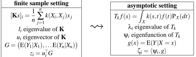
These correspondences are summarized in Figure 3. In summary, we can think of zi=u>iG (properly

scaled) as an approximation toζi=hψi,gi.

finite sample setting

[Kx]i=

1

n n

∑

j=1

k(Xi,Xj)xj

lieigenvalue of K uieigenvector of K

G= E(Y1|X1), . . .E(Yn|Xn)

zi=u>iG

asymptotic setting

Tkf(s) =

Z

Xk(s,t)f(t)PX(dt)

λieigenvalue of Tk

ψi eigenfunction of Tk g(x) =E(Y_|X=x)

ζi=hψi,gi

Figure 3: Transition from the finite sample size and asymptotic setting.

In the asymptotic setting, it is now fairly easy to specify conditions such that g is contained in the subspace spanned by a finite number of leading eigenfunctions ψi. Since it is unrealistic that g is exactly contained in a finite dimensional subspace, we relax that requirement and instead only

require thatζidecays to zero at the same rate as the eigenvalues of Tk.

A natural assumption is that the learning problem can be asymptotically represented by the given kernel function k. By this we mean that there exists some function h_∈

L

X

g=Tkh. Using the spectral decomposition of Tk, this implies

g=Tkh=

∞

∑

i=1

λihψi,hiψi. (2)

Since the sequence ofαi=hψi,hiis square summable, it follows that

ζi=hψi,gi=λiαi=O(λi).

Intuitively speaking, (2) translates to asymptotic representability of the learning problem: As n_→∞, it becomes possible to represent the optimal labels using the kernel function k.

Furthermore, we assume that k is bounded. This technical requirement is mainly necessary to ensure that g is also bounded. The requirement holds for common radial basis function kernels like the Gaussian kernel, and also if the underlying space

X

Note that the requirement that g lies in the range of Tk is essential. If this is not the case, we

cannot expect that the scalar products decay at a given rate. Also note that it is in fact possible to break this condition. For example, if k is continuous, every non-continuous function does not lie in the range of Tk.

The question is now whether the same behavior can be expected for a finite data set. This question is not trivial, because eigenvector stability is known to be linked to the gap between the corresponding eigenvalues, which is fairly small for small eigenvalues (see, for example, Zwald and Blanchard, 2006).

The main theoretical result of this paper (Theorem 1 in the Appendix) provides a bound of the form

1

n|u

>

iG| ≤liC+E

which expresses an essential equivalence between the finite sample setting and the asymptotic set-ting with two modifications: The decay rate O(λi)of the scalar productshψi,giholds for the finite

sample up to a (small) additive error E withλireplaced by its finite sample approximation li.

The technical details of this theorem and the proof are deferred to the appendix. Let us discuss how the absolute term occurs in the bound and why it can be expected to be small. An exact scaling bound (without additive term E) can only be derived (at least following the approach taken in this paper) for the case where the kernel function is degenerate, that is, Tkhas only finitely many

non-zero eigenvalues. The same finiteness restriction also holds for the expansion of g in terms of the eigenfunctions of Tk. The proof thus contains a truncation step of general kernels and general

functions g, leading to a scaling bound on the scalar product and an additive term arising from the truncation. However, as the name suggests, the truncation error E can be made arbitrarily small by considering approximations with many non-zero eigenvalues. At the same time, considering such kernels with more terms in the expansion leads to a larger constant C in the actual scaling part. Thus, both terms have to be balanced by the order of truncation, which permits to control the additive term well practically.

In view of our original concern, the bound shows that the relevant information vector G (as introduced in Section 2) is contained in a number of leading kernel PCA components up to a neg-ligible error. The number of dimensions depends on the asymptotic coefficientsαi and the decay

rate of the asymptotic eigenvalues of k. Since this rate is related to the smoothness of the kernel function, the dimension is small for smooth kernels whose leading eigenfunctionsψi permit good

approximation of g.

3.3 The Noise

To study the relationship between the noise and the eigenvectors of the kernel matrix, no asymptotic arguments are necessary. The key insight is that the eigenvectors are independent of the noise in the labels, such that the noise vector N is typically evenly distributed over all coefficients u>_iN: Let U be

the matrix whose ith column is equal to ui. The coefficients of N with respect to the eigenbasis of K

are then given by U>N. Note that since U is orthogonal, multiplication by its transpose amounts to

a (random) rotation. In particular, this rotation is independent of the noise N as the uidepend on the X s only. Now if the noise has a spherical distribution, for example, N is normally distributed with

covariance matrixσ2_εI, it follows that U>N_∼

N

εI). For heteroscedastic noise in a regression

setting, or for classification, this simple analysis is not sufficient. In that case, the individual u>_iN

are no longer uncorrelated. However, because of the independence of the Ni, the variance of u>iN is

upper bounded by

Var(u>_iN) =

n

∑

j=1

u2_i,jVar(Nj)≤ max

1≤j≤nVar(Nj)

since∑n_j=1u2_i,j =_kuik2=1. Therefore, the variance of the u>iN is not concentrated in any single

coefficient as the total variance does not increase by rotating the basis and the individual variances are bounded by the maximum individual variance before the rotation.

The practical relevance of these observations is that the relevant information and noise part have radically different properties with respect to the kernel PCA components, allowing us to practically estimate the number of relevant dimension for a given kernel and data set. In the next section, we will propose two different algorithms for this task.

4. Relevant Dimension Estimation and Related Estimates

We have seen that the number of leading kernel PCA components necessary to capture the relevant information about the labels of a finite size data set is bounded under the mild assumptions that the learning problem can be represented asymptotically and the kernel is smooth such that the eigenval-ues of the kernel matrix decay quickly. The actual number of necessary dimensions depends on the interplay between kernel and learning data set, giving insights into the suitability of the kernel. For example, a kernel might fail to provide an efficient representation of the learning problem, leading to an embedding requiring many kernel PCA components to capture the information on Y . Or, even worse, a kernel might completely fail to model some part of the learning problem, such that a part of the information appears to be just noise. Therefore, in order to make practical use of the presented insights, we need to devise a method to estimate the number of relevant kernel PCA components for a given concrete data set and choice of kernel.

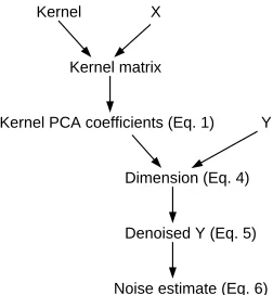
onto the respective subspace and obtain an estimate for the relevant information vector G. By comparing the denoised labels with the original labels, one can then estimate the overall noise level of the data source. Based on these estimates, we discuss how to use the dimensionality estimate for model-selection and to further analyze data sets which so far show inferior performance. Figure 4 summarizes the information flow for the different estimates.

Y Kernel matrix

X Kernel

Noise estimate (Eq. 6) Dimension (Eq. 4) Kernel PCA coefficients (Eq. 1)

Denoised Y (Eq. 5)

Figure 4: Information flow for the estimates.

4.1 Relevant Dimension Estimation (RDE)

The most basic estimate is the number of relevant kernel PCA components. We also call this number simply the relevant dimension or the dimensionality (also see the discussion in Section 6.3). Recall that we have decomposed the labels into Y =G+N , with Gi=E(Yi_|Xi)(see Section 3.1). This decomposition carries over to the kernel PCA coefficients zi =u>iY =u>iG+u>iN. We want to

estimate ˆd such that_|u>_iG_|is negligible for i>d.ˆ

We propose two algorithms for solving this relevant dimension estimation (RDE) task which are based on different approaches to the problem but lead to comparable performance. The first algorithm fits a parametric model to the kernel PCA coefficients, while the second one is based on leave-one-out cross-validation.

4.1.1 RDE BYFITTING ATWO-COMPONENTMODEL(TCM)

The first algorithm works only on the coefficients zi =u>iY . Recall that U is the matrix whose

columns are the eigenvectors of the kernel matrix ui such that z=U>Y =U>G+U>N=G˜+N.˜

In Section 3, we have seen that both parts have significantly different structure. From Theorem 1, we know that_|Gi˜ _{| ≈}O(li), and that the ˜Giare close to zero for all but a leading number of coeffi-cients. On the other hand, as discussed in Section 3.3, the transformed noise ˜N is typically evenly

distributed over all coefficients. Thus, the coefficients of the noise have the shape of an evenly distributed “noise floor” ˜Ni from which the coefficients ˜Gi of the relevant information arise (see Figure 1(b) for an example).

The idea is now to find a cut-off point such that the coefficients are divided into two parts

z1, . . . ,zd and zd+1, . . . ,znsuch that the first part contains the relevant information and the latter part

individual variances

zi_∼

(

N

1) 1≤i≤d,

N

2) d<i≤n.

Of course, in order to be able to extract meaningful information, it should hold that σ1 σ2.

Alternatively, one could assume that zi∼

N

the exact same choice of d.

For real data, both parts need not be actually Gaussian distributed. However, due to lack of additional a priori knowledge on the signal or the noise, the Gaussian distribution represents the optimal choice among all distributions with the same variance according to the maximum entropy principle (Jaynes, 1957).

The negative log-likelihood is proportional to

−log`(d)_∼ d

nlogσ

2 1+

n₋d

n logσ

2

2, with σ21=

1

d d

∑

i=1

z2_i,σ2 2=

1

n−d

n

∑

i=d+1

z2_i. (3)

The estimated dimension is then given as the maximum likelihood fit

ˆ

d=argmin

1≤d≤n0

(₋log`(d)) =argmin

1≤d≤n0

d

nlogσ

2 1+

n₋d

n logσ

2 2

. (4)

Due to numerical instabilities of kernel PCA components corresponding to small eigenvalues, the choice of d should be restricted to 1_≤d_≤n0<n: The coefficients ziare computed by taking scalar

products with eigenvectors ui. For small eigenvalues (small meaning of the order of the available

numerical precision, for double precision floating point numbers, this is typically around 10−16), individual eigenvectors cannot be computed accurately, although the space spanned by all these eigenvectors is accurate. Therefore, coefficients zifor large i are not be reliable. To systematically

stabilize the algorithm, one should therefore limit the range of possible effective dimensions. We have found the choice of 1_≤d_≤n/2 to work well as this choice ensures that at least half of the coefficients are interpreted as noise. For very small and very complex data sets, this choice might prove suboptimal and better thresholds based, for example, on the actual decay of eigenvalues might be advisable. However, on all data sets discussed in this paper, the above choice performed very well.

4.1.2 RDE BYLEAVE-ONE-OUT CROSS-VALIDATION(LOO-CV)

We propose a second algorithm which is based on cross validation, a more general concept than parametric noise modeling. This algorithm only depends on our theoretical results to the extent that it searches for subspaces spanned by leading kernel PCA components. We later compare the two methods to see whether our assumptions were justified.

As stated in Lemma 1, the projection of Y onto the space spanned by the d leading kernel PCA components is given by∑d_i=1uiu>iY , where uiare the eigenvectors of the kernel matrix. The matrix

S=∑d

i=1uiu>i can be interpreted as a “hat matrix” in the context of regression.4 The idea is now to

choose the dimension which minimizes the leave-one-out cross-validation error. This subspace then captures all of the relevant information about Y without overfitting.

Computationally, note that one can write the squared error leave-one-out cross-validation in closed form, similar to kernel ridge regression (see Wahba, 1990):

cvloo(d) =1

n n

∑

i=1

[SY]i−Yi

1₋Sii

2

.

It is possible to organize the computation in a way such that given the eigendecomposition of K, each value cvloo(d)can be computed in O(n)(instead of O(n2)if one naively implements the above

formula): Note that Siiis equal to∑dj=1(uj)2i, therefore, one can compute Siiiteratively by

S0_ii←0

Sd_ii+1_←Sd_ii+ (ud+1)2i.

In the same way, since ˆY=SY =∑d

j=1uju>jY , we get that

ˆ

Y0_←0

ˆ

Yd+1_←Yˆd+ud+1u>d+1Y.

The squared error is in principle not the most appropriate loss function for classification problems. But as we will see below, it nevertheless works well also for classification problems.

4.2 Denoising the Labels and Estimating the Noise Level

One direct application of the dimensionality estimate is the projection of Y onto the first ˆd kernel

PCA components. By Lemma 1, this projection is

ˆ

G0=

ˆ

d

∑

i=1

uiu>_iY.

Then, an estimate of the noiseless labels is given by

ˆ

G=

(

sign ˆG0 classification against_±1 labels ˆ

G0 regression . (5)

Note that this amounts to computing the in-sample fit using kernel principal component regression (kPCR).

The estimated dimension can also be used to estimate the noise level present in the data set by

ˆ err=1

n n

∑

i=1

L(_Yiˆ_{,Yi), (6)}

where L is the loss function.

The accuracy of both these estimates depends on a number of factors. Basically, the estimation error is small if the first ˆd kernel PCA components capture most of G and ˆd is small such that

most of the noise is removed. Note that our assumption that the kernel suits the data set is crucial for both these requirements. If g does not lie in the span of the associated integral operator Tk,

10−5 100 105 0 0.1 0.2 0.3 0.4 0.5 0.6 0.7 kernel width e s t. n o is e l e v e l (% ) dimension (%) noise level

(a) Classification (“banana” data set)

10−6 10−4 10−2 100 102 104 106

0 0.05 0.1 0.15 0.2 0.25 0.3 0.35 0.4 0.45 0.5 kernel width e s t. n o is e l e v e l (M S E ) dimension (%) noise level

(b) Regression (noisy sinc function)

Figure 5: Dimensions and estimated noise levels for varying kernel widths are not suited for model selection as it is unclear how to combine both estimates and they become instable for very small kernel widths. Shown are the 10%, 25%, 50%, 75%, and 90% percentiles over 100 resamples. Legend: “dimension (%)”—estimated dimensionality divided by number of samples. “noise level”—estimated noise level using the`1-norm for classification, and

the (unnormalized)`2-norm for regression.

4.3 Applications to Model Selection

A highly relevant problem in the context of kernel methods is the selection of a kernel from a number of possible candidates which fits the problem best. This problem is usually solved by extensive cross-validation.

We would like to discuss possibilities to use the estimates introduced so far for model selection. Choosing the model based on either dimensionality or noise level alone is not sufficient, since one wants to optimize a combination of both. However, as the two terms live on quite different scales, it is unclear how to combine them effectively. Furthermore, as we will see below, both estimates alone become unstable for very small or very large kernel widths. The log-likelihood which achieves the optimum in (4) overcomes both problems and can be used for effective model selection.

Let us first discuss how the relation between the scale of the kernel and the data set can affect the dimensionality of the embedding in feature space. The standard example for a family of kernels with a scale parameter is the rbf-kernel (also known as Gaussian kernel, see Appendix A). Figure 5 shows the dimension and noise level estimates for a classification data set (the “banana” data set), and a regression data set (the “noisy sinc function” with 100 data points for training, and 1000 data points for testing) over a range of kernel widths. Generally speaking, if the scale of the kernel is too coarse for the problem, the problem tends to appear to be very low-dimensional with a large amount of noise. On the other hand, if the scale of the kernel is too fine the learning problem appears to be very complex with almost no noise.

10−5 100 105 0

0.1 0.2 0.3 0.4 0.5 0.6 0.7 0.8 0.9

kernel width

te

s

t

e

rr

o

r

(%

)

log−lik. (scaled) test error

(a) Classification (“banana” data set)

10−6 10−4 10−2 100 102 104 106

0 0.05 0.1 0.15 0.2 0.25 0.3 0.35 0.4 0.45

kernel width

te

s

t

e

rr

o

r

(M

S

E

)

log−lik. (scaled) test error

(b) Regression (noisy sinc function)

Figure 6: Comparison of test errors and the negative log-likelihood from Equation (3) shows that the negative log-likelihood is highly correlated with the test error and can thus be used for model selection. Shown are the 10%, 25%, 50%, 75%, and 90% percentiles over 100 resamples. Legend: “log-lik. (scaled)”—log-likelihood (scaled). “test error”—test error using the`1-norm for classification, or the (unnormalized)`2-norm for regression.

with respect to the classification and least squares error. We see that the estimated log-likelihoods can be estimated well over the whole range, and that the likelihoods are highly correlated with the actual test error. Thus, the log-likelihood is a reliable indicator for the test errors based on the best separation between signal and noise.

Another alternative, which is somewhat more straight-forward, but conceptually also less inter-esting, is to use the leave-one-out cross-validation error. This quantity also measures how well the kernel can separate the noise from the relevant information, and is directly linked to the test error on an independent data set. We validate both model selection approaches experimentally in Section 5.

4.4 Applications to Data Set Assessment

When working on a concrete data set in a kernel setting, one is faced with the problem of finding a suitable kernel. This problem is usually approached with a mix of hard-won experience and domain knowledge. The main tool for guiding the search are prediction performance measures, the classical one being prediction accuracy. Measurements like the ROC (receiver-operator-curve), or the AUC (area-under-the-curve) give more fine-grained measurements of prediction quality, in particular in areas where many false positives or false negatives are not acceptable.

If, after testing a number of sensible candidates, the achieved prediction quality is satisfying, this approach is perfectly adequate, but more often than not, prediction quality is not as good as desirable. In such a case, it is important to identify the cause for the inferior performance. In principle, three alternatives are possible:

1. The kernels which have been used so far are not suited for the problem.

data set RDE method dimension noise-level

complex data set TCM 50 16.07%

LOO-CV 25 40.59%

noisy data set TCM 9 40.71%

LOO-CV 9 40.71%

Table 2: Estimated dimensions for the two data sets from Figure 7. Methods are “TCM” for RDE by fitting a two-component model, “LOO-CV” for RDE by leave-one-out cross-validation. “noise-level” is measured as normalize mean square error (see Appendix A).

3. Better performance cannot be achieved since the learning problem is intrinsically noisy.

Each of these alternatives requires different approaches. In the first case, a better kernel has to be devised, in the second case, more data has to be acquired, and in the last case, one can either stop searching for a better kernel, or try to improve the quality of the data or the features used.

Ultimately, these questions cannot be answered without knowledge of the true distribution of the data, but the important observation here is that performance measures do not provide enough information to distinguish these cases.

The estimates introduced so far can now be used to obtain evidence for distinguishing between the second and third case. On the one hand, the dimensionality of the problem is related to the complexity of the problem, while the noise level measures the inherent noise. Note that both these estimates depend on the chosen kernel.

Consider the following example: We study two data sets, a simple data set built from a noisy sinc function, and a complex data set based on a high-frequency sine function (see Figure 7). For the same number of data points n=100, both data sets lead to comparable normalized test errors5for the best model selected (A normalized test error of 43.7% on the complex data set and 44.4% on the noisy data set using kernel ridge regression with model selection by leave-one-out cross-validation. Widths were selected from 20 logarithmically spaced points from 10−6to 102, regularization con-stant was selected from 10 logarithmically spaced points from 10−6 to 103). However, the reason for the large error on the complex data set is clearly due to the small number of samples. If we increase the data set size to 1000 points, the normalized test error becomes 2.4%.

The question is now whether we can distinguish these two cases based on the kernel PCA coeffi-cients. In fact, even on visual inspection, the kernel PCA coefficients display significant differences (see Figures 7(c) and 7(d)). We estimate the effective dimension and the resulting noise-level using the two methods we have proposed, the results are shown in Table 2. While both methods lead to different estimates, they both agree on the fact that the noisy data set has comparably low complex-ity and high noise, while the complex data set is quite high-dimensional, in particular if one takes into account that the data set contains only 100 data points. In fact, the RDE analysis on the larger complex data set with 1000 data points gives a dimension of 142, and a noise-level of 1.96%. Thus, the RDE measure correctly indicates that the large test error is due to the insufficient amount of data in the one case, and due to the large noise level in the other case.

This simple example demonstrates how the RDE measure can provide further information be-yond the error rates. Below, we discuss this approach for several benchmark data sets.

−4 −3 −2 −1 0 1 2 3 4 −1.5

−1 −0.5 0 0.5 1 1.5

Normalized Test Error: 43.73%

test points predicted function training points

(a) A complex data set.

−4 −3 −2 −1 0 1 2 3 4 −1.5

−1 −0.5 0 0.5 1 1.5 2

Normalized Test Error: 44.37%

test points predicted function training points

(b) A noisy data set.

0 10 20 30 40 50 60 70 80 90 100

0 0.2 0.4 0.6 0.8 1 1.2 1.4 1.6 1.8 2

kernel PCA components

absolute value of scalar product

kernel width 0.001000

(c) Kernel PCA coefficients for the complex data set.

0 10 20 30 40 50 60 70 80 90 100

0 0.5 1 1.5 2 2.5

kernel PCA components

absolute value of scalar product

kernel width 5.000000

(d) Kernel PCA coefficients for the noisy data set.

Figure 7: For both data sets, the X values were sampled uniformly between₋πandπ. For the com-plex data set, Y =sin(35X) +εwhereεhas mean zero and variance 0.01. For the noisy data set, Y =sinc(X) +ε0whereε0 has mean zero and variance 0.09. Errors are reported as normalized mean squared error (see Appendix A). Below, the kernel PCA coefficients (scalar products with eigenvectors of the kernel matrix) for the optimal kernel selected based on the RDE (TCM) estimates are plotted. Coefficients are sorted by decreasing corresponding eigenvalue.

5. Experiments

5.1 Benchmark Data Sets

We performed experiments on the classification data sets from R¨atsch et al. (2001). For each of the data sets, we analyze it using a family of rbf kernels (see Appendix A). The kernel width is selected automatically using the achieved log-likelihood as described above. The width of the rbf kernel is selected from 20 logarithmically spaced points between 10−2and 104for each data set.

Table 3 shows the resulting dimension estimates using both RDE methods, with the cross-validation based RDE method being slightly biased towards higher dimensions. We see that both methods perform on par, which shows that the strong structural prior assumption underlying RDE is justified.

To assess the accuracy of the dimensionality estimate, we compare an unregularized least-squares fit in the reduced feature space (RDE+kPCR) with kernel ridge regression (KRR) and sup-port vector machines (SVM) on the original data set. The resulting test errors are also shown in Table 3. Note that the combination of RDE and kPCR is conceptually very similar to the kernel projection machine (Vert et al., 2005) which also produces comparable results. However, in that pa-per, no practical method for estimating the dimension (beyond cross-validation) has been proposed. From the resulting test errors, we see that a relatively simple method on the reduced features per-forms on par with the state-of-the-art competitors. We conclude that the identified reduced feature space really contains all of the relevant information. Also note that the estimated noise levels match the actually observed error rates quite well, although there is a slight tendency to under-estimate the true error.

As discussed in Section 4.4, while the test errors only suggest a linear ordering of the data sets by increasing difficulty, using the dimension and noise level estimates, a more fine-grained analysis is possible. We can roughly divide the data sets into four classes (see Table 4), depending on whether the dimensionality is small or large, and the noise level is low or high. Data sets with small noise level show good results, almost irrespective of the dimensionality. The data set image seems to be particularly noise free, given that one can achieve a small error in spite of the large dimensionality.

The data sets breast-cancer, diabetes, flare-solar, german, and titanic, which all have test errors of 20% or more, have only moderately large dimensionalities. This means that the complexity of the underlying optimal decision boundary is not overly large (at least when viewed through the lens of the kernel), but a large inherent noise level prevents better results. Since this holds for rbf-kernels over a wide range of kernel widths, these results can be taken as a strong indicator that the Bayes error is in fact large.

The splice data set seems to be a good candidate for improvement. The noise level is moderately high, while the dimensionality with respect to the rbf-kernel seems quite high. We would like to use our dimensionality and noise level estimate as a tool to examine different kernel choices. (See Section C for further details).

data set TCM LOO-CV TCM-noise level RDE+kPCR KRR SVM

banana 24 26 8.8±1.5 11.3±0.7 10.6±0.5 11.5±0.7

breast-cancer 2 2 25.6±2.1 27.0±4.6 26.5±4.7 26.0±4.7

diabetes 9 9 21.5±1.3 23.6±1.8 23.2±1.7 23.5±1.7

flare-solar 10 10 32.9±1.2 33.3±1.8 34.1±1.8 32.4±1.8

german 12 12 22.9±1.1 24.1±2.1 23.5±2.2 23.6±2.1

heart 4 5 15.8±2.5 16.7±3.8 16.6±3.5 16.0±3.3

image 272 368 1.7±1.0 4.2±0.9 2.8±0.5 3.0±0.6

ringnorm 36 37 1.9±0.7 4.4±1.2 4.7±0.8 1.7±0.1

splice 92 89 9.2±1.3 13.8±0.9 11.0±0.6 10.9±0.6

thyroid 17 18 2.0±1.0 5.1±2.1 4.3±2.3 4.8±2.2

titanic 4 6 20.8±3.8 22.9±1.6 22.5±1.0 22.4±1.0

twonorm 2 2 2.3±0.7 2.4±0.1 2.8±0.2 3.0±0.2

waveform 14 23 8.4±1.5 10.8±0.9 9.7±0.4 9.9±0.4

Table 3: Estimated dimensions and error rates for the benchmark data sets from R ¨atsch et al. (2001). Legend: “TCM”—medians of estimated dimensionalities over resamples us-ing the RDE by TCM methods. “LOO-CV”—dimensionality estimated by leave-one-out cross-validation. “TCM-noise level”—estimated error rate using the estimated dimension. “RDE+kPCR”—test error using a least-squares hyperplane on the estimated subspace in feature space. “KRR”—kernel ridge regression with parameters determined by leave-one-out cross-validation. “SVM”—the original error rates from R¨atsch et al. (2001). Best and

second best results are highlighted.

low noise high noise

low dimensional banana, breast-cancer, diabetes

thyroid, flare-solar, german

waveform heart, titanic

high dimensional image, ringnorm splice

Table 4: The data sets by noise level and complexity.

Still, there is further room for improvement. Using a weighted-degree kernel, which has been specifically designed for this problem (Sonnenburg et al., 2005), we obtain even better results: While the dimension is again slightly larger (but still moderate compared to the number of 1000 training examples), the noise level is even smaller. The reason is that the weighted degree kernel weights longer consecutive matches on the DNA differently while the rbf kernel just compares individual matches. Again, learning hyperplanes on the subspace of the estimated dimension leads to classification results on the test sets which are close to those predicted by the error level estimate.

6. Discussion

kernel RDE est. error rate RDE+kPCR

rbf 87 9.4±1.0 12.9±0.9

rbf (binary) 11 7.1±1.0 7.6±0.7

wdk 29 4.5±0.7 5.5±0.7

Table 5: Different kernels for the splice data set (for fixed kernel width w=50). Legend: “rbf”— plain rbf-kernel, “rbf (binary)”—rbf-kernel on A, C, G, T encoded in binary four-vectors, “wdk”—weighted degree kernel (Sonnenburg et al., 2005).

applications we explain the role of RDE as a diagnosis tool for kernels. We close by contrasting our notion of dimension with two closely related dimensions, the dimension of the minimal subspace necessary to capture the relevant information about a learning problem, and the dimension of the data sub-manifold.

6.1 Connections to Learning Theory

We start with some informal reasoning about our findings much like in the spirit of Vapnik (1995). Although our ideas are not developed to all formal details, they are intended to provide some in-teresting insights on extensions to the general statistical learning theory picture (see Figure 8). The standard picture (see, for example, Burges, 1998; M ¨uller et al., 2001) can be summarized as fol-lows: The learning problem is given in terms of a finite data set in

X

Y

embeds

X

F

since the feature space can be high-dimensional, it is argued that one needs to employ some form of appropriate complexity control in order to be able to learn. A prominent example are large margin classifiers, leading to support vector machines. Other examples include penalization of the norm of the weight vectors, which relates to a penalization of the norm in the resulting reproducing kernel Hilbert space (RKHS).

F

c omp lex ity has low

c omp lex ity c ontrol inc rease linear

sep arab ility

Y

?

need for

X

ex tension of standard p ic tu re (experimentally)

Φ

Figure 8: Learning in kernel feature spaces.

feature map transforms the data such that a good representation can be learned, but the solution is incompatible with the kind of complexity one is penalizing. On the other hand, the large body of successful applications of kernel methods to real world problems is ample experimental verification of the fact that this seems to be the case and choosing a good kernel leads to an embedding which has low complexity, permitting, for example, large margin classifiers.

The question of the complexity of the image of

X

The first part has already been studied in several works. For example, Blanchard et al. (2007) and Braun (2006) have derived approximation bounds which show that the principal component values approximate the true principal values quickly (see also Mika, 2002; Shawe-Taylor et al., 2005). And since the asymptotic principal values decay rapidly, these results show that most of the variance of the X in feature space is contained in a finite dimensional subspace in feature space. Considering the function class generated by the feature map, Shawe-Taylor et al. (1998) first dealt with the complexity of kernel classes showing that the complexity can be bounded in the spirit of the structural risk minimization framework if a properly regularized class is picked depending on the data, for example by using large margin hyperplanes. Williamson et al. (2001) have further refined these results by using the concept of entropy numbers for compact operators that the com-plexity of the resulting hypothesis class is actually finite at any given positive scale. Evgeniou and Pontil (1999) show, using the concept of Vγ-dimension, which directly translates to a constraint on the RKHS-norm of the functions, that the resulting hypothesis classes have finite complexity. In summary, the embedding of

X

The second part addresses the question if the embedding also relates favorably to the labels. In this work we have studied this question and answered it positively. One can prove that under mild assumptions on the general fit between the kernel and the learning problem, the information about the labels is always contained in the (typically small) subspace also containing most of the variance about the object features. While this borders on the trivial for the asymptotic setting, we could show that the same also holds true for a concrete finite data set, even at small sample sizes.

Our findings clarify the role of complexity control in feature space. The complexity control is not sufficient for effective learning in the feature space, but necessary. In conjunction with a sensible embedding provided by a suitable choice of the kernel function, it ensures that learning focuses on the relevant information and prevents overfitting. Interestingly, RKHS type penalty terms automatically ensure that the learned function focuses on directions in which the data has large variance, automatically leading to a concentration on the leading kernel PCA components.

6.2 RDE as a Diagnosis Tool

As discussed in Section 4.4, performance measures like the test error are very useful to compare different kernels, but fail to provide evidence if the performance is not as good as desired on whether the right kernel has not been found yet or the problem is intrinsically noisy.

appears to be low-dimensional and noisy at every scale, there is a strong indication that the noise level is actually quite high.

In the data sets discussed in Section 5, we have considered kernel widths in the range 10−2to 104. The data sets breast-cancer, diabetes, flare-solar, german, heart, and titanic, which all have prediction errors larger than 15%, turn out to be fairly low-dimensional over the whole range.

On the other hand, the splice data set seemed to be quite complex, but not very noisy. Using domain knowledge, we improved the encoding, and finally chose a different kernel, which further reduced the complexity and noise (see Section C for further details).

In summary, using the RDE based estimates as a diagnosis tool, it is possible to obtain more detailed insights into how well a kernel is adapted to the characteristic properties of a data set and its underlying distribution than by using integrative performance measures like test errors only.

6.3 The “True” Dimensionality of the Data

We estimate the number of leading kernel PCA components necessary to capture the relevant infor-mation contained in the learning problem. This “relevant dimensionality estimate” captures only a very special kind of dimensionality notion, and we would like to compare it with two other aspects of dimensionality.

In our dimensionality estimate, the basis was fixed and given by leading kernel PCA compo-nents. One might wonder how many dimensions are necessary to capture the relevant information about the learning problem if one were also allowed to choose the basis. The answer is easy: In order to capture G, it suffices to consider the one-dimensional space spanned by G itself, which means that the minimal dimensionality of the learning problem is 1. However, note that G is not known, and estimating G amounts to solving the learning problem itself. In other words, the choice of a kernel can be interpreted as implicitly specifying an appropriate basis in feature space which is able to capture G using as few basis vector as possible, and also using a subspace which contains as much of the variance of the data as possible.

For most data sets, the different input variables are highly dependent, such that the data does not occupy all of the space but only a manifold in the space. The dimension of this sub-manifold is a further notion of dimensionality of a data set. However, note that we consider the dimensionality of the data with respect to the information in the labels, while the sub-manifold view usually concentrates on the inputs only. Also, we are considering linear subspaces (in an RKHS), which typically require more dimensions to capture the data than a non-linear manifold would. On the other hand, since we are only looking at the subspace which is relevant for predicting the labels, the estimated dimension may also be smaller than the dimension of the data manifold in feature space.

7. Conclusion

fixed given data size. An appropriately selected kernel (b) permits a dimension reduction step that discards some irrelevant projected kernel PCA directions and thus yields a regularized model.

We propose two algorithms for the relevant dimensionality estimate (RDE) task. These can also be used to automatically select a suitable kernel model for the data and to extract as addi-tional side information an estimate of the effective dimension and estimated expected error for the learning problem. Compared to common cross-validation techniques one could argue that all we have achieved is to find a similar model as usual at a comparable computing time. However, we would like to emphasize that the side information extracted by our procedure contributes to a better understanding of the learning problem at hand: Is the classification result limited due to intrinsic high dimensional structure or are we facing noise and nuisance dimensions? Simulations show the usefulness of our RDE algorithms.

An interesting future direction lies in combining these results with generalization bounds which are also based on the notion of an effective dimension, this time, however, with respect to some regularized hypothesis class (see, for example, Zhang, 2005). Linking the effective dimension of a data set with the “dimension” of a learning algorithm, one could obtain data dependent bounds in a natural way with the potential to be tighter than bounds which are based on the abstract capacity of a hypothesis class.

Acknowledgments

Parts of this work have been performed while MLB was with the Intelligent Data Analysis Group at the Fraunhofer Institute FIRST. The authors would like to thank Volker Roth, Tilman Lange, Gilles Blanchard, Stefan Harmeling, Motoaki Kawanabe, Claudia Sannelli, Jan M ¨uller, and Nicole Kr¨amer for fruitful discussions. The authors would also like to thank the anonymous referees whose comments have helped to improve the paper further, and in particular Peter Bartlett for his valuable comments. This work was supported in part by the BMBF FaSor project, 16SV2234, and by the FP7-ICT Programme of the European Community, under the PASCAL2 Network of Excellence, ICT-216886.

Appendix A. Data Sets and Kernel Functions

In this section, we introduce some data sets and define the Gaussian kernel, since there exists some variability with respect to its parameterization.

A.1 Gaussian kernel

The Gaussian kernel, or rbf-kernel, used in this paper are parameterized as follows: The Gaussian with width w is

k(x,y) =exp

−kx−yk

2

2w

.

A.2 Classification Data Sets

of resamples is 100 with the exception of the “image” and “splice” data sets which have only 20 resamples (because these data sets are fairly large). For visualization purposes, we often take the first resample of the “banana” data set, which is a two-dimensional classification problem (see Figure 1(a)).

A.3 Regression Data Sets

The “noisy sinc function” data set is defined as follows:

Xi∼uniformly from[−π,π],

Yi=sinc(Xi) +εi,

εi∼

N

There are different alternatives for defining the sinc function, we choose sinc(x) =sin(πx)/πx,

sinc(0) =1.

For regression, we sometimes measure the error using the “normalized mean squared error.” If the original labels are given by Yi, 1≤i≤n, and the predicted ones are ˆYi, then this error is defined

as

nmse= ∑

n

i=1(Yi−Yiˆ)2

∑n

i=1(Yi−1_n∑nj=1Yj)2

.

Appendix B. Proof of the Main Theorem

In this section, the main theorem of the paper is stated and proven. We start with some definitions, then introduce and discuss the assumptions of the main result. Next we define a few quantities on which the bound depends. The bound itself is split into two theorems. First the general bound is derived and then the asymptotic rates of these quantities are studied.

B.1 Preliminaries

Using the probability measure PXwhich generates the X s, we can define a scalar product via_hf,g_i= R

X f(x)g(x)PX(dx)which induces the Hilbert space

L

X

will denote the norm with respect to this scalar product. Let k(x,y) =∑∞<sub>`=1</sub>λ`ψ`(x)ψ`(y)be a kernel

function (such thatλ`<sub>≥</sub>0). The ψ` form an orthogonal family of functions on the Hilbert space

L

_X

X). Given an n-sample X1, . . . ,Xn from PX, the sample vector of a function g is the vector g(X) = (g(X1), . . . ,g(Xn)). The kernel matrix given a kernel function k and an n-sample X1, . . . ,Xn

is the n_×n matrix K with entries k(Xi,Xj)/n.

Let g(x) =∑∞<sub>`=1</sub>α`λ`ψ`(x) with (α`) <sub>∈</sub>`2_{, the set of all square-summable sequences. The}

expansion of g in terms ofλ`ψ`amounts to assuming that g lies in the range of the integral operator

Tkdefined by Tkf=R_Xk(·,x)f(x)PX(dx). Then, g=Tkh with h=∑∞`=1α`ψ`.

The act of truncating an object with an infinite expansion to its first r coefficients is so ubiquitous in the following that we introduce a generic notation. If k is a kernel function, ˜k is the kernel function whose expansion has been reduced to the first r terms. Likewise, ˜K is the kernel matrix induced by ˜k. For a sequence (α`)<sub>∈</sub>`2_{, ˜α is the tuple consisting of the first r elements of the}

sequence. The sample vector matrices ˜Ψis formed by the sample vector of the first r eigenvectors, that is, ˜Ψi j=ψj(Xi)/√n, and ˜Λis the diagonal matrix formed from the first r eigenvalues, such that

˜

The eigen-decompositions of the kernel matrix and the truncated kernel matrix (kernel matrix for the truncated kernel function) are

K=ULU>, K˜ =U ˜˜L ˜U>,

where U, ˜U are orthogonal matrices with columns ui, ˜uj, and L, ˜L are diagonal matrices with entries li, ˜lj, such that the eigenpairs of K are(li,ui), and those of ˜K are(˜lj,u˜j). We stick to the general

convention that eigenvalues are always sorted in decreasing order. Tail-sums of eigenvalues are denoted by

Λ>r=

∞

∑

i=r+1

λi, Λ≥r=

∞

∑

i=r

λi.

We will refer to the following result relating decay rates of the eigenvalues to the tail-sums. For proofs, see, for example, Braun (2006). It holds that ifλr=r−d with d≥1, thenΛ>r=O(r1−d). If

λr=exp(−cr)with c>0, thenΛ>r=O(exp(−cr)). The same rates hold forΛ≥r.

Furthermore, we will often make use of the fact that√a+b_≤√a+√b if a,b_≥0.

B.2 Assumptions

The overall goal is to derive a meaningful upper bound on √1_n|u>_ig(X)_|. In particular, the bound should scale with the corresponding eigenvalue li. We proceed as follows: First, we derive the

actual bound which depends on a number of quantities. In the next step, we estimate the worst case asymptotic rates of these quantities. The actual bound depends on assumptions which are discussed in the following.

(A1) We assume that the kernel is uniformly bounded, that is,

sup

x,y∈X×X|

k(x,y)_|=K<∞.

(A2) We assume that n_≥r large enough such that ˜Ψ>Ψ˜ is invertible.

(A3) We assume thatλi=O(i−5/2−ε)for someε>0.

Assumption (A1) is true for radial basis functions like the Gaussian kernel, but also if the un-derlying space

X

|g(x)_{| ≤}K_kh_k.

Furthermore, since theψiare orthogonal, it follows thatkh−˜hk ≤ khk, and therefore

|g(x)₋g˜(x)_{| ≤}K_kh_k

since g₋g˜=Tk(h₋˜h), and therefore_|g(x)₋g˜(x)_{| ≤}K_kh₋˜h_{k ≤}K_kh_k. These inequalities play an important role for bounding the truncation error g₋g in a finite sample setting.˜