Value Function Based Reinforcement Learning in
Changing Markovian Environments
Bal´azs Csan´ad Cs´aji [email protected]
L´aszl´o Monostori∗ [email protected]
Computer and Automation Research Institute Hungarian Academy of Sciences
Kende utca 13–17, Budapest, H–1111, Hungary
Editor: Sridhar Mahadevan
Abstract
The paper investigates the possibility of applying value function based reinforcement learning (RL) methods in cases when the environment may change over time. First, theorems are presented which show that the optimal value function of a discounted Markov decision process (MDP) Lipschitz continuously depends on the immediate-cost function and the transition-probability function. De-pendence on the discount factor is also analyzed and shown to be non-Lipschitz. Afterwards, the concept of(ε,δ)-MDPs is introduced, which is a generalization of MDPs andε-MDPs. In this model the environment may change over time, more precisely, the transition function and the cost function may vary from time to time, but the changes must be bounded in the limit. Then, learning algorithms in changing environments are analyzed. A general relaxed convergence theorem for stochastic iterative algorithms is presented. We also demonstrate the results through three classical RL methods: asynchronous value iteration, Q-learning and temporal difference learning. Finally, some numerical experiments concerning changing environments are presented.
Keywords: Markov decision processes, reinforcement learning, changing environments,(ε,δ) -MDPs, value function bounds, stochastic iterative algorithms
1. Introduction
Stochastic control problems are often modeled by Markov decision processes (MDPs) that con-stitute a fundamental tool for computational learning theory. The theory of MDPs has grown ex-tensively since Bellman introduced the discrete stochastic variant of the optimal control problem in 1957. These kinds of stochastic optimization problems have great importance in diverse fields, such as engineering, manufacturing, medicine, finance or social sciences. Several solution methods are known, for example, from the field of [neuro-]dynamic programming (NDP) or reinforcement learning (RL), which compute or approximate the optimal control policy of an MDP. These meth-ods succeeded in solving many different problems, such as transportation and inventory control (Van Roy et al., 1996), channel allocation (Singh and Bertsekas, 1997), robotic control (Kalm ´ar et al., 1998), production scheduling (Cs´aji and Monostori, 2006), logical games and problems from finan-cial mathematics. Many applications of RL and NDP methods are also considered by the textbooks of Bertsekas and Tsitsiklis (1996), Sutton and Barto (1998) as well as Feinberg and Shwartz (2002).
The dynamics of (Markovian) control problems can often be formulated as follows:
xt+1= f(xt,at,wt), (1)
where xt is the state of the system at time t ∈N, at is a control action and wt is some disturbance.
There is also a cost function g(xt,at)and the aim is to find an optimal control policy that minimizes
the [discounted] costs over time (the next section will contain the basic definitions). In many appli-cations the calculation of a control policy should be fast and, additionally, environmental changes should also be taken into account. These two criteria are against each other. In most control appli-cations during the computation of a control policy the system uses a model of the environment. The dynamics of (1) can be modeled with an MDP, but what happens when the model is wrong (e.g., if the transition function is incorrect) or the dynamics have changed? The changing of the dynamics can also be modeled as an MDP, however, including environmental changes as a higher level MDP very likely leads to problems which do not have any practically efficient solution methods.
The paper argues that if the model was “close” to the environment, then a “good” policy based on the model cannot be arbitrarily “wrong” from the viewpoint of the environment and, moreover, “slight” changes in the environment result only in “slight” changes in the optimal cost-to-go func-tion. More precisely, the optimal value function of an MDP depends Lipschitz continuously on the cost function and the transition probabilities. Applying this result, the concept of(ε,δ)-MDPs is in-troduced, in which these functions are allowed to vary over time, as long as the cumulative changes remain bounded in the limit.
Afterwards, a general framework for analyzing stochastic iterative algorithms is presented. A novelty of our approach is that we allow the value function update operator to be time-dependent. Then, we apply that framework to deduce an approximate convergence theorem for time-dependent stochastic iterative algorithms. Later, with the help of this general theorem, we show relaxed conver-gence properties (more precisely,κ-approximation) for value function based reinforcement learning methods working in(ε,δ)-MDPs.
The main contributions of the paper can be summarized as follows:
1. We show that the optimal value function of a discounted MDP Lipschitz continuously depends on the immediate-cost function (Theorem 12). This result was already known for the case of transition-probability functions (M ¨uller, 1996; Kalm´ar et al., 1998), however, we present an improved bound for this case, as well (Theorem 11). We also present value function bounds (Theorem 13) for the case of changes in the discount factor and demonstrate that this dependence is not Lipschitz continuous.
2. In order to study changing environments, we introduce (ε,δ)-MDPs (Definition 17) that are generalizations of MDPs andε-MDPs (Kalm´ar et al., 1998; Szita et al., 2002). In this model the transition function and the cost function may change over time, provided that the accu-mulated changes remain bounded in the limit. We show (Lemma 18) that potential changes in the discount factor can be incorporated into the immediate-cost function, thus, we do not have to consider discount factor changes.
4. Furthermore, we illustrate our results through three classical RL algorithms. Relaxed conver-gence properties in(ε,δ)-MDPs for asynchronous value iteration, Q-learning and temporal difference learning are deduced. Later, we show that our approach could also be applied to investigate approximate dynamic programming methods.
5. We also present numerical experiments which highlight some features of working in vary-ing environments. First, two simple stochastic iterative algorithms, a “well-behavvary-ing” and a “pathological” one, are shown. Regarding learning, we illustrate the effects of environmental changes through two problems: scheduling and grid world.
2. Definitions and Preliminaries
Sequential decision making under the presence of uncertainties is often modeled by MDPs (Bert-sekas and Tsitsiklis, 1996; Sutton and Barto, 1998; Feinberg and Shwartz, 2002). This section contains the basic definitions, the applied notations and some preliminaries.
Definition 1 By a (finite, discrete-time, stationary, fully observable) Markov decision process (MDP) we mean a stochastic system characterized by a 6-tuple hX,A,
A
,p,g,αi, where the componentsare as follows: Xis a finite set of discrete states andAis a finite set of control actions. Mapping
A
:X→P
(A)is the availability function that renders a set of actions available to each state whereP
denotes the power set. The transition function is given by p :X×A→∆(X), where∆(X)is theset of all probability distributions overX. Let p(y|x,a)denote the probability of arrival at state y
after executing action a∈
A
(x)in state x. The immediate-cost function is defined by g :X×A→R,where g(x,a)is the cost of taking action a in state x. Finally,α∈[0,1)denotes the discount rate.
An interpretation of an MDP can be given, which viewpoint is often taken in RL, if we consider an agent that acts in an uncertain environment. The agent receives information about the state of the environment x, at each state x the agent is allowed to choose an action a∈
A
(x). After the action is selected, the environment moves to the next state according to the probability distribution p(x,a)and the decision-maker collects its one-step cost, g(x,a). The aim of the agent is to find an optimal behavior (policy), such that applying this strategy minimizes the expected cumulative costs.
Definition 2 A (stationary, Markovian) control policy determines the action to take in each state. A deterministic policy,π:X→A, is simply a function from states to control actions. A randomized
policy,π:X→∆(A), is a function from states to probability distributions over actions. We denote
the probability of executing action a in state x byπ(x)(a)or, for short, byπ(x,a). Unless indicated otherwise, we consider randomized policies.
For any ex0 ∈∆(X) initial probability distribution of the states, the transition probabilities p
together with a control policy π completely determine the progress of the system in a stochastic sense, namely, they define a homogeneous Markov chain onX,
e
xt+1=P(π)xet,
where ext is the state probability distribution vector of the system at time t and P(π) denotes the
probability transition matrix induced by control policyπ,
[P(π)]x,y=
∑
a∈A
Definition 3 The value or cost-to-go function of a policyπis a function from states to costs, Jπ:
X→R. Function Jπ(x) gives the expected value of the cumulative (discounted) costs when the
system is in state x and it follows policyπthereafter,
Jπ(x) =E
"
N
∑
t=0
αtg(X t,Aπt)
X0=x
#
, (2)
where Xt and Atπare random variables, Atπis selected according to control policyπand the
distri-bution of Xt+1is p(Xt,Aπt). The horizon of the problem is denoted by N∈N∪ {∞}. Unless indicated
otherwise, we will always assume that the horizon is infinite, N=∞.
Definition 4 We say thatπ1≤π2if and only if∀x∈X: Jπ1(x)≤Jπ2(x). A control policy is (uni-formly) optimal if it is less than or equal to all other control policies.
There always exists at least one optimal policy (Sutton and Barto, 1998). Although there may be many optimal policies, they all share the same unique optimal cost-to-go function, denoted by
J∗. This function must satisfy the Bellman optimality equation (Bertsekas and Tsitsiklis, 1996),
T J∗=J∗, where T is the Bellman operator, defined for all x∈X, as
(T J)(x) = min
a∈A(x)
h
g(x,a) +α
∑
y∈X
p(y|x,a)J(y)i.
Definition 5 We say that function f :
X
→Y
, whereX
,Y
are normed spaces, is Lipschitz continu-ous if there exists aβ≥0 such that∀x1,x2∈X
:kf(x1)−f(x2)kY ≤βkx1−x2kX, wherek·kXandk·kY denote the norm of
X
andY
, respectively. The smallest suchβis called the Lipschitz constant of f . Henceforth, assume thatX
=Y
. If the Lipschitz constantβ<1, then the function is called acontraction. A mapping is called a pseudo-contraction if there exists an x∗∈
X
and aβ≥0 suchthat∀x∈
X
, we havekf(x)−x∗kX ≤βkx−x∗kX.Naturally, every contraction mapping is also a pseudo-contraction, however, the opposite is not true. The pseudo-contraction condition implies that x∗ is the fixed point of function f , namely,
f(x∗) =x∗, moreover, x∗is unique, thus, f cannot have other fixed points.
It is known that the Bellman operator is a supremum norm contraction with Lipschitz constant α. In case we consider stochastic shortest path (SSP) problems, which arise if the MDP has an absorbing terminal (goal) state, then the Bellman operator becomes a pseudo-contraction in the weighted supremum norm (Bertsekas and Tsitsiklis, 1996).
From a given value function J, it is straightforward to get a policy, for example, by applying a
greedy and deterministic policy (w.r.t. J), that always selects actions with minimal costs,
π(x)∈arg min
a∈A(x)
h
g(x,a) +α
∑
y∈X
p(y|x,a)J(y)i.
Similarly to the definition of Jπ, one can define action-value functions of control polices,
Qπ(x,a) =E
" N
∑
t=0
αtg(X t,Aπt)
X0=x,Aπ0=a
#
where the notations are the same as in (2). MDPs have an extensively studied theory and there exist a lot of exact and approximate solution methods, for example, value iteration, policy iteration, the Gauss-Seidel method, Q-learning, Q(λ), SARSA and TD(λ)—temporal difference learning (Bert-sekas and Tsitsiklis, 1996; Sutton and Barto, 1998; Feinberg and Shwartz, 2002). Most of these reinforcement learning algorithms work by iteratively approximating the optimal value function and typically consider stationary environments.
If J is “close” to J∗, then the greedy policy with one-stage lookahead based on J will also be “close” to an optimal policy, as it was proven by Bertsekas and Tsitsiklis (1996):
Theorem 6 Let M be a discounted MDP and J is an arbitrary value function. The value function of the greedy policy based on J is denoted by Jπ. Then, we have
kJπ−J∗k∞≤ 2α
1−αkJ−J
∗k ∞,
wherek·k∞denotes the supremum norm, namelykfk∞=sup{|f(x)|: x∈domain(f)}. Moreover, there exists anε>0 such that ifkJ−J∗k∞<εthen J∗=Jπ.
Consequently, if we could obtain a good approximation of the optimal value function, then we immediately had a good control policy, as well, for example, the greedy policy with respect to our approximate value function. Therefore, the main question for most RL approaches is that how a good approximation of the optimal value function could be achieved.
3. Asymptotic Bounds for Generalized Value Iteration
In this section we will briefly overview a unified framework to analyze value function based rein-forcement learning algorithms. We will use this approach later when we prove convergence prop-erties in changing environments. The theory presented in this section was developed by Szepesv ´ari and Littman (1999) and was extended by Szita et al. (2002).
3.1 Generalized Value Functions and Approximate Convergence
Throughout the paper we denote the set of value functions by
V
which contains, in general, all bounded real-valued functions over an arbitrary setX
, for example,X
=X, in the case ofstate-value functions, or
X
=X×A, in the case of action-value functions. Note that the set of valuefunctions,
V
=B
(X
), whereB
(X
)denotes the set of all bounded real-valued functions over setX
, is a normed space, for example, with the supremum norm. Naturally, bounded functions constitute no real restriction in case of analyzing finite MDPs.Definition 7 We say that a sequence of random variables, denoted by Xt,κ-approximates random
variable X withκ≥0, in a given norm, if we have
P
lim sup
t→∞
kXt−Xk ≤κ
=1. (3)
Hence, the “meaning” of this definition is that sequence Xt converges almost surely to an
3.2 Relaxed Convergence of Generalized Value Iteration
A general form of value iteration type algorithms can be given as follows,
Vt+1=Ht(Vt,Vt),
where Htis a random operator on
V
×V
→V
(Szepesv´ari and Littman, 1999). Consider, forexam-ple, the SARSA (state-action-reward-state-action) algorithm which is a model-free policy evaluation method. It aims at finding Qπfor a given policyπand it is defined as
Qt+1(x,a) = (1−γt(x,a))Qt(x,a) +γt(x,a)(g(x,a) +αQt(Y,B)),
whereγt(x,a)denotes the stepsize associated with state x and action a at time t; Y and B are random
variables, Y is generated from the pair (x,a) by simulation, that is, according to the distribution
p(x,a), and the distribution of B isπ(Y). In this case, Ht is defined as
Ht(Qa,Qb)(x,a) = (1−γt(x,a))Qa(x,a) +γt(x,a)(g(x,a) +αQb(Y,B)), (4)
for all x and a. Therefore, the SARSA algorithm takes the form Qt+1=Ht(Qt,Qt).
Definition 8 We say that the operator sequence Ht κ-approximates operator H :
V
→V
at V∈V
if for any initial V0∈
V
the sequence Vt+1=Ht(Vt,V)κ-approximates HV .The next theorem (Szita et al., 2002) will be an important tool for proving convergence results for value function based RL algorithms in varying environments.
Theorem 9 Let H be an arbitrary mapping with fixed point V∗, and let Ht κ-approximate H at V∗
over set
X
. Additionally, assume that there exist random functions 0≤Ft(x)≤1 and 0≤Gt(x)≤1satisfying the four conditions below with probability one 1. For all V1,V2∈
V
and for all x∈X
,|Ht(V1,V∗)(x)−Ht(V2,V∗)(x)| ≤Gt(x)|V1(x)−V2(x)|.
2. For all V1,V2∈
V
and for all x∈X
,|Ht(V1,V∗)(x)−Ht(V1,V2)(x)| ≤Ft(x)kV∗−V2k∞. 3. For all k>0,∏t=kn Gt(x)converges to zero uniformly in x as n increases.
4. There exist 0≤ξ<1 such that for all x∈
X
and sufficiently large t, Ft(x)≤ξ(1−Gt(x)).Then, Vt+1=Ht(Vt,Vt)κ0-approximates V∗over
X
for any V0∈V
, whereκ0=2κ/(1−ξ).Usually, functions Ft and Gt can be interpreted as the ratio of mixing the two arguments of
operator Ht. In the case of the SARSA algorithm, described above by (4),
X
=X×A, Gt(x,a) =(1−γt(x,a))and Ft(x,a) =αγt(x,a)would be a suitable choice.
One of the most important aspects of this theorem is that it shows how to reduce the problem of approximating V∗with Vt =Ht(Vt,Vt)type operators to the problem of approximating it with a
Vt0=Ht(Vt0,V∗)sequence, which is, in many cases, much easier to be dealt with. This makes, for
4. Value Function Bounds for Environmental Changes
In many control problems it is typically not possible to “practise” in the real environment, only a dynamic model is available to the system and this model can be used for predicting how the environ-ment will respond to the control signals (model predictive control). MDP based solutions usually work by simulating the environment with the model, through simulation they produce simulated
ex-perience and by learning from these exex-perience they improve their value functions. Computing an
approximately optimal value function is essential because, as we have seen (Theorem 6), close ap-proximations to optimal value functions lead directly to good policies. Though, there are alternative approaches which directly approximate optimal control policies (see Sutton et al., 2000). However, what happens if the model was inaccurate or the environment had changed slightly? In what follows we investigate the effects of environmental changes on the optimal value function. For continuous Markov processes questions like these were already analyzed (Gordienko and Salem, 2000; Favero and Runggaldier, 2002; de Oca et al., 2003), hence, we will focus on finite MDPs.
The theorems of this section have some similarities with two previous results. First, Munos and Moore (2000) studied the dependence of the Bellman operator on the transition-probabilities and the immediate-costs. Later, Kearns and Singh (2002) applied a simulation lemma to deduce polynomial time bounds to achieve near-optimal return in MDPs. This lemma states that if two MDPs differ only in their transition and cost functions and we want to approximate the value function of a fixed policy concerning one of the MDPs in the other MDP, then how close should we choose the transitions and the costs to the original MDP relative to the mixing time or the horizon time.
4.1 Changes in the Transition-Probability Function
First, we will see that the optimal value function of a discounted MDP Lipschitz continuously depends on the transition-probability function. This question was analyzed by M ¨uller (1996), as well, but the presented version of Theorem 10 was proven by Kalm ´ar et al. (1998).
Theorem 10 Assume that two discounted MDPs differ only in their transition functions, denoted by p1and p2. Let the corresponding optimal value functions be J1∗and J2∗, then
kJ1∗−J2∗k∞≤ nαkgk∞
(1−α)2kp1−p2k∞, recall that n is the size of the state space andα∈[0,1)is the discount rate.
A disadvantage of this theorem is that the estimation heavily depends on the size of the state space, n. However, this bound can be improved if we consider an induced matrix norm for transition-probabilities instead of the supremum norm. The following theorem presents our improved estima-tion for transiestima-tion changes. Its proof can be found in the appendix.
Theorem 11 With the assumptions and notations of Theorem 10, we have
kJ1∗−J2∗k∞≤ αkgk∞
(1−α)2kp1−p2k1,
wherek·k1is a norm on f :X×A×X→Rtype functions, for example, f(x,a,y) =p(y|x,a), kfk1=max
x,a
∑
y∈X
If we consider f as a matrix which has a column for each state-action pair(x,a)∈X×Aand a
row for each state y∈X, then the above definition gives us the usual “maximum absolute column
sum norm” definition for matrices, which is conventionally denoted byk·k1.
It is easy to see that for all f , we have kfk1 ≤nkfk∞, where n is size of the state space. Therefore, the estimation of Theorem 11 is at least as good as the estimation of Theorem 10. In order to see that it is a real improvement consider, for example, the case when we choose a particular state-action pair, (xˆ,aˆ), and take a p1 and p2 that only differ in (xˆ,aˆ). For example, p1(xˆ,aˆ) =
h1,0,0, . . . ,0iand p2(xˆ,aˆ) =h0,1,0, . . . ,0i, and they are equal for all other(x,a)6= (xˆ,aˆ). Then, by
definition,kp1−p2k1=2, but nkp1−p2k∞=n. Consequently, in this case, we have improved the
bound of Theorem 10 by a factor of 2/n.
4.2 Changes in the Immediate-Cost Function
The same kind of Lipschitz continuity can be proven in case of changes in the cost function.
Theorem 12 Assume that two discounted MDPs differ only in the immediate-costs functions, g1 and g2. Let the corresponding optimal value functions be J1∗and J2∗, then
kJ1∗−J2∗k∞≤ 1
1−αkg1−g2k∞.
4.3 Changes in the Discount Factor
The following theorem shows that the change of the value function can also be estimated in case there were changes in the discount rate (all proofs can be found in the appendix).
Theorem 13 Assume that two discounted MDPs differ only in the discount factors, denoted by
α1,α2∈[0,1). Let the corresponding optimal value functions be J1∗and J2∗, then
kJ1∗−J2∗k∞≤ |α1−α2|
(1−α1)(1−α2)
kgk∞.
The next example demonstrates, however, that this dependence is not Lipschitz continuous. Consider, for example, an MDP that has only one state x and one action a. Taking action a loops back deterministically to state x with cost g(x,a) =1. Suppose that the MDP has discount factor α1=0, thus, J1∗(x) =1. Now, if we change the discount rate toα2∈(0,1), then|α1−α2|<1 but
kJ1∗−J2∗k∞could be arbitrarily large, since J2∗(x)→∞asα2→1.
At the same time, we can notice that if we fix a constantα0<1 and only allow discount factors
from the interval[0,α0], then this dependence became Lipschitz continuous, as well. 4.4 Case of Action-Value Functions
Many reinforcement learning algorithms, such as Q-learning, work with action-value functions which are important, for example, for model-free approaches. Now, we investigate how the previ-ously presented theorems apply to this type of value functions. The optimal action-value function, denoted by Q∗, is defined for all state-action pair(x,a)by
Q∗(x,a) =g(x,a) +α
∑
y∈X
where J∗ is the optimal state-value function. Note that in the case of the optimal action-value function, first, we take a given action (which can have very high cost) and, only after that the action was taken, follow an optimal policy. Thus, we can estimatekQ∗k∞by
kQ∗k∞≤ kgk∞+αkJ∗k∞.
Nevertheless, the next lemma shows that the same estimations can be derived for environmental changes in the case of action-value functions as in the case of state-value functions.
Lemma 14 Assume that we have two discounted MDPs which differ only in the transition-probability functions or only in the immediate-cost functions or only in the discount factors. Let the correspond-ing optimal action-value functions be Q1∗ and Q∗2, respectively. Then, the bounds forkJ1∗−J2∗k∞of Theorems 11, 12 and 13 are also bounds forkQ∗1−Q∗2k∞.
4.5 Further Remarks on Inaccurate Models
In this section we saw that the optimal value function of a discounted MDP depends smoothly on the transition function, the cost function and the discount rate. This dependence is of Lipschitz type in the first two cases and non-Lipschitz for discount rates.
If we treat one of the MDPs in the previous theorems as a system which describes the “real” behavior of the environment and the other MDP as our model, then these results show that even if the model is slightly inaccurate or there were changes in the environment, the optimal value function based on the model cannot be arbitrarily wrong from the viewpoint of the environment. These theorems are of special interest because in “real world” problems the transition-probabilities and the immediate-costs are mostly estimated only, for example, by statistical methods from historical data. Later, we will see that changes in the discount rate can be traced back to changes in the cost function (Lemma 18), therefore, it is sufficient to consider transition and cost changes. The following corollary summarizes the results.
Corollary 15 Assume that two discounted MDPs (E and M) differ only in their transition functions and their cost functions. Let the corresponding transition and cost functions be denoted by pE, pM
and gE, gM, respectively. The corresponding optimal value functions are denoted by JE∗ and JM∗.
The value function in E of the deterministic and greedy policy (π) with one stage-lookahead that is based upon JM∗ is denoted by JEπ. Then,
kJEπ−JE∗k∞≤ 2α
1−α
kgE−gMk∞
1−α +
cαkpE−pMk1 (1−α)2
,
where c=min{kgEk∞,kgMk∞}andα∈[0,1)is the discount factor.
The proof simply follows from Theorems 6, 11 and 12 and from the triangle inequality. Another interesting question is the effects of environmental changes on the value function of a fixed control policy. However, it is straightforward to prove (Cs´aji, 2008) that the same estimations can be derived forkJ1π−J2πk∞, whereπis an arbitrary (stationary, Markovian, randomized) control policy, as the estimations of Theorems 10, 11, 12 and 13.
some cases discounting is inappropriate and, therefore, there are alternative optimality approaches, as well. A popular alternative approach is to optimize the expected average cost (Feinberg and Shwartz, 2002). In this case the value function is defined as
Jπ(x) =lim sup
N→∞
1
NE
"
N−1
∑
t=0
αtg(X t,Aπt)
X0=x
#
,
where the notations are the same as previously, for example, as applied in Equation (2).
Regarding the validity of the results of Section 4 concerning MDPs with the expected average cost minimization objective, we can recall that, in the case of finite MDPs, discounted cost offers a good approximation to the other optimality criterion. More precisely, it can be shown that there exists a large enoughα0<1 such that∀α∈(α0,1)optimal control policies for the discounted cost
problem are also optimal for the average cost problem (Feinberg and Shwartz, 2002). These policies are called Blackwell optimal.
5. Learning in Varying Environments
In this section we investigate how value function based learning methods can act in environments which may change over time. However, without restrictions, this approach would be too general to establish convergence results. Therefore, we restrict ourselves to the case when the changes remain bounded over time. In order to precisely define this concept, the idea of(ε,δ)-MDPs is introduced, which is a generalization of classical MDPs andε-MDPs. First, we recall the definition ofε-MDPs (Kalm´ar et al., 1998; Szita et al., 2002).
Definition 16 A sequence of MDPs (
M
t)t=∞1 is called an ε-MDP with ε>0 if the MDPs differ only in their transition-probability functions, denoted by pt forM
t, and there exists an MDP withtransition function p, called the base MDP, such that suptkp−ptk ≤ε.
5.1 Varying Environments:(ε,δ)-MDPs
Now, we extend the idea described above. The following definition of(ε,δ)-MDPs generalizes the concept ofε-MDPs in two ways. First, we also allow the cost function to change over time and, additionally, we require the changes to remain bounded by parametersεandδonly asymptotically, in the limit. A finite number of large deviations is tolerated.
Definition 17 A tuplehX,A,
A
,{pt}∞t=1,{gt}t=∞1,αi is an(ε,δ)-MDP withε,δ≥0, if there exists an MDPhX,A,
A
,p,g,αi, called the base MDP, such that1. lim sup
t→∞
kp−ptk ≤ε
2. lim sup
t→∞
kg−gtk ≤δ
The optimal value function of the base MDP and of the current MDP at time t (which MDP has transition function pt and cost function gt) are denoted by J∗and Jt∗, respectively.
Lemma 18 demonstrates, the effects of changes in the discount rate can be incorporated into the immediate-cost function, which is allowed to change in(ε,δ)-MDPs.
Lemma 18 Assume that two discounted MDPs,
M
1 andM
2, differ only in the discount factors, denoted byα1and α2. Then, there exists an MDP, denoted byM
3, such that it differs only in the immediate-cost function fromM
1, thus its discount factor isα1, and it has the same optimal value function asM
2. The immediate-cost function ofM
3isb
g(x,a) =g(x,a) + (α2−α1)
∑
y∈X
p(y|x,a)J2∗(y),
where p is the probability-transition function of
M
1,M
2andM
3; g is the immediate-cost function ofM
1andM
2; and J2∗(y)denotes the optimal cost-to-go function ofM
2.On the other hand, we can notice that changes in the cost function cannot be traced back to changes in the transition function. Consider, for example, an MDP with a constant zero cost func-tion. Then, no matter what the transition-probabilities are, the optimal value function remains zero. However, we may achieve non-zero optimal value function values if we change the immediate-cost function. Therefore,(ε,δ)-MDPs cannot be traced back toε-MDPs.
Now, we briefly investigate the applicability of (ε,δ)-MDPs and a possible motivation behind them. When we model a “real world” problem as an MDP, then we typically take only the major
characteristics of the system into account, but there could be many hidden parameters, as well,
which may affect the transition-probabilities and the immediate-costs, however, which are not ex-plicitly included in the model. For example, if we model a production control system as an MDP (Cs´aji and Monostori, 2006), then the workers’ fatigue, mood or the quality of the materials may affect the durations of the tasks, but these characteristics are usually not included in the model. Ad-ditionally, the values of these hidden parameters may change over time. In these cases, we could either try to incorporate as many aspects of the system as possible into the model, which would most likely lead to computationally intractable results, or we could model the system as an(ε,δ)-MDP, which would result in a simplified model and, presumably, in a more tractable system.
5.2 Relaxed Convergence of Stochastic Iterative Algorithms
In this section we present a general relaxed convergence theorem for a large class of stochastic iterative algorithms. Later, we will apply this theorem to investigate the convergence properties of value function based reinforcement learning methods in(ε,δ)-MDPs.
Many learning and optimization methods can be written in a general form as a stochastic
itera-tive algorithm (Bertsekas and Tsitsiklis, 1996). More precisely, as
Vt+1(x) = (1−γt(x))Vt(x) +γt(x)((KtVt)(x) +Wt(x)), (6)
where Vt ∈
V
, operator Kt:V
→V
acts on value functions, eachγt(x)is a random variable whichdetermines the stepsize and Wt(x)is also a random variable, a noise parameter.
Regarding reinforcement learning algorithms, for example, (asynchronous) value iteration, Gauss-Seidel methods, Q-learning and TD(λ) – temporal difference learning can be formulated this way. We will show that under suitable conditions these algorithms work in(ε,δ)-MDPs, more precisely, κ-approximation to the optimal value function of the base MDP will be proven.
Definition 19 We denote the history of the algorithm until time t by
F
t, defined asF
t={V0, . . . ,Vt,W0, . . . ,Wt−1,γ0, . . . ,γt}.The sequence
F
0⊆F
1⊆F
2⊆...can be seen as a filtration, viz., as an increasing sequence ofσ-fields. The set
F
t represents the information available at each time t.Assumption 1 There exits a constant C>0 such that for all state x and time t, we have
E[Wt(x)|
F
t] =0 and EWt2(x)|F
t<C<∞.Regarding the stepsize parameters,γt, we make the “usual” stochastic approximation
assump-tions. Note that there is a separate stepsize parameter for each possible state.
Assumption 2 For all x and t, 0≤γt(x)≤1, and we have with probability one ∞
∑
t=0
γt(x) =∞ and ∞
∑
t=0
γ2
t(x)<∞.
Intuitively, the first requirement guarantees that the stepsizes are able to overcome the effects of finite noises, while the second criterion ensures that they eventually converge.
Assumption 3 For all t, operator Kt :
V
→V
is a supremum norm contraction mapping withLipschitz constantβt <1 and with fixed point Vt∗. Formally, for all V1,V2∈
V
,kKtV1−KtV2k∞≤βtkV1−V2k∞. Let us introduce a common Lipschitz constantβ0=lim sup
t→∞
βt, and assume thatβ0<1.
Because our aim is to analyze changing environments, each Ktoperator can have different fixed
points and different Lipschitz constants. However, to avoid the progress of the algorithm to “slow down” infinitely, we should require that lim supt→∞βt <1. In the next section, when we apply this
theory to the case of(ε,δ)-MDPs, each value function operator can depend on the current MDP at time t and, thus, can have different fixed points.
Now, we present a theorem (its proof can be found in the appendix) that shows how the function sequence generated by iteration (6) can converge to an environment of a function.
Theorem 20 Suppose that Assumptions 1-3 hold and let Vt be the sequence generated by iteration
(6). Then, for any V∗,V0∈
V
, the sequence Vt κ-approximates function V∗withκ= 4ρ
1−β0
where ρ=lim sup
t→∞
kVt∗−V∗k∞.
This theorem is very general, it is valid even in the case of non-finite MDPs. Notice that V∗can be an arbitrary function but, naturally, the radius of the environment of V∗, which the sequence Vt
almost surely converges to, depends on lim supt→∞kVt∗−V∗k∞.
If we take a closer look at the proof, we can notice that the theorem is still valid if each Kt
is only a pseudo-contraction but, additionally, it also attracts points to V∗. Formally, it is enough if we assume that for all V ∈
V
, we have kKtV−KtVt∗k∞≤βtkV−Vt∗k∞ andkKtV−KtV∗k∞≤ βtkV−V∗k∞ for a suitable βt <1. This remark could be important in case we want to apply5.2.1 A SIMPLENUMERICALEXAMPLE
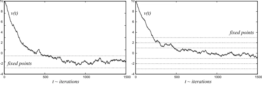
Consider a one dimensional stochastic process characterized by the iteration
vt+1= (1−γt)vt+γt(Kt(vt) +wt), (7)
whereγt is the learning rate and wt is a noise term. Let us suppose we have n alternating operators
kiwith Lipschitz constants bi<1 and fixed points v∗i where i∈ {0, . . . ,n−1},
ki(v) =v+ (1−bi)(v∗i −v).
The current operator at time t is Kt =ki(thus, Vt∗=v∗i andβt =bi) if i≡t(mod n), that is, if i is
congruent with t modulo n: if they have the same remainder when they are divided by n. In other words, we apply a round-robin type schedule for the operators.
Figure 1 shows that the trajectories remained close to the fixed points. The figure illustrates the case of two (−1 and 1) and six (−3,−2,−1,1,2,3) alternating fixed points.
0 500 1000 1500
-4 -2 0 2 4 6 8 10
t ~ iterations t ~iterations
v(t) v(t)
fixed points
fixed points
-4 -2 0 2 4 6 8 10
0 500 1000 1500
Figure 1: Trajectories generated by (7) with two (left) and six (right) fixed points.
5.2.2 A PATHOLOGICALEXAMPLE
During this example we will restrict ourselves to deterministic functions. According to the Banach
fixed point theorem, if we have a contraction mapping f over a complete metric space with fixed
point v∗= f(v∗), then, for any initial v0 the sequence vt+1= f(vt) converges to v∗. It could be
thought that this result can be easily generalized to the case of alternating operators. For example, suppose we have n alternating contraction mappings ki with Lipschitz constants bi <1 and fixed
points v∗i, respectively, where i∈ {0, . . . ,n−1}, and we apply them iteratively starting from an arbitrary v0, viz., vt+1=Kt(vt), where Kt =ki if i≡t(mod n). One may think that since each ki
attracts the point towards its fixed point, the sequence vt converges to the convex hull of the fixed
points. However, as the following example demonstrates, this is not the case, since it is possible that the point moves away from the convex hull and, in fact, it gets farther and farther after each iteration.
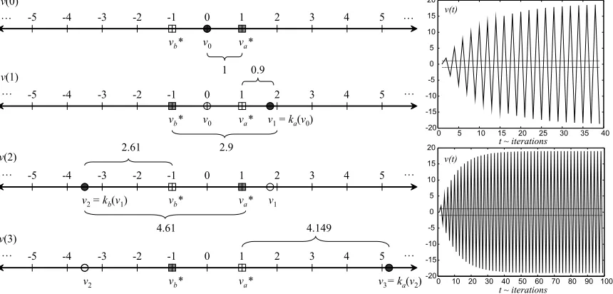
Now, let us consider two one-dimensional functions, ki:R→R, where i∈ {a,b}, defined below
and Lipschitz constants bi(in Figure 2, v∗a=1, vb∗=−1 and bi=0.9).
ki(v) =
v+ (1−bi)(v∗i −v) if sgn(v∗i) =sgn(v−v∗i),
v∗i + (v∗i −v) + (1−bi)(v−v∗i) otherwise,
(8)
where sgn(·)denotes the signum1 function. Figure 2 demonstrates that even if the iteration starts
from the middle of the convex hull (from the center of mass), v0=0, it starts getting farther and
farther from the fixed points in each step when we apply kaand kbafter each other. Nevertheless,
0 1 2 3 4 5 …
-1 -2 -3 -4 -5 … v
b* v0 va*
0 1 2 3 4 5
-1 -2 -3 -4 -5 … … v
1= ka(v0)
0 1 2 3 4 5
-1 -2 -3 -4 -5 … … v
2= kb(v1)
1
v
b* v0 va*
0.9
2.9 2.61
v
1
0 1 2 3 4 5
-1 -2 -3 -4 -5 … … v 2 4.61 v
3= ka(v2)
v
b* va*
v
b* va*
4.149 v(0)
v(1)
v(2)
v(3)
t ~ iterations
t~iterations
0 5 10 15 20 25 30 35 40 -20 -15 -10 -5 0 5 10 15 20
0 10 20 30 40 50 60 70 80 90 100 -20 -15 -10 -5 0 5 10 15 20 v(t) v(t)
Figure 2: A deterministic pathological example, generated by the iterative application of (8). The left part demonstrates the first steps, while the two images on the right-hand side show the behavior of the trajectory in the long run.
the following argument shows that sequence vt cannot get arbitrarily far from the fixed points.
Let us denote the diameter of the convex hull of the fixed points by ρ. Since this convex hull is a polygon (where the vertices are fixed points) ρ=maxi,jkvi∗−v∗jk. Furthermore, letβ0 be
defined asβ0=maxibiand dt as dt=minikv∗i −vtk. Then, it can be proven that for all t, we have
dt+1≤β0(2ρ+dt). If we assume that dt+1≥dt, then it follows that dt≤dt+1≤β0(2ρ+dt). After
rearrangement, we get the following inequality
dt≤
2β0ρ
1−β0
=φ(β0,ρ).
Therefore, dt >φ(β0,ρ) implies that dt+1 <dt. Consequently, if vt somehow got farther than φ(β0,ρ), in the next step it would inevitably be attracted towards the fixed points. It is easy to
see that this argument is valid in an arbitrary normed space, as well.
5.3 Reinforcement Learning in(ε,δ)-MDPs
In case of finite(ε,δ)-MDPs we can formulate a relaxed convergence theorem for value function based reinforcement learning algorithms, as a corollary of Theorem 20. Suppose that
V
consists of state-value functions, namely,X
=X. Then, we havelim sup
t→∞
kJ∗−Jt∗k∞≤d(ε,δ),
where Jt∗ is the optimal value function of the MDP at time t and J∗ is the optimal value function of the base MDP. In order to calculate d(ε,δ), Theorems 11 (or 10), 12 and the triangle inequality could be applied. Assume, for example, that we use the supremum norm, k·k∞, for cost functions andk·k1, defined by Equation (5), for transition functions. Then,
d(ε,δ) = εαkgk∞ (1−α)2+
δ 1−α,
where g is the cost function of the base MDP. Now, by applying Theorem 20, we have
Corollary 21 Suppose that we have an (ε,δ)-MDP and Assumptions 1-3 hold. Let Vt be the
se-quence generated by iteration (6). Furthermore, assume that the fixed point of each operator Kt is
Jt∗. Then, for any initial V0∈
V
, the sequence Vt κ-approximates J∗withκ= 4 d(ε,δ)
1−β0 .
Notice that as parametersεandδgo to zero, we get back to a classical convergence theorem for this kind of stochastic iterative algorithm (still in a little bit generalized form, sinceβt might still
change over time). Now, with the help of these results, we will investigate the convergence of some classical reinforcement learning algorithms in(ε,δ)-MDPs.
5.3.1 ASYNCHRONOUSVALUEITERATION IN(ε,δ)-MDPS
The method of value iteration is one of the simplest reinforcement learning algorithms. In ordinary MDPs it is defined by the iteration Jt+1=T Jt, where T is the Bellman operator. It is known that the
sequence Jtconverges in the supremum norm to J∗for any initial J0(Bertsekas and Tsitsiklis, 1996).
The asynchronous variant of value iteration arises when the states are updated asynchronously, for example, only one state in each iteration. In the case of (ε,δ)-MDPs a small stepsize variant of asynchronous value iteration can be defined as
Jt+1(x) = (1−γt(x))Jt(x) +γt(x)(TtJt)(x),
where Tt is the Bellman operator of the current MDP at time t. Since there is no noise term in
the iteration, Assumption 1 is trivially satisfied. Assumption 3 follows from the fact that each
Tt operator is anα contraction where α is the discount factor. Therefore, if the stepsizes satisfy
Assumption 2 then, by applying Corollary 21, we have that the sequence Jt κ-approximates J∗for
5.3.2 Q-LEARNING IN(ε,δ)-MDPS
Watkins’ Q-learning is a very popular off-policy model-free reinforcement learning algorithm (Even-Dar and Mansour, 2003). Its generalized version inε-MDPs was studied by Szita et al. (2002). The Q-learning algorithm works with action-value functions, therefore,
X
=X×A, and the one-stepQ-learning rule in(ε,δ)-MDPs can be defined as follows
Qt+1(x,a) = (1−γt(x,a))Qt(x,a) +γt(x,a)(TetQt)(x,a), (9)
(TetQt)(x,a) =gt(x,a) +α min
B∈A(Y)Qt(Y,B),
where gt is the immediate-cost function of the current MDP at time t and Y is a random variable
generated from the pair(x,a)by simulation, that is, according to the probability distribution pt(x,a),
where pt is the transition function of the current MDP at time t.
Operator Tet is randomized, but as it was shown by Bertsekas and Tsitsiklis (1996) in their
convergence theorem for Q-learning, it can be rewritten in a form as follows
(TetQ)(x,a) = (KetQ)(x,a) +Wft(x,a),
whereWft(x,a)is a noise term with zero mean and finite variance, andKet is defined as
(KetQ)(x,a) =gt(x,a) +α
∑
y∈Xpt(y|x,a) min
b∈A(y)Q(y,b).
Let us denote the optimal action-value function of the current MDP at time t and the base MDP by
Q∗t and Q∗, respectively. By using the fact that J∗(x) =minaQ∗(x,a), it is easy to see that for all
t, Q∗t is the fixed point of operatorKet and, moreover, eachKet is anαcontraction. Therefore, if the
stepsizes satisfy Assumption 2, then the Qt sequence generated by iteration (9)κ-approximates Q∗
for any initial Q0withκ= (4 d(ε,δ))/(1−α).
In some situations the immediate costs are randomized, however, even in this case the relaxed convergence of Q-learning would follow as long as the random immediate costs had finite expected value and variance, which is required for satisfying Assumption 1.
5.3.3 TEMPORALDIFFERENCELEARNING IN(ε,δ)-MDPS
Temporal difference learning, or for short TD-learning, is a policy evaluation algorithm. It aims at finding the corresponding value function Jπfor a given control policyπ(Bertsekas and Tsitsiklis, 1996; Sutton and Barto, 1998). It can also be used for approximating the optimal value function, for example, if we apply it together with the policy iteration algorithm.
First, we briefly review the off-line first-visit variant of TD(λ) in case of ordinary MDPs. It can be shown that the value function of a policyπcan be rewritten in a form as
Jπ(x) =E
" ∞
∑
m=0
(αλ)mDπ α,m
X0=x
#
+Jπ(x),
whereλ∈[0,1)and Dπα,mdenotes the “temporal difference” coefficient at time m,
where Xm, Xm+1and Aπmare random variables, Xm+1has p(Xm,Aπm)distribution and Aπmis a random
variable for actions, it is selected according to the distributionπ(Xm).
Based on this observation, we can define a stochastic approximation algorithm as follows. Let us suppose that we have a generative model of the environment, for example, we can perform simulations in it. Each simulation produces a state-action-reward trajectory. We can assume that all simulations eventually end, for example, there is an absorbing termination state or we can stop the simulation after a given number of steps. Note that even in this case we can treat each trajectory as infinitely long, viz., we can define all costs after the termination as zero. The off-line first-visit TD(λ) algorithm updates the value function after each simulation,
Jt+1(xtk) =Jt(xtk) +γt(xtk) ∞
∑
m=k
(αλ)m−kdα,m,t, (10)
where xtk is the state at step k in trajectory t and dα,m,t is the temporal difference coefficient,
dα,m,t =g(xtm,atm) +αJt(xtm+1)−Jt(xtm).
For the case of ordinary MDPs it is known that TD(λ) converges almost surely to Jπ for any initial J0provided that each state is visited by infinitely many trajectories and the stepsizes satisfy
Assumption 2. The proof is based on the observation that iteration (10) can be seen as a Robbins-Monro type stochastic iterative algorithm for finding the fixed point of Jπ=HJπ, where H is a contraction mapping with Lipschitz constantα(Bertsekas and Tsitsiklis, 1996). The only difference in the case of(ε,δ)-MDPs is that the environment may change over time and, therefore, operator
H becomes time-dependent. However, each Ht is still anα contraction, but they potentially have
different fixed points. Therefore, we can apply Theorem 20 to achieve a relaxed convergence result for off-line first-visit TD(λ) in changing environments under the same conditions as in the case of ordinary MDPs.
The convergence of the on-line every-visit variant can be proven in the same way as in the case of ordinary MDPs, viz., by showing that the difference between the two variants is of second order in the size ofγt and hence inconsequential asγt diminishes to zero.
5.3.4 APPROXIMATEDYNAMICPROGRAMMING
Most RL algorithms in their standard forms, for example, with lookup table representations, are highly intractable in practice. This phenomenon, which was named “curse of dimensionality” by Bellman, has motivated approximate approaches that result in more tractable methods, but often yield suboptimal solutions. These techniques are usually referred to as approximate dynamic
pro-gramming (ADP). Many ADP methods are combined with simulation, but their key issue is to
approximate the value function with a suitable approximation architecture: V ≈Φ(r), where r is a parameter vector. Direct ADP methods collect samples by using simulation, and fit the architecture to the samples. Indirect methods obtain parameter r by using an approximate version of the Bellman equation (Bertsekas, 2007).
The power of the approximation architecture is the smallest error that can be achieved, η=
infrkV∗−Φ(r)k, where V∗ is the optimal value function. Suppose thatη>0, then no algorithm
In general, many direct and indirect ADP methods can be formulated as follows
Φ(rt+1) =Π (1−γt)Φ(rt) +γt(Bt(Φ(rt)) +Wt)
, (11)
where rt ∈Θ is an approximation parameter, Θ is the parameter space, for example, Θ⊆Rp, Φ:Θ→
F
is an approximation architecture whereF
⊆V
is a Hilbert space that can be repre-sented by usingΦwith parameters fromΘ. FunctionΠ:V
→F
is a projection mapping, it renders a representation fromF
to each value function fromV
. Operator Bt :F
→V
acts on(approxi-mated) value functions. Finally,γt denotes the stepsize and Wt is a noise parameter representing the
uncertainties coming from, for example, the simulation.
Operator Bt is time-dependent since, for example, if we model an approximate version of
opti-mistic policy iteration, then in each iteration the control policy changes and, therefore, the update operator changes, as well. We can notice that ifΠwas a linear operator (see below), Equation (11) would be a stochastic iterative algorithm with Kt=ΠBt. Consequently, the algorithm described by
Equation (6) is a generalization of many ADP methods, as well.
Now, we show that a convergence theorem for ADP methods can also be deduced by using Theorem 20. In order to apply the theorem, we should ensure that each update operator be a con-traction. If we assume that every Bt is a contraction, we should require two properties fromΠto
guarantee that the resulted operators remain contractions. First,Πshould be linear. OperatorΠis linear if it is additive and homogeneous, more precisely, if∀V1,V2:Π(V1+V2) =Π(V1) +Π(V2)
and ∀V :∀α:Π(αV) =αΠ(V), where α is a scalar. This requirement allows the separation of the components. Moreover, Π should be nonexpansive w.r.t. the supremum norm, namely:
∀V1,V2:kΠ(V1)−Π(V2)k ≤ kV1−V2k. Then, the update operator of the algorithm, Kt =ΠBt,
is guaranteed to be a contraction.
If we assume that Vt∗is the fixed point of Kt, thus,(ΠBt)Vt∗=Vt∗andβt is the Lipschitz constant
of Kt with lim supt→∞βt =β0<1, we can deduce a convergence theorem for ADP methods, as a
corollary of Theorem 20. Suppose that Assumptions 1-2 hold and each Bt is a contraction as well
asΠis linear and supremum norm nonexpansive, thenΦ(rt)κ-approximates V∗for any initial r0
with κ=4ρ/(1−β0), where ρ=lim supt→∞kVt∗−V∗k. In case all of the fixed points were the
same, viz.,∀t : V0∗=Vt∗, thenΦ(rt)would converge to V0∗almost surely, consequently,Φ(rt)would κ-approximate V∗withκ=kV0∗−V∗k.
Naturally, these results are quite loose, since we did not make strong assumptions on the applied algorithm and on the approximation architecture. They only illustrate that the approach we took, which allows time-dependent update operators and analyzes approximate convergence, could also provide results for ordinary MDPs, for example, in the case of ADP.
6. Experimental Results
In this section we present two numerical experiments. The first one demonstrates the effects of environmental changes during Q-learning based scheduling. The second one presents a parameter analysis concerning the effectiveness of SARSA in(ε,δ)-type grid world domains.
6.1 Environmental Changes During Scheduling
job-shop scheduling problem (JSP) is one of the basic scheduling problems (Pinedo, 2002). We
investigated an extension of JSP, called the flexible job-shop scheduling problem (FJSP), in which some of the resources are interchangeable, that is, there may be tasks that can be executed on several resources. This problem can be formulated as a finite horizon MDP and can be solved by Q-learning based methods (Cs´aji and Monostori, 2006).
170 190 210 230 250 270 290 310 330
1 20 40 60 80 100 120 140 160 180 170
190 210 230 250 270 290 310 330
1 20 40 60 80 100 120 140 160 180 200 200
t ~time t ~time
k(t) k(t)
(a) (b)
k’(t)
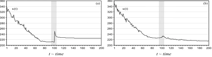
Figure 3: The black curves,κ(t), show the performance measure in case there was a resource break-down (a) or a new resource availability (b) at time t=100; the gray curve in (a),κ’(t), demonstrates the case the policy would be recomputed from scratch.
200 220 240 260 280 300 320 340 360
1 20 40 60 80 100 120 140
60 80 100 120 140 160 180 200
k(t)
(a) (b)
t ~time t ~time
160 180
200 220 240 260 280 300 320 340 360
1 20 40 200
k(t)
Figure 4: The black curves,κ(t), show the performance measure during resource control in case there was a new job arrival (a) or a job cancellation (b) at time t=100.
Recall that Theorems 10, 11 and 12 measure the amount of the possible change in the value function in case there were changes in the MDP, but since these theorems apply supremum norm, they only provide bounds for worst case situations. However, the results of our numerical exper-iments, shown in Figures 3 and 4, are indicative of the phenomenon that in an average case the change is much less. Therefore, applying the obsolete value function after a change took place is preferable over restarting the optimization from scratch.
The results, black curves, show the case when the obsolete value function approximation was applied after the change took place. The performance which would arise if the system recomputed the whole schedule from scratch is drawn in gray in part (a) of Figure 3.
6.2 Varying Grid World
We also performed numerical experiments on a variant of the classical grid world problem (Sutton and Barto, 1998). The original version of this problem can be briefly described as follows: an agent wanders in a rectangular world starting from a random initial state with the aim of finding the goal state. In each state the agent is allowed to choose from four possible actions: “north”, “south”, “east” and “west”. After an action was selected, the agent moves one step in that direction. There are some mines on the field, as well, that the agent should avoid. An episode ends if the agent finds the goal state or hits a mine. During our experiments, we applied randomly generated 10×10 grid worlds (thus, these MDPs had 100 states) with 10 mines. The immediate-cost of taking a (non-terminating) step was 5, a cost of hitting a mine was 100 and the cost of finding the goal state was
−100.
In order to perform the experiment described by Table 1, we have applied the “RL-Glue” frame-work2 which consists of open source softwares and aims at being a standard protocol for bench-marking and interconnecting reinforcement learning agents and environments.
We have analyzed an (ε,δ)-type version of grid world, where the problem formed an (ε,δ) -MDP. More precisely, we have investigated the case when for all time t, the transition-probabilities could vary by at mostε≥0 around the base transition-probability values and the immediate-costs could vary by at mostδ≥0 around the base cost values.
During our numerical experiments, the environment changed at each time-step. These changes were generated as follows. First, changes concerning the transition-probabilities are described. In our randomized grid worlds the agent was taken to a random surrounding state (no matter what action it chose) with probabilityη and this probability changed after each step. The newη was computed according to the uniform distribution, but its possible values were bounded by the values described in the first row of Table 1.
Similarly, the immediate-costs of the base MDP (cf. the first paragraph) were perturbed with a uniform random variable that changed at each time-step. Again, its (absolute) value was bounded byδ, which is presented in the first column of the table. The values shown were divided by 100 to achieve the same scale as the transition-probabilities have.
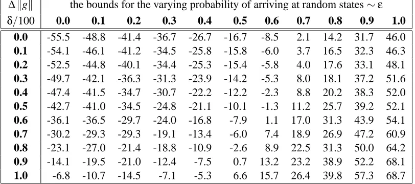
Table 1 was generated using an (optimistic) SARSA algorithm, namely, the current policy was evaluated by SARSA, then the policy was (optimistically) improved, more precisely, the greedy policy with respect to the achieved evaluation was calculated. That policy was also soft, namely, it made random explorations with probability 0.05. We have generated 1000 random grid worlds for each parameter pairs and performed 10 000 episodes in each of these generated worlds. The results
∆kgk the bounds for the varying probability of arriving at random states∼ε
δ/100 0.0 0.1 0.2 0.3 0.4 0.5 0.6 0.7 0.8 0.9 1.0
0.0 -55.5 -48.8 -41.4 -36.7 -26.7 -16.7 -8.5 2.1 14.2 31.7 46.0
0.1 -54.1 -46.1 -41.2 -34.5 -25.8 -15.8 -6.0 3.7 16.5 32.3 46.3
0.2 -52.5 -44.8 -40.1 -34.4 -25.3 -15.4 -5.8 4.0 17.6 33.1 48.1
0.3 -49.7 -42.1 -36.3 -31.3 -23.9 -14.2 -5.3 8.0 18.1 37.2 51.6
0.4 -47.4 -41.5 -34.7 -30.7 -22.2 -12.2 -2.3 8.8 20.2 38.3 52.0
0.5 -42.7 -41.0 -34.5 -24.8 -21.1 -10.1 -1.3 11.2 25.7 39.2 52.1
0.6 -36.1 -36.5 -29.7 -24.0 -16.8 -7.9 1.1 17.0 31.3 43.9 54.1
0.7 -30.2 -29.3 -29.3 -19.1 -13.4 -6.0 7.4 18.9 26.9 47.2 60.9
0.8 -23.1 -27.0 -21.4 -18.8 -10.9 -2.6 8.9 22.5 31.3 50.0 64.2
0.9 -14.1 -19.5 -21.0 -12.4 -7.5 0.7 13.2 23.2 38.9 52.2 68.1
1.0 -6.8 -10.7 -14.5 -7.1 -5.3 6.6 15.7 26.4 39.8 57.3 68.7
Table 1: The (average) cumulative costs gathered by SARSA in varying grid worlds.
presented in the table were calculated by averaging the cumulative costs over all episodes and over all generated sample worlds.
The parameter analysis shown in Table 1 is indicative of the phenomenon that changes in the transition-probabilities have a much higher impact on the performance. Even large perturbations in the costs were tolerated by SARSA, but large variations in the transition-probabilities caused a high decrease in the performance. An explanation could be that large changes in the transitions cause the agent to loose control over the events, since it becomes very hard to predict the effects of the actions and, hence, to estimate the expected costs.
7. Conclusion
The theory of MDPs provide a general framework for modeling decision making in stochastic dy-namic systems, if we know a function that describes the dydy-namics or we can simulate it, for example, with a suitable program. In some situations, however, the dynamics of the system may change, too. In theory, this change can be modeled with another (higher level) MDP, as well, but doing so would lead to models which are practically intractable.
In the paper we have argued that the optimal value function of a (discounted) MDP Lipschitz continuously depends on the transition-probability function and the immediate-cost function, there-fore, small changes in the environment result only in small changes in the optimal value function. This result was already known for the case of transition-probabilities, but we have presented an improved estimation for this case, as well. A bound for changes in the discount factor was also proven, and it was demonstrated that, in general, this dependence was not Lipschitz continuous. Additionally, it was shown that changes in the discount rate could be traced back to changes in the immediate-cost function. The application of the Lipschitz property helps the theoretical treatment of changing environments or inaccurate models, for example, if the transition-probabilities or the costs are estimated statistically, only.