Deterministic Error Analysis of Support Vector Regression and Related Regularized Kernel Methods

Deterministic Error Analysis of Support Vector Regression and

Related Regularized Kernel Methods

Christian Rieger [email protected]

Institute for Numerical Simulation & Hausdorff Center for Mathematics University of Bonn

Wegelerstr. 6, 53115 Bonn, Germany

Barbara Zwicknagl [email protected] Institute for Applied Mathematics & Hausdorff Center for Mathematics

University of Bonn

Endenicher Allee 60, 53115 Bonn, Germany

Editor: Bernhard Schölkopf

Abstract

We introduce a new technique for the analysis of kernel-based regression problems. The basic tools are sampling inequalities which apply to all machine learning problems involving penalty terms induced by kernels related to Sobolev spaces. They lead to explicit deterministic results concerning the worst case behaviour ofε- andν-SVRs. Using these, we show how to adjust regularization parameters to get best possible approximation orders for regression. The results are illustrated by some numerical examples.

Keywords: sampling inequality, radial basis functions, approximation theory, reproducing kernel

Hilbert space, Sobolev space

1. Introduction

Support Vector (SV) machines and related kernel-based algorithms are modern learning systems motivated by results of statistical learning theory as introduced by Vapnik (1995). The concept of SV machines is to provide a prediction function which is accurate on the given training data and which is sparse in the sense that it can be written in terms of a typically small subset of all sam-ples, called the support vectors, as stated by Schölkopf et al. (1995). Therefore, SV regression and classification algorithms are closely related to regularized problems from classical approximation theory as pointed out by Girosi (1998) and Evgeniou et al. (2000) who had applied techniques from functional analysis to derive probabilistic error bounds for SV regression.

This paper provides a theoretical framework to derive deterministic error bounds for some popular SV machines. We show how a sampling inequality by Wendland and Rieger (2005) can be used to bound the worst-case generalization error for theν- and theε-regression without making any statistical assumptions on the inaccuracy of the training data. In contrast to the literature, our error bounds explicitly depend on the pointwise noise in the data. Thus they can be used for any subse-quent probabilistic analysis modelling certain assumptions on the noise distribution.

al-gorithms. We provide a deterministic error analysis for theν- and theε-SVR for both exact and inexact training data. Our analytical results showing optimal convergence orders in Sobolev spaces are illustrated by numerical experiments.

2. Reproducing Kernels in Hilbert Spaces

We suppose that K is a positive definite kernel on some domainΩ_⊂Rd _{which should contain at} least one point. To start with, we briefly recall the well known definition of a reproducing kernel in a Hilbert space. In the following we shall use the notation that bold letters denote vectors, that is

v= (v1, . . . ,vd)T ∈Rd.

Definition 1 Let

H

(Ω) be a Hilbert space of functions f :Ω_→R_{. A function K :}Ω_×Ω_→R_is

called reproducing kernel of

H

(Ω), if

• K(y,_·)_∈

H

(Ω)for all y_∈Ω and

• f(y) = (f,K(y,_·))H(Ω)for all f ∈

H

(Ω)and all y∈Ω.

For each positive definite kernel K :Ω_×Ω_→R_{there exists a unique Hilbert space}

N

_K(Ω)of func-tions f :Ω→R_{, such that K is the reproducing kernel of}

N

_K(Ω)(see Wendland, 2005, Theorems 10.1 and 10.11). This Hilbert space

N

K(Ω)is called the native space of K. Though this definition

of a native space is rather abstract, it can be shown that in some cases the native spaces coincide with classical function spaces.

From now on we shall only consider radial kernels K, that is,

K(x,y) =K(_kx₋y_k) for all x,y_∈Rd _,

where we use the same notation for the kernel K :Rd_×Rd _→R_{and for the function K :}Rd_→R_. We hope that this does not cause any confusion. We shall mainly focus on continuous kernels

K∈L1(Ω), that is,

kKkL1(Ω):=

Z

Ω|K(x)|dx<∞.

For K_∈L1 Rd_{, we define the Fourier transform ˆK by}

ˆ

K(ω) := (2π)−d2

Z

RdK(x)e

−ix·ω_{dx, ω∈R}d_.

For the caseΩ=Rd_{there is the following characterization of native spaces of certain radial kernels}

K :Ω_→Rd_{(Wendland, 2005, Theorem 10.12).}

Theorem 2 Suppose that K∈C(Rd_)∩L1(Rd_{)is a real-valued and positive definite radial kernel.} Then the native space of K is given by

N

_K(Rd) =

f ∈L2(Rd)_∩C(Rd) : √fˆ

ˆ

K ∈L2(

Rd)

,

(f,g)NK(Rd) = (2π)

−d/2 _ˆ

f √

ˆ

K,

ˆ

g √

ˆ

K

L2(Rd) ,

We recall that the Sobolev spaces W₂s(Rd)onRd _{with s≥0 are given by}

W₂s(Rd_):=n_{f ∈L2(}Rd_{) : ˆf(·)(1+k·k}2

2)s/2∈L2(Rd) o

. (1)

Therefore for a radial kernel function K whose Fourier transform decays like

c1(1+_k·k2₂)s_{≤Kˆ ≤c2(1+k·k}2

2)s ,s>d/2 (2)

for some constants c1,c2>0, the associated native space

N

K(Rd) is W2s(Rd) with an equivalent

norm. There are several examples of kernels satisfying the condition (2). One famous example for fixed s_∈(d/2,∞)is the Matern kernel (Wendland, 2005)

Ks(x):=

21−s

Γ(s)kxk

s−d/2

2

K

d/2−s(kxk2),

where

K

denotes the Bessel function of the third kind. In our examples, however, we focus on

Wendland’s functions (Wendland, 2005). They are very convenient to implement since they are

compactly supported and piecewise polynomials. Such nice reproducing kernels are so far only available for certain choices of the space dimension d and the decay parameter s (see Wendland, 2005), but a recent result by Schaback (2009) covers almost all cases of practical interest. We shall explain some more properties of these kernels in the experimental part, see Section 10, and refer to the recent monograph by Wendland (2005) for details.

In order to establish the equivalence of native spaces and Sobolev spaces on bounded domains one needs certain extension theorems for Sobolev functions on bounded domains (see Wendland, 2005).

Definition 3 LetΩ_⊂Rd_{be a domain. We define the Sobolev spaces of integer orders k∈}N_as

W₂k(Ω) =_{f _∈L2(Ω) : f has weak derivatives Dαf _∈L2(Ω)of order_|α_{| ≤}k_} with the norm

ku_kWk

2(Ω):=

∑

|α|≤k

kDαu_k2_L

2(Ω)

!1/2

.

For fractional smoothness s=k+σwith 0<σ<1 and k_∈N_{we define the semi-norm}

|u_|Ws

2(Ω):=

∑

|α|=k

Z

Ω Z

Ω

|Dαu(x)₋Dαu(y)|2 kx₋y_kd₂+2σ dxdy

!1/2

,

and set

W₂s(Ω):=

u∈L2(Ω) :

kukW2k

2(Ω)+|u|

2 Ws

2(Ω)

1/2

<∞

.

In the caseΩ=Rd _{this space is known to be equivalent to the space given by (1) in terms of Fourier}

Theorem 4 Suppose that K∈L1(Rd)has a Fourier transform that decays as(1+_k·k2₂)−s_{for s>}

d/2. Suppose thatΩhas a Lipschitz boundary. Then

N

_K(Ω)∼=W₂s(Ω)

with equivalent norms.

3. Regularized Problems in Native Hilbert Spaces

In the native Hilbert spaces we consider the following learning or recovery problem. We assume that we are given (possibly only approximate) function values y1, . . . ,yN ∈Rof an unknown function

f_∈

N

_K(Ω)on some scattered points X :=

x(1)_{, . . . ,x}(N) _{⊂Ω, that is f x}(j)

≈yjfor j=1, . . . ,N.

In the following we shall use the notation that bold letters denote vectors, that is v= (v1, . . . ,vd)T∈

Rd_.

To control accuracy and complexity of the reconstruction simultaneously, we use the optimization problem

min

s∈NK(Ω) ε∈R+

1

N N

∑

j=1 V_ε

s

x(j)

−yj

+ 1

2Cksk

2

NK(Ω) , (3)

where C>0 is a positive parameter and V_εdenotes a positive function which may be parametrized by a positive real numberε. We point out that Vε need not be a classical loss function. Therefore we shall give some proofs of results which were formulated by Schölkopf and Smola (2002) in the case of V_εbeing a loss function.

Theorem 5 (Representer theorem) If(sX,y,ε∗)is a solution of the optimization problem (3), then there exists a vector w_∈RN _{such that}

sX,y(·) = N

∑

j=1 wjK

x(j),_·,

that is sX,y∈span

K x(1),_·

, . . . ,K x(N),_· .

Proof For the readers’ convenience, we repeat the proof from Schölkopf and Smola (2002) in our

specific situation. Every s_∈

N

K(Ω) can be decomposed into two parts s=s_||+s_⊥, where s_|| is

contained in the linear span of

K x(1)_,·

, . . . ,K x(N)_{,· , and s}

⊥ is contained in the orthogonal complement, that iss_||,s_⊥N

K(Ω)=0. By the reproducing property of the kernel K in the native

space, the problem (3) can be rewritten as

min

s=s_||+s⊥ ε∈R+

1

N N

∑

j=1 V_ε

D

s_||,K

x(j),_·E₋yj

+ 1

2C

s_||

2 NK(Ω)+

1 2Cks⊥k

2 NK(Ω) .

Therefore a solution(sX,y,ε∗)of the optimization problem (3) satisfies(sX,y)_⊥=0, which implies sX,y∈span

K x(1),_·

, . . . ,K x(N),_· .

Corollary 6 If sX,yis a solution of the optimization problem

min

s∈NK(Ω)

1

N N

∑

j=1 Vε

s

x(j)

−yj

+ 1

2Cksk

2

NK(Ω) , (4)

withε_∈R+ _{being a fixed parameter, then sX,y∈spanK x}(1)_{,·, . . . ,K x}(N)_{,· .}

The representer theorems can be used to reformulate infinite-dimensional optimization problems of the forms (3) or (4) in a finite-dimensional setting (see Schölkopf and Smola, 2002).

4. Support Vector Regression

As a first optimization problem of the form (3) we consider theν-SVR which was introduced by Schölkopf et al. (2000). The function Vε(x) =_|x_|ε+ενis related to Vapnik’sε-intensive loss func-tion (Vapnik, 1995)

|x|ε=

0 i f_|x_{| ≤}ε |x_{| −}ε i f_|x_|>ε ,

but has an additional term with a positive parameter ν. The associated optimization problem is calledν-SVR and takes the form

min

s∈NK(Ω) ε∈R+

1

N N

∑

j=1 s

x(j)

−yj

_ε+εν+

1 2Cksk

2

NK(Ω) . (5)

Theorem 7 The optimization problem (5) possesses a solutions(_Xν_,)_y,ε∗_.

Proof This follows from a general result by Micchelli and Pontil (2005). The problem (5) is

equivalent to the optimization problem

min

s_∈NK(Ω) δ∈R

1

N N

∑

j=1 s

x(j)

−yj

_δ2+δ

2_ν+ 1

2Cksk

2

NK(Ω) . (6)

If we set

H

:=

N

_K(Ω)_×R_{we can define an inner product on}

H

by

hh1,h2iH :=hf1,f2iNK(Ω)+2Cνhr1,r2iR

for hj = (fj,rj), j=1,2. To make

H

a space of functions we use the canonical identification of

R _{with the space of constant functions}R_→R_{. The Hilbert space}

H

then has the reproducing kernel ˜K := K, 1

2Cν1

where 1 denotes the constant function which maps everything to 1, that is ˜

K((x,r),(y,s)) =K(x,y) +1/(2Cν) for all r,s_∈R_{. With this notation the problem (6) can be} rewritten as

min

(s,δ)∈HQ y_(I

X(s,δ)) +

1

2Ck(s,δ)k

2

H , (7)

where

IX(s,δ):=

and

Qy:RN+1_→R_{, Q}y_(p,δ_{) =} 1

N N

∑

j=1 p_j−y_j

_δ2.

Since Qyis continuous onRN+1_{for all y∈}RN_{, the problem (7) possesses a solution as shown by} Micchelli and Pontil (2005).

If we introduce the slack variablesξ,ξ∗_∈RN_{, the representer theorem gives us an equivalent} finite-dimensional problem which was considered by Schölkopf et al. (2000).

min

w∈RN

ξ∗_,ξ∈RN ε∈R+

1 2w

T_{Kw+C νε+}1 N

N

∑

j=1

ξj+ξ∗j

!

subject to (Kw)_j−yj ≤ ε+ξj,

(₋Kw)_j+yj ≤ ε+ξ∗j ,

ξ∗

j,ξj≥0, ε≥0 for 1≤ j≤N, (8)

where

K=K

x(i),x(j)

i,j=1...N

denotes the Gram matrix of the kernel K. We will use this equivalent problem for implementation and our numerical tests.

A particularly interesting problem arises if we skip the parameter νand let εbe fixed. Then the optimization problem (8) takes the form

min

w∈RN

ξ∗_,ξ∈RN

1 2w

T_Kw+C1 N

N

∑

j=1

ξj+ξ∗j

subject to (Kw)_j−yj ≤ ε+ξj,

(₋Kw)_j+yj ≤ ε+ξ∗j ,

ξ∗

j,ξj ≥ 0 for 1≤ j≤N. (9)

Schölkopf et al. (2000) called this problem ε-SVR. Similarly to theν-SVR, the problem (9) can be formulated as a regularized minimization problem in a Hilbert space (Evgeniou et al., 2000), namely

min

s_∈NK(Ω)

1

N N

∑

j=1 s

x(j)

−yj

_ε+

1 2Cksk

2

NK(Ω) . (10)

Like the ν-SVR, this optimization problem possesses a solution (see Micchelli and Pontil, 2005, Lemma 1).

5. A Sampling Inequality

domain with Lipschitz boundary that satisfies an interior cone condition. A domain Ωis said to satisfy an interior cone condition with radius r>0 and angleθ_∈ 0,π₂

if for every x_∈Ωthere is a unit vectorξ(x)such that the cone

C(x,ξ(x),θ,r):=nx+λy : y_∈Rd_,kyk2=1,yTξ_(x)≥cos(θ_),λ_∈[0,r]

o

is contained inΩ. In particular, a domain which satisfies an interior cone condition cannot have any outward cusps. We shall assume for the rest of this paper thatΩsatisfies an interior cone condition with radius Rmaxand angleθ. We shall derive estimates that are valid only if the training points are

sufficiently dense inΩ. To make this condition precise, we will need a slightly unhandy constant which depends only on the geometry ofΩ, namely (see Wendland, 2005)

CΩ:=

sin

2 arcsin

sinθ 4(1+sinθ)

sinθ

8

1+sin

2 arcsin

sinθ 4(1+sinθ)

(1+sinθ)

Rmax.

Suppose that K is a radial kernel function such that the native Hilbert space of K is norm-equivalent to a Sobolev space, that is

N

_K(Ω) =W₂τ(Ω). Here we assume that⌊τ−1

2⌋>d/2, where we use the

notation⌊t⌋:=max{n∈N_{0: n≤t}for t≥0. Furthermore, let X}=

x(1), . . . ,x(N) ⊂Ωbe a finite set with sufficiently small fill distance

h :=hX,Ω:=sup

x_∈Ω

min

x(j)_∈X x−x

(j)

2 .

The fill distance can be interpreted geometrically as the radius of the largest ball with center in ¯

Ωthat does not contain any of the points x(1), . . . ,x(N). It is a useful quantity for the deterministic error analysis in Sobolev spaces. The case h=0 implies that X=

x(1), . . . ,x(N) is dense inΩ, and therefore convergence is studied for the limit h_→0 which means that the domainΩis equally filled with points from X . Let us explain the relation to the usual error bounds in terms of the number of points N. In the case of regularly distributed points we have that h=cN−d1 with some constant

c>0 (Wendland, 2005). Therefore the limit h_→0 is equivalent to the limit N_→∞which is the more intuitive meaning of asymptotic convergence. But there is a drawback, since the error bounds in terms of N depend crucially on the space dimension d, while error bounds in terms of the fill distance h are dominated by the smoothness of the function to be learned. We will comment on this again later for the special error bounds we consider here. We shall use the following result by Wendland and Rieger (2005).

Theorem 8 SupposeΩ_⊂Rd_{is a bounded domain with Lipschitz boundary that satisfies an interior}

cone condition. Letτbe a positive real number with_⌊τ₋1_2⌋>d

2, and let 1≤q≤∞. Then there exists a positive constant C>0 such that for all discrete sets X _⊂Ωwith sufficiently small fill distance h :=hX,Ω≤CΩτ−2the inequality

ku_kL

q(Ω)≤C

hτ−d(12− 1

q)+k_uk

W₂τ(Ω)+ku|Xkℓ∞(X)

holds for all u_∈W₂τ(Ω), where we use the notation(t)+:=max{0,t}.

We shall apply this theorem to the residual function f ₋sX,y of the function f ∈W₂τ(Ω) to be

recovered and a solution sX,y∈W2τ(Ω) of the regression problem. In our applications we shall

6. ν-SVR with Exact Data

In order to derive error bounds for the ν-SVR optimization problem (5) we shall apply Theo-rem 8 to the residual f−s(_Xν_,)_y, where

s(_Xν_,)_y,ε∗ _{denotes a solution to the problem (5) for X :=}

x(1), . . . ,x(N) ⊂Ωand y∈RN_{. In this section we consider exact data, that is}

f

x(j)

=yj for j=1, . . . ,N (11)

for a function f _∈W₂τ(Ω)∼=

N

K(Ω). As pointed out by Wendland and Rieger (2005) we first need

a stability and a consistency estimate for the solution s(_Xν_,)_y.

Lemma 9 Under the assumption (11) concerning the data, we find that for every X a solution

s(_Xν_,)_y,ε∗_{to problem (5) satisfies}

s

(ν)

X,y _N

K(Ω) ≤ k

f_kN

K(Ω) and

s

(ν)

X,y|X−y

ℓ∞(X) ≤

N

2Ckfk

2

NK(Ω)+ε

∗_{·(1−Nν) .}

Proof We denote the objective function of the optimization problem (5) by

H_Cy_,ν(s,ε):= 1

N N

∑

j=1 s

x(j)

−yj

_ε+νε+

1 2Cksk

2

NK(Ω) , (12)

and the interpolant to f with respect to X and K with If, that is If|X=y and If ∈span

K x(1),_·

, . . . ,K x(N),_· . With this notation we have

1 2C

s

(ν)

X,y 2 NK(Ω)

≤H_Cy_,ν

s(_Xν_,)_y,ε∗_≤H_Cy_,ν(If,0) =

1 2C I_f 2 NK(Ω)≤

1 2Ckfk

2 NK(Ω)

sinceI_{f N}

K(Ω)≤ kfkNK(Ω)(Wendland, 2005), which implies the first claim.

Furthermore we have for i=1, . . . ,N

s

(ν)

X,y

x(i)

−yi ≤

N

∑

j=1 s

(ν)

X,y

x(j)

−yj _ε∗+ε

∗_≤NHy C,ν

s(_Xν_,)_y,ε∗+ε∗(1₋Nν)

≤ NH_Cy_,ν(If,0) +ε∗(1−Nν)≤ N 2C If 2

NK(Ω)+ε

∗_(1−Nν)

≤ N

2Ckfk

2

NK(Ω)+ε

∗_{(1−Nν) ,}

which finishes the proof.

With Theorem 8 we find immediately the following result.

Theorem 10 SupposeΩ_⊂Rd _{is a bounded domain with Lipschitz boundary that satisfies an}

inte-rior cone condition. Letτbe a positive real number with_⌊τ₋1_2⌋> d

f _∈W₂τ(Ω)with f x(i)=yi. Let

s(_Xν_,)_y,ε∗be a solution of theν-SVR. Then there is a constant

˜

C>0, which depends onτ, d andΩbut not on f or X , such that the approximation error can be bounded by

f−s

(ν)

X,y

Lq(Ω)≤

˜

C

2hτ−d( 1 2−

1

q)_+kfk

W2τ(Ω)+

N

2Ckfk

2

W2τ(Ω)+ (1−Nν)·ε ∗

for all discrete sets X _⊂Ωwith fill distance h :=hX,Ω≤CΩτ−2.

Proof Combining Lemma 9 and Theorem 8 leads to

f−s

(ν)

X,y

Lq(Ω) ≤

˜

C

hτ−d(

1 2−

1

q)₊

f−s

(ν)

X,y

W₂τ(Ω)+

y−s

(ν)

X,y|X

ℓ∞(X)

≤ C˜

hτ−(

d

2−

d q)₊

kf_kWτ

2(Ω)+

s

(ν)

X,y

W₂τ(Ω)

+

y−s

(ν)

X,y|X

ℓ∞(X)

≤ _C˜

2hτ−(d2−dq)_+kfk

W₂τ(Ω)+

N

2Ckfk

2

W₂τ(Ω)+ (1−Nν)ε∗

.

At first glance the term containing ε∗ seems to be odd because it could be uncontrollable. But according to Chang and Lin (2002) we can at least assumeε∗to be bounded by

ε∗_≤1

2

max

i=1,...,Nyi−i=min1,...,Nyi

.

If this inequality is not satisfied, the problem (8) possesses only the trivial solution s_≡0 which is not interesting. Furthermore, we see that theε∗-term occurs with a factor(1₋Nν), which can be used to control this term. If we chooseν_{≥ N}1, the term(1₋Nν)ε∗ _{vanishes or is even negative.} The parameterνis a lower bound on the fraction of support vectors (see Schölkopf et al., 2000), and henceν=1/N means to get at least one support vector, that is a non-trivial solution. Since we

are not interested in the case of trivial solutions, the conditionν_≥1/N is a reasonable assumption.

On the other hand, we can use the results from Lemma 9 to derive a more explicit upper bound on

ε∗_=ε∗_(C,ν,f)by

0_≤

s

(ν)

X,y|X−y

ℓ∞(X)≤

N

2Ckfk

2

NK(Ω)+ε

∗_{(1−Nν) .}

If we assumeν>1/N, this leads to

ε∗_=ε∗_(C,ν,f)≤ N

2C(Nν₋1)kfk

2 NK(Ω) .

We shall now make our bounds more explicit for the case of quasi-uniformly distributed points. In this case the number of points N and the fill distance h are related to each other by

c1N−1/d≤h≤c2N−1/d, (13)

where c1and c2denote positive constants (see Wendland, 2005, Proposition 14.1).

Corollary 11 In case of quasi-uniform exact data we can choose the problem parameters as

C=NkfkW2τ(Ω)

2hτ ≈h

−(τ+d)_kfk

W₂τ(Ω) andν≥

1

N to get

f−s

(ν)

X,y

L2(Ω)≤ ˜

Chτ_kf_kWτ 2(Ω)≤

˜

CN−dτk_fk

W2τ(Ω) ;

or as

C=NkfkW2τ(Ω) 2hτ−d2 ≈

h−(τ+d2)k_fk

W2τ(Ω) andν≥ 1

N to get

f−s

(ν)

X,y

L∞(Ω)≤

˜

Chτ−d2k_fk

W₂τ(Ω)≤CN˜ −

τ d+

1 2k_fk

W₂τ(Ω)

for all discrete sets X_⊂Ωwith fill distance h :=hX,Ω≤CΩτ−2, with generic positive constants ˜C

which depend onτ, d,Ωbut not on f or X .

Note that these bounds yield arbitrarily high convergence orders, provided that the functions are smooth enough, that isτ is large enough. Therefore they are in this setting better than the usual minimax rate N−2τ2+τd _{(see Stone, 1982). In the following we shall only give our error estimates in}

terms of the fill distance h rather than in terms of the number of points N. This is due to the fact that the approximation rateτin h is independent of the space dimension d. However it should be clear how the approximation rates translate into error estimates in terms of N in the case of quasi-uniform data due to the inequality (13). Note that the parameter choice in the case of arbitrary, non-uniformly distributed data can be treated analogously.

Corollary 11 shows, that the solution of the ν-SVR leads to the same approximation orders with respect to the fill distance h as classical kernel-based interpolation (see Wendland, 2005). But the

ν-SVR allows for much more flexibility and less complicated solutions. Our numerical results will confirm these convergence rates.

7. ν-SVR with Inexact Data

In this section we denote again by s(_Xν_,)_y,ε∗ _{the solution to the problem (5) for a set of points}

X :=

x(1)_{, . . . ,x}(N) _{⊂Ωand y∈R}N_{, but we allow the given data to be corrupted by some additive}

error r= (r1, . . . ,rN), that means

f

x(j)

=yj+rj for j=1, . . . ,N, (14)

Lemma 12 Under the assumption (14) concerning the data y, a solution

s(_Xν_,)_y,ε∗to the optimiza-tion problem (5) satisfies for every X and for allε_≥0

s

(ν)

X,y _N

K(Ω)

≤ v u u t 2C N N

∑

j=1 r_j

_ε+2Cνε+kfk2_N

K(Ω) and

s

(ν)

X,y−y

ℓ∞(X) ≤

N

∑

j=1 rj

_ε+νNε+ (1−Nν)ε∗+ N

2Ckfk

2 NK(Ω).

Proof Again, we denote the interpolant to f with respect to X and K by If and use HCy,νas defined in Equation (12). Then we have for allε>0

1 2C

s

(ν)

X,y 2 NK(Ω)≤

H_Cy_,νs(_Xν_,)_y,ε∗_≤H_Cy_,ν(If,ε)≤

1

N N

∑

j=1 rj

_ε+νε+

1 2Ckfk

2 NK(Ω)

which implies

s

(ν)

X,y _N

K(Ω)≤

v u u t 2C N N

∑

j=1 r_j

_ε+2Cνε+kfk2_N

K(Ω).

Moreover we have for all i=1, . . . ,N and allε>0

s

(ν)

X,y

x(i)

−yi ≤

N

∑

j=1 s

(ν)

X,y

x(j)

−yj _ε∗+ε

∗

≤ NH_Cy_,νs_X(ν_,)_y,ε∗+ (1₋Nν)ε∗

≤

N

∑

j=1 r_j

_ε+νNε+ (1−Nν)ε∗+ N

2Ckfk

2 NK(Ω).

Again we can use the results from Lemma 12 to derive a more explicit upper bound on ε∗ =

ε∗_{(C,ν,f,ε). Note thatε}∗_{depends now also on the free parameterε.}

0_≤

s

(ν)

X,y|X−y

ℓ∞(X)≤

N

2Ckfk

2

NK(Ω)+ε

∗_{(1−Nν) +}

∑

N

j=1 r_j

_ε+νNε.

If we assumeν>1/N, this leads to

ε∗_{(C,ν,f,ε)≤} 1

Nν−1

N

2Ckfk

2 NK(Ω)+

N

∑

j=1 r_j

_ε+νNε !

.

Theorem 13 We suppose f _∈W₂τ(Ω) with f x(i)=yi+ri. Let

s(_Xν_,)_y,ε∗be a solution of the

ν-SVR, that is the optimization problem (5). Then there is a constant ˜C>0, which depends onτ, d

andΩbut not on f or X , such that for allε>0 the approximation error can be bounded by

f−s

(ν)

X,y

Lq(Ω) ≤

˜

C 

h

τ−(d

2−

d q)₊



kfk_Wτ

2(Ω)+

v u u t

2C

N N

∑

j=1 r_j

_ε+2Cνε+kfk_W2τ

2(Ω)





+

N

∑

j=1 r_j

_ε+νNε+ε∗(1−Nν) + N

2Ckfk

2

W2τ(Ω)+krkℓ∞(X)

!

for all discrete sets X _⊂Ωwith fill distance h :=hX,Ω≤CΩτ−2.

Note that the choice of the “optimal” ε leading to the best bound, depends dramatically on the problem. We now want to assume that the data errors do not exceed the data itself. For this we suppose

kr_{kℓ∞(X)≤}δ_{≤ k}f_kWτ 2(Ω) for a parameterδ>0.

Corollary 14 If we choose the parameters as

C = Nkfk

2 W2τ(Ω)

2δ ,

ε = δ, and ν= 1

N , we get

f−s

(ν)

X,y

L2(Ω)≤ ˜

C

hτ_kf_kWτ 2(Ω)+δ

and

f−s

(ν)

X,y

L∞(Ω)≤

˜

Chτ−d/2_kf_kWτ 2(Ω)+δ

for all discrete sets X_⊂Ωwith fill distance h :=hX,Ω≤CΩτ−2, with a generic positive constant ˜C

which depends onτ, d andΩbut not on f or X .

8. ε-SVR with Exact Data

Since our arguments for the ν-SVR apply similarly to theε-SVR, we skip over details and just state the results. Note that in this case the non-negative parameterεis fixed in contrast to the free variable in theν-SVR. Analogously to the notation introduced in the previous sections, we denote by s(_Xε_,)_ythe solution to the problem (10) for X :=

x(1), . . . ,x(N) _⊂Ωand y_∈RN_{. The stability and} consistency estimates take the following form.

Lemma 15 Under the assumption (11) concerning the data, we find that for every X and every fixedε_∈R+_{a solution s}(ε)

X,yto problem (10) satisfies

s

(ε)

X,y _N

K(Ω) ≤ k

f_kNK(Ω) and

s

(ε)

X,y|X−y

ℓ∞(X) ≤

N

2Ckfk

2

Again this leads to the following result on continuous Lq-norms.

Theorem 16 We suppose f _∈W₂τ(Ω)with f x(i)=yi. Let s(Xε,)ybe a solution of theε-SVR, that is the optimization problem (10). Then there is a constant ˜C>0, which depends onτ, d andΩbut not

onε, f or X , such that the approximation error can be bounded by

f−s

(ε)

X,y

Lq(Ω)≤

˜

C

2hτ−d(12−1q)_+kfk

W₂τ(Ω)+

N

2Ckfk

2

W₂τ(Ω)+ε

(15)

for all discrete sets X _⊂Ωwith fill distance h :=hX,Ω≤CΩτ−2.

Applying the same arguments as in theν-SVR case we obtain the following corollary.

Corollary 17 If we choose

C=NkfkW2τ(Ω)

2hτ , respectively C=

N_kf_kWτ 2(Ω) 2hτ−d/2 the inequality (15) turns into

f−s

(ε)

X,y

L2(Ω)≤ ˜

C

3hτ_kf_kWτ 2(Ω)+ε

,

respectively

f−s

(ε)

X,y

L∞(Ω)≤

˜

C

3hτ−d2kfk

W₂τ(Ω)+ε

for all discrete sets X_⊂Ωwith fill distance h :=hX,Ω≤CΩτ−2, with a generic positive constant ˜C

which depends onτ, d andΩbut not on f _∈W₂τ(Ω)or X .

The rôle of the parameter C is similar to the one in case of theν-SVR. But unlike in the case of the

ν-SVR we are free to choose the parameterε. We see that exact data implies that we should choose

ε≈_{0. The case C→}∞_andε_{→0 leads to exact interpolation, and the well known error bounds for} kernel-based interpolation (see Wendland, 2005) are attained.

We point out that theε-SVR is closely related to the squaredε-loss,

min

s∈NK(Ω)

1

N N

∑

j=1 s

x(j)

−yj

2

ε+

1 2Cksk

2

NK(Ω) . (16)

This is important because forε=0 we get the square loss. Proceeding along the lines of this section, we find for a solution s(_Xs_,ℓ_yε)of (16) for exact data the stability bound

s

(sℓε)

X,y

NK(Ω)≤ k

f_kN

K(Ω)

and the consistency estimate

s

(sℓε)

X,y |X−y

ℓ∞(X)≤

√

2

N

2Ckfk

2

NK(Ω)+ε

2 1/2

≤ √

N √

CkfkNK(Ω)+

√

2ε.

9. ε-SVR with Inexact Data

In this section we denote again by s(_Xε_,)_y the solution to the problem (10) for a set of points X :=

x(1), . . . ,x(N) _⊂Ωand y_∈RN_{, but we allow the given data to be corrupted by some additive error}

according to assumption (14).

Lemma 18 Under the assumption (14) concerning the data, for every X and every fixedε_∈R+ _a

solution s(_Xε_,)_yto problem (10) satisfies

s

(ε)

X,y _N

K(Ω)

≤ s

kfk2NK(Ω)+

2C

N N

∑

i=1

|ri|_ε and

s

(ε)

X,y|X−y

ℓ∞(X) ≤

N

2Ckfk

2 NK(Ω)+

N

∑

i=1

|ri|_ε+ε.

These bounds shall now be plugged into the sampling inequality.

Theorem 19 We suppose f _∈W₂τ(Ω)with f x(i)=yi. Let s(Xε,)ybe a solution of theε-SVR, that is the optimization problem (10). Then there is a constant ˜C>0, which depends onτ, d andΩbut not

onε, f or X , such that the approximation error can be bounded by

f−s

(ε)

X,y

Lq(Ω)≤

˜

C 2hτ−d(12−1q)_{+ kfk}

W₂τ(Ω)+

s kf_kW2τ

2(Ω)+ 2C

N N

∑

i=1 |ri|_ε

!

+ N

2Ckfk

2 W₂τ(Ω)+

N

∑

i=1

|ri|_ε+ε+krkℓ∞(X)

!

for all discrete sets X _⊂Ωwith fill distance h :=hX,Ω≤CΩτ−2.

If we again assume that the error levelδdoes not overrule the native space norm of the generating function,

kr_{kℓ∞(X)≤}δ_{≤ k}f_kWτ 2(Ω) ,

we get the following convergence orders, for our specific choices of the parameters.

Corollary 20 Again we assume that the error satisfies (14). If we choose ε=δ and C= NkfkW2τ

2hτ respectively C=NkfkW2τ

2hτ−d/2 then we find

f−s

(ε)

X,y

L2(Ω) ≤ ˜

C

hτ_kf_kWτ 2(Ω)+δ

and

f−s

(ε)

X,y

L∞(Ω) ≤

˜

C

hτ−d/2_kf_kWτ 2(Ω)+δ

for all discrete sets X_⊂Ωwith fill distance h :=hX,Ω≤CΩτ−2, with a generic positive constant ˜C

10. Numerical Results

In this section we present some numerical examples to support our analytical results, in particular the rates of convergence in case of exact training data, and the detection of the error levels in case of noisy data.

10.1 Exact Training Data

Figure 1 illustrates the approximation orders in case of exact given data as considered in Sections 6 and 8. For that, we used regular data sets generated by the respective functions to be reconstructed and employed theε- and theν-SVR with the parameter choices provided in Corollaries 17 and 11, respectively. We implemented the finite dimensional formulations of the associated optimization problems as described in Equations (9) and (8). As kernel functions we used Wendland’s func-tions for two reasons: On the one hand side they yield rather sparse kernel matrices K due to their compact support, on the other hand side they are easy to implement since they are piecewise poly-nomials. Furthermore Wendland’s functions may be scaled to improve their numerical behaviour. An unscaled function K has support supp(K)_⊂B(0,1)_⊂Rd_{. The scaling is done in such a way} that the decay of the Fourier transform is preserved, that is,

K(c)(x) =c−dKx c

, x_∈Rd_{. (17)}

By construction we have supp K(c)⊂B(0,c), such that small choices of the scaling parameter c imply rather sparse kernel matrices K(c)= K(c) x(i)−x(j)

2

i,j=1...N. On the other hand side it

is known that the constant factor in our error estimates increases with decreasing c. This is a typical trade-off situation between good approximation properties and good condition numbers of the ker-nel matrices K(c)(Wendland, 2005). We chose a scaling c=0.1 in all one-dimensional examples and a scaling c=2 in all two-dimensional examples. Since these standard choices already work well, there was no need for a more careful choice. To our knowledge, there are so far no theoretical results on the optimal scaling.

The double logarithmic plots in Figure 1 visualize the convergence orders in terms of the fill dis-tance. For that, the L_∞-approximation error_kf₋sX,yk_L∞ is plotted versus the fill distance h. The

convergence rates can be found as the slopes of the lines. In subfigure 1(a) the data was generated by

f(x) = (x₋0.5)₊2.5+eps_∈W₂3([0,1]) ,

where eps denotes the relative machine precision in the sense of MATLAB. We use the notation

(t)+ :=max{0,t} for all t ∈R. This function f is sampled on regular grids in the unit interval

I := [0,1]with 30 to 96 points. Note that in this case the fill distance is given by h_≈1/N. We use

two different kernel functions, namely (see Wendland, 2005)

• K1(x) = (1_{− |}x_|)3₊(3_|x_|+1)with native space W₂2([0,1]), and

• K2(x) = (1− |x|)5+

8_|x_|2+5_|x_|+1

with native space W₂3([0,1]).

The scaling parameter according to Equation (17) is chosen as c=0.1. We employed theε- and the

predict convergence rates of 1.5 for K1, and 2.5 for K2. In subfigure 1(a) the plots for the ε- and ν-SVR (almost identical) both show orders 1.7 for K1and 2.4 for K2.

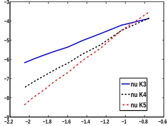
Subfigure 1(b) shows a 2-dimensional example. The data is generated by the smooth function

f(x) =sin(x1+x2) .

This function f is sampled on regular grids in the unit interval I := [0,1]2 _{with 16 to 144 points.}

Note that in this case the fill distance is given by h_≈√1

N. We use three different kernel functions,

namely (see Wendland, 2005)

• K3(x) = (1− kxk)4+(4kxk+1)with native space W22.5 [0,1]2

,

• K4(x) = (1− kxk)6₊35kxk2+18kxk+3

with native space W₂3.5 [0,1]2

, and

• K5(x) = (1_{− k}x_k)8₊32_kx_k3+25_kx_k2+8_kx_k+1

with native space W₂4.5 [0,1]2

.

The kernel functions were scaled by c=2 according to Equation (17). For the sake of simplicity we employed only theν-SVR with the parameter choices provided in Corollary 11. The predicted convergence rates in the fill distance h are 1.5 for K3, 2.5 for K4 and 3.5 for K5. The numerical

experiments show orders 1.8 for K3, 2.8 for K4and 3.7 for K5. Therefore, the numerical examples

support our analytical results.

−5.5 −5 −4.5 −4

−7.5 −7 −6.5 −6 −5.5 −5 −4.5 −4

eps K1 eps K2 nu K1 nu K2

(a) Data generated by f∈W₂3(I)on regular grids in I.ν -andε-SVR yield orders 1.7 for K1, and 2.4 for K2. Scaling parameter c=0.1.

−2.2 −2 −1.8 −1.6 −1.4 −1.2 −1 −0.8 −0.6 −9

−8 −7 −6 −5 −4 −3

nu K3 nu K4 nu K5

(b) Data generated by smooth function on regular grids in I2.ν-SVR yields orders 1.8 for K3, 2.8 for K4, and 3.7 for K5. Scaling parameter c=2.

Figure 1: Logarithm of the L∞-approximation error plotted versus the logarithm of the fill distance

h for exact training data.

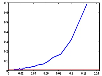
10.2 Inexact Data

Figure 2 shows examples for the case of noisy data. The plots show the L_∞-approximation error

kf₋sX,yk_L∞ versus the fill distance h. For simplicity we concentrated on the case of theν-SVR in

the one dimensional setting. We used the noise model given by Equation (14), that is y= f+r.

In Subfigure 2(a) the function f(x) =sin(10x) is sampled on regular grids of 2 to 56 points in

Corollary 14. The plot shows that for h→0 the error remains of the same order of magnitude as the error level_kr_kℓ∞.

In Subfigure 2(b) the function f(x) =sin(10x)is sampled on regular grids of 5 to 56 points in the unit interval I= [0,1]. Here, the data is corrupted by an error of±0.01, where the sign of the error is chosen randomly with equal likelihood for plus and minus. As kernel function we use K1 with c=0.3, and the parameters of theν-SVR are chosen as in Corollary 14. The plot shows that the L_∞ -approximation error converges to a constant of the order of magnitude of the error level for h_→0.

0 0.02 0.04 0.06 0.08 0.1 0.12 0.14 0.16 0

0.1 0.2 0.3 0.4 0.5 0.6 0.7

(a) Data disturbed by random error with mean zero and standard deviation 0.01. Approximation error for h→0 reaches the error level and remains bounded of the same order of magnitude as the error level.

0 0.02 0.04 0.06 0.08 0.1 0.12 0.14 0

0.1 0.2 0.3 0.4 0.5 0.6 0.7

(b) Data disturbed by random sign deterministic error ±0.01. Approximation error converges to a constant of the order of magnitude of the error level for h→0.

Figure 2: L_∞-approximation error versus fill distance in case of inexact data.

11. Summary and Outlook

We proved deterministic worst-case error estimates for kernel-based regression algorithms. The main ingredient are sampling inequalities. We provided a detailed analysis only for theν- and the

ε-SVR for both exact and inexact training data. However, the same techniques apply to all machine learning problems involving penalty terms induced by kernels related to Sobolev spaces. If the func-tion to be reconstructed lies in the reproducing kernel Hilbert space (RKHS) of an infinitely smooth kernel such as the Gaussian or an infinite dot product kernel, a similar analysis based on sampling inequalities can be done, leading to exponential convergence rates (see Rieger and Zwicknagl 2008 and Zwicknagl 2009 for first results in this direction).

So far, our error estimates depend explicitly on the pointwise noise in the data, and we do not make any assumptions on the noise distribution. Future work should incorporate probabilistic models on the noise distribution to yield estimates for the expected error.

Acknowledgments

We thank Professor Robert Schaback for helpful discussions and his continued support. Further thanks go to the referees for several valuable comments. CR was supported by the Deutsche Forschungsgemeinschaft through the Graduiertenkolleg 1023 Identification in Mathematical

Mod-els: Synergy of Stochastic and Numerical Methods. BZ would like to thank the German National

References

S.C. Brenner and L.R. Scott. The Mathematical Theory of Finite Element Methods, volume 15 of

Texts in Applied Mathematics. Springer, New York, 1994.

C-C. Chang and C-L. Lin. Trainingν-support vector regression: Theory and algorithms. Neural

Computation, 14(8):1959–1977, 2002.

T. Evgeniou, M. Pontil, and T. Poggio. Regularization networks and support vector machines.

Advances in Computational Mathematics, 13:1–50, 2000.

F. Girosi. An equivalence between sparse approximation and support vector machines. Neural

Computation, 10 (8):1455–1480, 1998.

C. A. Micchelli and M. Pontil. Learning the kernel function via regularization. Journal of Machine

Learning Research, 6:1099–1125, 2005.

C. Rieger and B. Zwicknagl. Sampling inequalities for infinitely smooth functions, with applications to interpolation and machine learning. To appear in Advances in Computational Mathematics, 2008.

M. Riplinger. Lernen als inverses Problem und deterministische Fehlerabschätzung bei Support Vektor Regression. Diplomarbeit, Universität des Saarlandes, 2007.

R. Schaback. The missing wendland functions. To appear in Advances in Computational

Mathe-matics, 2009.

B. Schölkopf and A.J. Smola. Learning with kernels - Support Vector Machines, Regularisation,

and Beyond. MIT Press, Cambridge, Massachusetts, 2002.

B. Schölkopf, C. Burges, and V.Vapnik. Extracting support data for a given task. In Proceedings,

First International Conference on Knowledge Discovery and Data Mining. CA:AAAI Press.,

Menlo Park, 1995.

B. Schölkopf, R.C. Wiliamson, and P.L. Bartlett. New support vector algorithms. Neural

Compu-tation, 12:1207–1245, 2000.

C.J. Stone. Optimal global rates of convergence for nonparametric regression. The Annals of

Statis-tics, 10:1040–1053, 1982.

V. Vapnik. The Nature of Statistical Learning Theory. Springer-Verlag, New York, 1995.

H. Wendland. Scattered Data Approximation. Cambridge Monographs on Applied and Computa-tional Mathematics. Cambridge University Press, Cambridge, 2005.

H. Wendland and C. Rieger. Approximate interpolation. Numerische Mathematik, 101:643–662, 2005.

J. Wloka. Partielle Differentialgleichungen: Sobolevräume und Randwertaufgaben. Mathematische Leitfäden. Teubner, Stuttgart, 1982.