assessing the severity degree of glaucoma and
the visual field loss
Koprowski
et al.
R E S E A R C H
Open Access
Automatic method of analysis of OCT images in
assessing the severity degree of glaucoma and
the visual field loss
Robert Koprowski
1*, Marek Rzendkowski
2and Zygmunt Wróbel
1* Correspondence: [email protected]
1Department of Biomedical
Computer Systems, Faculty of Computer Science and Materials Science, Institute of Computer Science, University of Silesia, ul. Będzińska 39, Sosnowiec 41-200, Poland
Full list of author information is available at the end of the article
Abstract
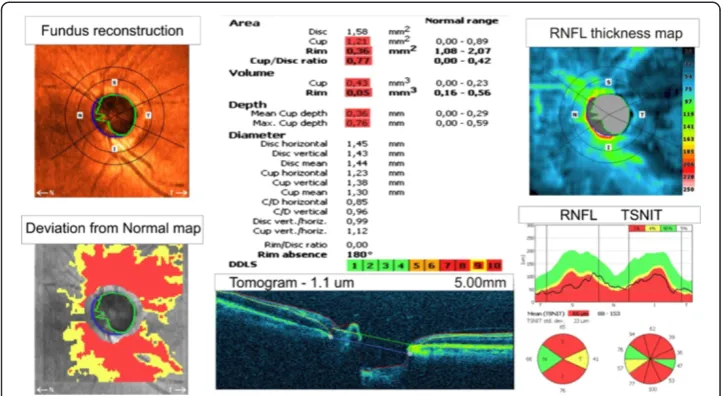
Introduction:In many practical aspects of ophthalmology, it is necessary to assess the severity degree of glaucoma in cases where, for various reasons, it is impossible to perform a visual field test - static perimetry. These are cases in which the visual field test result is not reliable, e.g. advanced AMD (Age-related Macular Degeneration). In these cases, there is a need to determine the severity of glaucoma, mainly on the basis of optic nerve head (ONH) and retinal nerve fibre layer (RNFL) structure. OCT is one of the diagnostic methods capable of analysing changes in both, ONH and RNFL in glaucoma.
Material and method:OCT images of the eye fundus of 55 patients (110 eyes) were obtained from the SOCT Copernicus (Optopol Tech. SA, Zawiercie, Poland). The authors proposed a new method for automatic determination of the RNFL (retinal nerve fibre layer) and other parameters using: mathematical morphology and profiled segmentation based on morphometric information of the eye fundus. A quantitative ratio of the quality of the optic disk and RNFL–BGA (biomorphological glaucoma advancement) was also proposed. The obtained results were compared with the results obtained from a static perimeter.
Results:Correlations between the known parameters of the optic disk as well as those suggested by the authors and the results obtained from static perimetry were calculated. The result of correlation with the static perimetry was 0.78 for the existing methods of image analysis and 0.86 for the proposed method. Practical usefulness of the proposed ratio BGA and the impact of the three most important features on the result were assessed. The following results of correlation for the three proposed classes were obtained: cup/disk diameter 0.84, disk diameter 0.97 and the RNFL 1.0. Thus, analysis of the supposed visual field result in the case of glaucoma is possible based only on OCT images of the eye fundus.
Conclusions:The calculations and analyses performed with the proposed algorithm and BGA ratio confirm that it is possible to calculate supposed mean defect (MD) of the visual field test based on OCT images of the eye fundus.
Keywords:Image processing, Measurement automation, OCT, Segmentation, BGA, Biomorphological glaucoma advancement, Glaucoma
Introduction
Analysis of OCT images of the eye fundus is a technique known for many years which enables to acquire large amounts of information useful for medical diagnosis. Today, there are many known profiled algorithms for the analysis of both successive layers of the eye fundus [1-20] as well as the choroid layer [21]. Depending on the approach and practical implementation, these algorithms operate in the area of texture analysis [1,2], algorithms based on segmentation with Canny method [4], SVM [5], mathematical morphology [6], active contour [7,8], fuzzy algorithms [9], Markov model [10], robust segmentation [11], random contour analysis [12] and others [13-20]. Implementation of these algorithms most commonly occurs in the C, C# programming environment if they are used in commercially available applications, or, for example, in Matlab if they are at the stage of testing and modification [6]. The analysis time of a single OCT image of the fundus is several tens of milliseconds to a few seconds with the most com-putationally intensive applications [1,17]. In practice, the biggest difficulty is large inter-individual variability and a possible high degree of retinal pathology. This translates into problems with the designation of successive layers of the eye fundus (RNFL–retinal nerve fibre layer, RPE–retinal pigment epithelium, and others) in the following cases (Figure 1):
The layer (u1,u3) is not continuous - Figure1a,d,
The layer (u2,u3) merges with another layer (u1) - Figure1b,
One layer ends (u1oru2) and another one starts (u3) in the same place - Figure1c.
Figure 1Diagrams showing problems during recognition of layers in an OCT image of the eye fundus.The following issues are shown in sequence:a)the problem with the gap betweenu1andu3and
the impact of the additional new layeru2,b)the problem with combining layersu2andu3with the layer u1for 3 pixels (1,4), (1,5) and (1,6),c)the difficulty in deciding which layeru1oru2should be combined
with the layeru3,d)the difficulty in deciding whether the layeru2is the missing piece connecting layersu1
The mentioned problems can be handled with in a limited way using artificial intelligence (knowledge gained from other images) or anthropometric evidence. In any case, image analysis and the proposed approach to solving such cases are difficult.
From a medical viewpoint, the RNFL thickness is essential in the case of the optic disk analysis. On the basis of its average thickness and further measurements, other parameters such as a cup/disk area ratio or a cup/disk vertical diameter are obtained. These parameters have an influence on the diagnosis of an ophthalmologist as well as the applied methods of treatment.
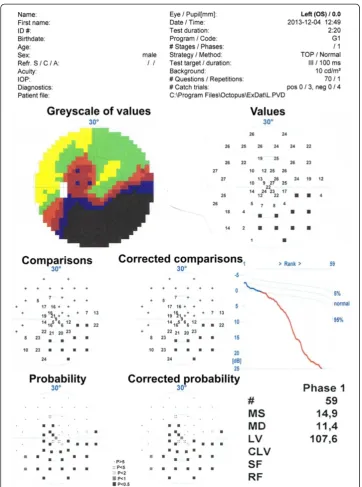
In the case of glaucoma, it is essential to test the visual field. Its measurement is usu-ally carried out using a static perimeter. A reliable parameter obtained from perimetric data is the average depth of a defect. In many cases, for example, in a number of differ-ent additional diseases, it is impossible to obtain this type of measuremdiffer-ent or the results obtained are not reliable. Then, it is necessary to search for other methods which will enable to determine the supposed visual field results. One such method is the analysis of OCT images of the eye fundus proposed by the authors. It allows not only to determine the severity degree of glaucoma but also to determine the supposed MD value of visual field test. It is further shown which selected parameters in OCT images correlate, to the greatest extent, with the results obtained from perimetry. Moreover, the new algorithm proposed by the authors and the quantitative ratio of the optic disk condition are described.
Material
OCT images of the eye fundus of 55 glaucoma patients (110 eyes) were obtained from the SOCT Copernicus (Optopol Tech. SA, Zawiercie, Poland). Patients ranged in age from 37 to 88 years. The obtained images (B-scans) had a resolution of M×N =1000 × 600 pixels (whereM –number of rows,N– number of columns) at a colour resolution of 8 bits/pixel. For each patientI =99 B-scans were obtained allowing for full 3D reconstruction of the eye fundus image. At the same time, 110 results were acquired from the static perimeter OCTOPUS 300Series V 6.07c. All data were analysed in a source format. The presented analysis was carried out retrospectively on the basis of data obtained during typical medical examinations. The data were anonymised and the patients were examined in accordance with the Declaration of Helsinki.
Methods
The method of analysis and processing of OCT images proposed by the authors was preceded by the analysis of the results obtained from conventional methods. This analysis indicates features which should be taken into account when constructing the target image analysis algorithm.
Selection of the features of the image
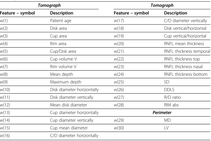
the features from w(1) to w(28) were acquired from the tomograph, and w(29) and w(30) from the perimeter. The parameters from w(1) to w(30) were further subjected to exploratory factor analysis in order to detect their cross correlation and to remove those features which are statistically insignificant. For this purpose, the following items were designated in succession: correlation of features w, eigenvalues of the correlation matrix, the number of classes using the Kaiser’s and Cattell’s criteria, rotation of the co-ordinate system, correlation of individual features with the newly created classes. The results (for the whole group of patients) are shown in Table 3 whereas the correlation chart of various features with three classes are shown in Figure 4. The analysis of Table 3 and Figure 4 suggests several conclusions useful for further analysis:
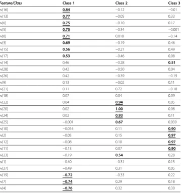
Class 1 significantly (above 0.5) correlates with the featuresw(16), w(13), w(6),w(5), w(8), w(3), w(15) and w(17) and is in a negative correlation with the features w(19), w(7) and w(4). It means that the cup/disk diameter and the cup diameter are a representative of the class 1. The ratio of the cup vertical/horizontal and the area and volume of the rim are in the inverse correlation.
Class 2 significantly correlates with the features w(22), w(20), w(24), w(25), w(23). These features are responsible for the RNFL parameters.
Class 3 correlates with the features w(10), w(2), w(12), w(11) and w(14) which are responsible for the parameters of the disk diameter in the vertical and hori-zontal axes.
Analysis of this division into classes, their correlation with the results obtained from perimetry and interpretation of individual features allow to specify the features of OCT images necessary for further analysis. The particularly important features of OCT image are: disk diameter and its relation to cup as well as the RNFL parameters in the area. This information is the basis for the design of a profiled image analysis algorithm, correlation analysis with the results of perimetry and for suggesting a new quantitative ratio of the optic disk condition.
Pre-processing
Pre-processing of images is related to automatic unpacking of the source file with the extension *.oct and thus acquiring images in the *.jpg format and calibration data. These data mainly include information recorded by the tomograph in the info.ini file, for example, the position of subsequent B-scans in space, the numbers
of A-scans and B-scans, date of test, the patient data and others. The sequence of images LGRAY(m,n,i) obtained on this basis is further subjected to filtration
with a median filter whose mask h1 is sized Mh1×Nh1× Ih1 =3 × 3 × 3 pixels. The
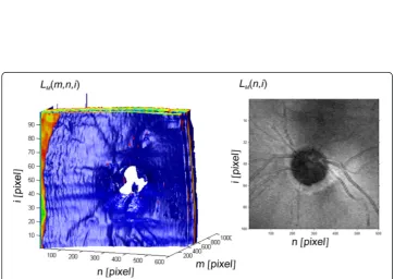
mask size was chosen arbitrarily taking into account the size of distortions and artefacts entering the optical path. The filtered image LM(m,n,i) (Figure 5) is
sub-jected to further preliminary transformations. These include determination of the RNFL.
Processing–RPE, ILM, RNFL, cup, disk
In order to determine the RNFL, the RPE layer (retinal pigment epithelium) is pre-determined automatically. The RPE layer is the most characteristic and the brightest layer in an OCT image, therefore, it is used to determine the target RNFL. Additionally, the RPE is used to determine the disk boundary. For this purpose, every n-th column of the imageLM, each A-scan, is analysed. Analogously to the method
described in [21,22], the position of the maximum brightness for each column is pre-determined, i.e.:
LRPEð Þ ¼n;i arg max
m∈ð1;MÞðLMðm;n;iÞÞ
ð1Þ
where:
m,n–coordinates of the rows and columns of the matrixm∈(1,M) andn∈(1,N). The formula (1) can be directly applied only when for all the analysed rows of each column there is only one maximum brightness value. As shown in [6], in practice it occurs in about 80% of the cases analysed at a resolution of 8 bits per pixel. On this
Table 1 Image features obtainable with the known software of the tomograph and the static perimeter
Tomograph Tomograph
Feature–symbol Description Feature–symbol Description
w(1) Patient age w(17) C/D diameter vertically
w(2) Disk area w(18) Disk vertical/horizontal
w(3) Cup area w(19) Cup vertical/horizontal
w(4) Rim area w(20) RNFL mean thickness
w(5) Cup/Disk area w(21) RNFL thickness temporal
w(6) Cup volume V w(22) RNFL thickness top
w(7) Rim volume V w(23) RNFL thickness nasal
w(8) Mean depth w(24) RNFL thickness bottom
w(9) Maximum depth w(25) SD
w(10) Disk diameter horizontally w(26) DDLS
w(11) Disk diameter vertically w(27) R/D ratio
w(12) Mean disk diameter w(28) RIM abs
w(13) Cup diameter horizontally Perimeter
w(14) Cup diameter vertically w(29) MD
w(15) Cup mean diameter w(30) LV
basis, two essential elements are calculated: disk and ILM layer. The disk location, the imageLdisk, is here calculated as the area:
Ldiskð Þ ¼n;i
1 if LRPEð Þn;i >pm⋅mean
n;i ðLRPEð Þn;iÞ
0 other (
ð2Þ
where: mean–mean value, pm–threshold equal 2/3.
The value of 2/3 (pm) was chosen arbitrarily and is associated with the
max-imum acceptable shift of the RPE layer in the area of the optic disk. The other element, namely the ILM layer area, was calculated as the area from the first pixel of each row to LRPE(n,i). It is very easy to perform binarization in this area using
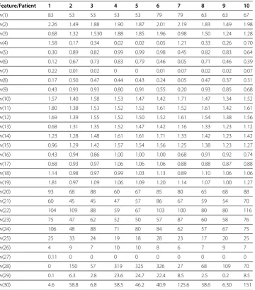
Table 2 Sample results for the first 10 patients obtained from the tomograph and perimeter
Feature/Patient 1 2 3 4 5 6 7 8 9 10
w(1) 83 53 53 53 53 79 79 63 63 67
w(2) 2.26 1.49 1.88 1.90 1.87 2.01 2.19 1.83 1.49 1.98
w(3) 0.68 1.32 1.530 1.88 1.85 1.96 0.98 1.50 1.24 1.28
w(4) 1.58 0.17 0.34 0.02 0.02 0.05 1.21 0.33 0.26 0.70
w(5) 0.30 0.89 0.82 0.99 0.99 0.98 0.45 0.82 0.83 0.64
w(6) 0.12 0.67 0.73 0.83 0.79 0.46 0.05 0.71 0.46 0.39
w(7) 0.22 0.01 0.02 0 0 0.01 0.07 0.02 0.02 0.07
w(8) 0.17 0.50 0.47 0.44 0.43 0.24 0.05 0.47 0.37 0.31
w(9) 0.43 0.93 0.93 0.80 0.91 0.55 0.20 0.93 0.85 0.68
w(10) 1.57 1.40 1.58 1.53 1.47 1.42 1.71 1.47 1.34 1.52
w(11) 1.80 1.38 1.53 1.52 1.52 1.61 1.52 1.61 1.42 1.61
w(12) 1.69 1.39 1.55 1.52 1.50 1.52 1.61 1.54 1.38 1.56
w(13) 0.68 1.31 1.35 1.52 1.47 1.42 1.16 1.33 1.23 1.12
w(14) 1.23 1.28 1.48 1.61 1.61 1.71 1.33 1.42 1.23 1.42
w(15) 0.96 1.29 1.42 1.57 1.54 1.56 1.25 1.38 1.23 1.27
w(16) 0.43 0.94 0.86 1.00 1.00 1.00 0.68 0.91 0.92 0.74
w(17) 0.68 0.93 0.97 1.06 1.06 1.06 0.88 0.88 0.87 0.88
w(18) 1.14 0.98 0.97 0.99 1.03 1.13 0.89 1.10 1.06 1.06
w(19) 1.81 0.97 1.09 1.06 1.09 1.20 1.14 1.07 1.00 1.27
w(20) 93 68 88 60 67 85 80 65 68 88
w(21) 60 45 45 47 57 86 67 59 54 70
w(22) 104 109 88 59 67 103 100 80 80 116
w(23) 75 47 62 52 50 57 87 60 58 76
w(24) 106 48 88 71 80 84 62 57 67 75
w(25) 25 33 24 19 18 28 23 17 20 25
w(26) 4 9 7 10 10 8 6 7 9 7
w(27) 0.11 0 0 0 0 0 0 0 0 0
w(28) 0 150 57 319 325 326 27 68 109 70
w(29) 0.1 6.3 2.8 23.6 24.7 22.4 8.5 2.5 0.2 8.5
Otsu method [23], thus setting the binarization threshold pr. The resulting binary
image LB(m,n,i) is:
LBðm;n;iÞ ¼
1 if ðLMðm;n;iÞ>prÞ∧ðm≤LRPEð Þn;i Þ
0 others
ð3Þ
Based on the binary imageLB(m,n,i), the edge of the ILM layer was defined as:
LSðm;n;iÞ ¼ m if LBðm;n;iÞ ¼1 M other
ð4Þ
LILMð Þ ¼n;i min
m∈ð1;MÞðLSðm;n;iÞÞ ð5Þ
The waveform of LILM(n,i) and the RPE boundary, i.e.LRPE(n,i), are the basis for
fur-ther analysis of the RNFL layer and cup area. The area between the layers ILM and RPE is further subjected to an operation which involves determination of the edge
Table 3 The results (for the whole group of patients) obtained from factor analysis for the three classes (bold >0.5, underlined >0.7)
Feature/Class Class 1 Class 2 Class 3
w(16) 0.84 −0.12 −0.01
w(13) 0.77 −0.05 0.33
w(6) 0.75 −0.10 0.17
w(5) 0.75 −0.34 −0.001
w(8) 0.71 0.018 −0.14
w(3) 0.69 −0.19 0.46
w(15) 0.56 −0.21 0.49
w(17) 0.53 −0.46 0.08
w(14) 0.46 −0.28 0.51
w(28) 0.42 −0.50 0.04
w(26) 0.42 −0.39 −0.19
w(9) 0.13 −0.02 0.11
w(21) 0.11 0.72 −0.18
w(18) 0.07 0.04 0.09
w(22) 0.04 0.94 0.05
w(20) 0.02 1.00 0.08
w(24) 0.02 0.93 0.11
w(25) −0.001 0.67 0.039
w(10) −0.014 0.11 0.90
w(2) −0.05 0.15 0.97
w(12) −0.08 0.10 0.97
w(11) −0.13 0.07 0.90
w(23) −0.19 0.54 0.28
w(1) −0.40 −0.31 0.15
w(27) −0.49 0.31 0.05
w(19) −0.72 −0.33 0.22
w(7) −0.74 0.29 0.18
Figure 4The result of factor analysis of 28 features and their division into 3 classes.Each of the 28 features is represented in this plot by a vector, and the direction and length of the vector indicate how each feature depends on the underlying factors (class). The orthogonal nature of the majority of the features, in particularw(16),w(22) tow(25) andw(1),w(2)w(12) as well asw(11), is clearly visible. Individual observations are marked in red. On the right side in the corners the characteristic areas have
been enlarged.
Figure 5The result of 3D reconstruction of the imageLM(m,n,i) and the imageLM(n,i).The first image
using two orthogonal Prewitt masks hh and hv sized 3 × 3 pixels. Filtration results in
the imageLG(m,n,i), i.e.:
LGðm;n;iÞ ¼
ffiffiffiffiffiffiffiffiffiffiffiffiffiffiffiffiffiffiffiffiffiffiffiffiffiffiffiffiffiffiffiffiffiffiffiffiffiffiffiffiffiffiffiffiffiffiffiffiffiffiffiffiffiffiffi LGhðm;n;iÞ2þLGvðm;n;iÞ2 q
if ðm>LILMð Þn;iÞ∧ðm<LRPEð Þn;iÞ
0 other
(
ð6Þ
where: LGh(m,n,i) and LGv(m,n,i) are the result of convolution of the image LM(m,n,i) with the maskshhandhv.
The RNFL is characterized by a contour visible in each column of the imageLM(m,n,i)
as a transition from a light area (below the ILM) to a dark one (the other layers). It is therefore the first edge below the ILM forLG(m,n,i) > 0, i.e. (analogously to (4), (5)):
LRðm;n;iÞ ¼ m if ðLGðm;n;iÞ>0Þ∧ðm>LILMð Þn;iÞ∧ðm<LRPEð Þn;i Þ M other
ð7Þ
LRNFLð Þ ¼n;i min
m∈ð1;MÞðLRðm;n;iÞÞ ð8Þ
The protection (m > LILM(n,i))∧(m < LRPE(n,i)) is additional and prevents
detec-tion of the RNFL on the edge of the analysed object with the background. The resulting edge has a number of disadvantages. The biggest one is the lack of con-tinuity caused by both occurring shadows as well as insufficient contrast in the place of its detection. For such cases, the method of active edge correction was suggested. This method involves adjustment of the position of the layer LRPE(n,i).
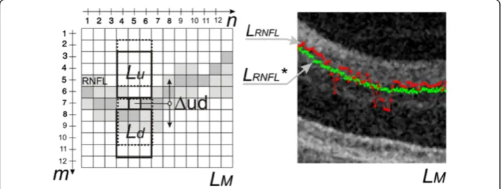
For each point of the layer LRPE(n,i), the mean brightness value above and below
LRPE(n,i) in the areas Lu and Ld is determined - Figure 6. The new corrected
pos-ition of the layer LRPE*(n,i) is determined as the maximum difference between the
average values in the areas Lu(Δud,n,i) and Ld(Δud,n,i). These areas are shifted in
Figure 6The results of the dynamic adjustment of the contour position.On the left side, the idea of the dynamic contour position adjustment has been shown. The difference between the mean values in the areasLuandLdprovides information about the correct position of the point. The greatest difference
between the areasLuandLdis searched for in a selected area. The right side shows an example of the
the column axis in the range Δud =±med(|LILM(n,i)-LRPE(n,i)|). The adjusted
pos-ition of the RNFL is therefore calculated as:
LRNFLð Þ ¼n;i arg
m
max
Δud ðjLuðΔud;n;iÞ−LdðΔud;n;iÞjÞ
ð9Þ
The resulting new position of the layerLRNFL*(n,i) is the basis for further analysis. On
the basis of the positions of the ILM and RPE layers, i.e.: LILM(n,i), LRPE(n,i), the cup
area Lcup(n,i) is determined. This area is calculated as the intersection of the boundary
ofLdisk(n,i) at the offset height equal to 150μm with the layerLILM(n,i).
As evident from the exploratory factor analysis presented in the previous section, apart from the RNFL thickness, also limitation of the analysis area - ROI (region of interest) is vital. The ROI ranges from 2∙rdisk to 3∙rdisk in an OCT image and in
order to determine it, it is necessary to determine the position of coordinates of the centre (nd0,id0), i.e.:
nd0¼
XI
i¼1
XN
n¼1ðLdiskð Þn;i⋅nÞ
XI
i¼1
XN
n¼1Ldiskð Þn;i
ð10Þ
id0¼ XI
i¼1 XN
n¼1ðLdiskð Þn;i ⋅iÞ XI
i¼1 XN
n¼1Ldiskð Þn;i
ð11Þ
The value ofrdiskis the average radius calculated from the area of a circle:
rdisk¼
ffiffiffiffiffiffiffiffiffiffiffiffiffiffiffiffiffiffiffiffiffiffiffiffiffiffiffiffiffiffiffiffiffiffiffiffiffiffiffiffiffiffiffiffi XI
i¼1 XN
n¼1Ldiskð Þn;i π
s
ð12Þ
The calculation of the centre of gravity is followed by the conversion of the ROI to the polar coordinate system, i.e.:
θ¼atan2ðn−nd0;i−id0Þ ð13Þ
ρ¼ ffiffiffiffiffiffiffiffiffiffiffiffiffiffiffiffiffiffiffiffiffiffiffiffiffiffiffiffiffiffiffiffiffiffiffiffiffiffiffiðn−nd0Þ2þði−id0Þ2 q
ð14Þ
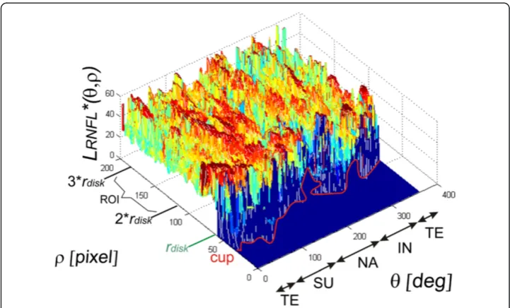
The function atan2 returns θ the same size as n and i containing the element-by-element, four-quadrant inverse tangent (arctangent) of the real parts of n and i. The obtained results, the ROI in the polar coordinate system LRNFL*(θ,ρ), are shown in
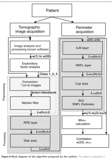
Figure 7. The proposed algorithm is shown globally in a block diagram form in Figure 8. On the basis of the presented ROI, the following results (features) were obtained: the disk diameter and its relation to the cup and RNFL parameters. Their thorough analysis and correlation with the results from perimetry are pre-sented in the next section.
Results
The obtained result LRNFL*(θ,ρ), the ROI in the polar coordinate system (Figure 7), is
different classes (Figure 4, Table 3), associated with LRNFL*(θ,ρ), were formulated
in the following way:
wg(1)–the relative difference in the positions of centres of gravity calculated as:
wgð Þ ¼1
ffiffiffiffiffiffiffiffiffiffiffiffiffiffiffiffiffiffiffiffiffiffiffiffiffiffiffiffiffiffiffiffiffiffiffiffiffiffiffiffiffiffiffiffiffi nd0−nc0
ð Þ2þ
id0−ic0
ð Þ2
q
rdisk ð
15Þ
where:
nd0, id0–coordinates of the centre of gravity of the disk,
nc0, ic0–coordinates of the centre of gravity of the cup,
wg(2) – relative, inverse, minimum distance between the boundaries of the cup and
disk i.e.:
wgð Þ ¼2 1− rmin
rdisk ð
16Þ
where:rmin–minimum distance between the boundaries of the cup and disk.
wg(3) – RNFL thickness deviation in the ROI (LRNFLROI(θ)) for particular areas:
temporal (TM), superior (SU), nasal (NA), interior (IN) from the standard thick-ness changes:
wgð Þ ¼3
1 360
X
θ
LROI
RNFLð Þθ −LWZRNFLð Þθ LWZ
RNFLð Þθ
ð17Þ
where: LRNFLWZ(θ)–the reference value of the RNFL thickness (the graph highlighted in green in Figure2).
The mentioned features are components of the proposed biomorphological glaucoma advancement ratio (BGA) which is defined as:
Figure 8Block diagram of the algorithm proposed by the authors.The patient undergoes a fundus examination with the use of a tomograph and their visual field is measured with a perimeter. Then, the significance and correlation of the features obtained are calculated, thereby forming three classes. They are the basis for proposing a new analysis algorithm. After automatic determination of the layers RPE, ILM, RNFL and the cup and disk, the featureswg(1), wg(2) andwg(3) are determined.
wBGA¼
1
3⋅ wgð Þ þ1 wgð Þ þ2 wgð Þ3
ð18Þ
After value substitution and simplification:
wBGA¼
ffiffiffiffiffiffiffiffiffiffiffiffiffiffiffiffiffiffiffiffiffiffiffiffiffiffiffiffiffiffiffiffiffiffiffiffiffiffiffiffiffiffiffiffiffi nd0−nc0
ð Þ2þ
id0−ic0
ð Þ2
q
þrdisk−rmin
3⋅rdisk þ
wgð Þ3
3 ð19Þ
Figure 9 presents a list of various types of cup arrangements relative to the disk and the impact of their sizes on the values of the features wg(1), wg(2) andwg(3) as well as
wBGA. In addition, for comparison, the values of the DDLS (Disk Damage Likelihood
Scale) were also shown [24]. A change in the position of the centre of gravity of the cup relative to the disk is expressed by the featurewg(1). The closer the centres of
grav-ity of the cup are to each other, the closer the feature wg(1) is to zero. If the centres of
gravity of the cup and disk are far apart, the extreme position of the cup is on the edge of the disk, then the value of wg(1) is close to one. In turn, the featurewg(2) is a
meas-ure of centricity of the distribution of cup edges relative to the disk. When the edge of
Figure 9The impact of cup arrangement with respect to the disk on the valueswgandwBGA.
A summary of various typical cup arrangements relative to the disk and the effect of their size on the featureswg(1),wg(2) andwg(3) as well aswBGAand, in addition, the values of the DDLS, have been shown.
A change in the position of the cup centre of gravity relative to the disk is expressed by the featurewg(1).
the cup is substantially spaced from the edge of the disk, the value ofwg(2) is close to
zero. When the edges of the cup and the disk overlap in any area, then the value of wg(2) is close to one. The situation is similar in the case of advanced glaucoma where
rminis close to zero andwg(2) is close to one. A change in the value ofwg(3) is related
to a deviation with respect to the standard waveform of the RNFL thickness (Figure 2). The greater this difference is, the larger the value of wg(3) is, and vice versa. The
featureswg(1),wg(2) andwg(3) are summed up and thus determine the ratiowBGA.The
ratio wBGAreaches values close to one if all three featureswgindicate pathology. In the
case of the right featureswg, the ratiowBGAis equal to zero.
Based on the proposed ratio wBGA, its correlation with the results of perimetry was
determined. In addition, it was compared with the results obtained only on the basis of known software (featuresw(1) tow(29)). The following results were obtained:
Correlation of classes 1, 2, 3 (obtained from featuresw(1) tow(29)) with the results obtained from perimetry is 0.78,
Correlation of the proposed ratiowBGAreferred to the described method of image analysis and processing with the results of perimetry is 0.86–Figure10. The function describing the dependence ofw(29) (denoting the MD value from perimetry) onwBGAtakes the following form:
wð Þ ¼29 24⋅wBGA−9:34 ð20Þ
The difference in the correlation results stems from the profiled method of image analysis and processing and the measurement methodology of the described issue.
Figure 10Graph of the dependence ofw(29) as a function of changes in the ratiowBGA.The graph
shows in blue the results obtained for individual patients. The result of linear regression is marked in green. The function describing the dependence ofw(29) onwBGAtakes the following form:w(29) = 24⋅wBGA–9.34.
Summary
The paper presents a new methodology for image analysis and processing profiled for the optic disk analysis with a particular emphasis on its correlation with static perim-etry. The calculations and analyses performed with the proposed algorithm confirm the possibility of prediction of the visual field result based on OCT images of the eye fun-dus. The analysis time of a single OCT image of the eye fundus with the use of the pro-posed algorithm on the computer Core i5 CPU M460 @ 2.5GHz 4GB RAM does not exceed 0.2 s. Additionally, a new ratio reliable with respect to the quantitative assess-ment of the optic disk condition was proposed. On its basis, a comparison of the results of the correlation between the known methods and the methodology described in this paper was made.
The present paper does not exhaust this interesting subject. The proposed method of image analysis and processing is one of the possible approaches to solving this type of task. Certainly, other methods of image analysis and processing can be used here [25,26] such as texture analysis [27,28] or other methods applied to solving similar issues [29-31].
In further studies, the authors intend to test practical usefulness of the proposed algorithm and the ratio wBGA. The results obtained for large inter-individual variability
(diversity of shapes and topology of the optic disk), repeatability of the data and the impact of technological diversity and device parameters (tomograph and perimeter) on the result are particularly vital here.
Abbreviations
AMD:Age-related macular degeneration; ROI: Region of interest; RNFL: Retinal nerve fiber layer; TE: Temporal; SU: Superior; NA: Nasal; IN: Inferior; BGA: Biomorphological glaucoma advancement; MD: Mean defect; LV: Loss variance.
Competing interests
The authors declare that they have no competing interests.
Authors’contributions
RK suggested the algorithm for image analysis and processing, implemented it and analyzed the images. MR, ZW performed the acquisition of the tomography images and consulted the obtained results. All authors have read and approved the final manuscript.
Acknowledgements
No outside funding was received for this study.
Author details
1Department of Biomedical Computer Systems, Faculty of Computer Science and Materials Science, Institute of
Computer Science, University of Silesia, ul. Będzińska 39, Sosnowiec 41-200, Poland.2Individual Specialist Medical
Practice, Gliwice, Poland.
Received: 4 January 2014 Accepted: 10 February 2014 Published: 14 February 2014
References
1. Quellec G, Lee K, Dolejsi M, Garvin MK, Abràmoff MD, Sonka M:Three-dimensional analysis of retinal layer texture: identification of fluid-filled regions in SD-OCT of the macula.IEEE Trans Med Imaging2010,29(6):1321–1330. 2. KajićV, Povazay B, Hermann B, Hofer B, Marshall D, Rosin PL, Drexler W:Robust segmentation of intraretinal
layers in the normal human fovea using a novel statistical model based on texture and shape analysis.Opt Express2010,18(14):14730–14744.
3. Park SY, Kim SM, Song YM, Sung J, Ham DI:Retinal thickness and volume measured with enhanced depth imaging optical coherence tomography.Am J Ophthalmol2013,156(3):557–566.
4. Koprowski R, Wrobel Z:Identification of layers in a OCT image of an eye based on the canny edge detection. Inf Technol Biomed Adv Intell Soft Comput2008,47:232–239.
5. Wang S, Zhu WY, Liang ZP:ShapeDeformation: SVM regression and application to medical image segmentation.Eight Int Conf Comput Vis2001,2:209–216.
7. Yazdanpanah A, Hamarneh G, Smith B, Sarunic M:Intra-retinal layer segmentation in optical coherence tomography using an active contour approach.Med Image Comput Comput Assist Interv2009,12(2):649–656. 8. Yezzi A, Tsai A, Willsky A:A Statistical Approach to Snakes for Bimodal and Trimodal Imagery, Proceedings of the
seventh IEEE international conference on computer vision. Washington, DC: IEEE Computer Society; 1999:898–903. 9. Mayer MA, Tornow RP, Bock R, Hornegger J, Kruse FE:Automatic nerve fiber layer segmentation and geometry
correction on spectral domain OCT images using fuzzy C-means clustering.Invest Ophthalmol Vis Sci1880, 2008:49.
10. Koozekanani D, Boyer KL, Roberts C:Retinal thickness measurements in optical coherence tomography using a Markov boundary model.Med Imaging IEEE Trans2001,20(9):900–916.
11. Gregori G, Knighton RW:A robust algorithm for retinal thickness measurements using optical coherence tomography (stratus OCT).Invest Ophthalmol Vis Sci2004,45:3007.
12. Koprowski R, Wróbel Z:Layers recognition in OCT eye image based on random contour analysis. Computer recognition systems 3.Adv Intell Soft Comput2009,57:471–478.
13. Shahidi M, Wang Z, Zelkha R:Quantitative thickness measurement of retinal layers imaged by optical coherence tomography.Am J Ophthalmol2005,139(6):1056–1061.
14. Mujat M, Chan R, Cense B, Park B, Joo C, Akkin T, Chen T, Boer J:Retinal nerve fiber layer thickness map determined from optical coherence tomography images.Opt Express2005,13(23):9480–9491.
15. Mishra A, Wong A, Bizheva K, Clausi DA:Intra-retinal layer segmentation in optical coherence tomography images.Opt Express2009,17(26):23719–23728.
16. Lu S, Cheung C, Liu J, Lim S, Leung C, Wong T:Automated layer segmentation of optical coherence tomography images.IEEE Trans Biomed Eng2010,57(10):2605–2608.
17. DeBuc C, Somfai GM:Early detection of retinal thickness changes in diabetes using optical coherence tomography.Med Sci Monit2010,16(3):MT15–MT21.
18. Haeker M, Abràmoff M, Kardon R, Sonka M:Segmentation of the surfaces of the retinal layer from OCT images. Med Image Comput Comput Assist Interv2006,9(1):800–807.
19. Ishikawa I, Stein DM, Wollstein G, Beaton S, Fujimoto JG, Schuman JS:Macular segmentation with optical coherence tomography.Invest Ophthalmol Vis Sci2005,46(6):2012–2017.
20. Hu Z, Abramoff MD, Kwon YH, Lee K, Garvin M:Automated segmentation of neural canal opening and optic Cup in 3-D spectral optical coherence tomography volumes of the optic nerve head.Invest Ophthalmol Vis Sci 2010,51(11):5708–5717.
21. Koprowski R, Teper S, Wrobel Z, Wylegala E:Automatic analysis of selected choroidal diseases in OCT images of the eye fundus.Biomed Eng Online2013,12:117.
22. Koprowski R, Teper S, Weglarz B, Wylęgała E, Krejca M, Wróbel Z:Fully automatic algorithm for the analysis of vessels in the angiographic image of the eye fundus.Biomed Eng Online2012,11:35.
23. Otsu N:A threshold selection method from gray-level histograms.IEEE Trans Sys Man Cyber1979,9(1):62–66. 24. Wei H, Zangalli C, Spaeth GL:Valid estimation of the appearance of the optic nerve: the case against using
Cup/disk ratios.J Curr Glaucoma Pract2010,4(3):133–136.
25. Sonka M, Michael Fitzpatrick J:Medical Image Processing and Analysis, Handbook of Medical Imaging. Belligham: SPIE; 2000.
26. Tadeusiewicz R, Ogiela MR:Automatic understanding of medical images new achievements in syntactic analysis of selected medical images.Biocybern Biomed Eng2002,22(4):17–29.
27. Korzynska A, Zychowicz M:A method of estimation of the cell doubling time on basis of the cell culture monitoring data.Biocybern Biomed Eng2008,28(4):75–82.
28. Korzynska A, Iwanowski M:Multistage morphological segmentation of bright-field and fluorescent microscopy images.Opt-Electron Rev2012,20(2):87–99.
29. Siedlecki D, Nowak J, Zajac M:Placement of a crystalline lens and intraocular lens: retinal image quality. J Biomed Opt2006,11(5):054012.
30. Porwik P:Efficient spectral method of identification of linear Boolean function.Control Cybern2004,33(4):663–678. 31. Korus P, Dziech A:Efficient method for content reconstruction with self-embedding.IEEE Trans Image Process
2013,22(3):1134–1147.
doi:10.1186/1475-925X-13-16
Cite this article as:Koprowskiet al.:Automatic method of analysis of OCT images in assessing the severity degree of glaucoma and the visual field loss.BioMedical Engineering OnLine201413:16.
Submit your next manuscript to BioMed Central and take full advantage of:
• Convenient online submission
• Thorough peer review
• No space constraints or color figure charges
• Immediate publication on acceptance
• Inclusion in PubMed, CAS, Scopus and Google Scholar
• Research which is freely available for redistribution