University of New Orleans University of New Orleans
ScholarWorks@UNO
ScholarWorks@UNO
University of New Orleans Theses and
Dissertations Dissertations and Theses
5-14-2010
Representative Environments for Reduced Estimation Time of
Representative Environments for Reduced Estimation Time of
Wide Area Acoustic Performance
Wide Area Acoustic Performance
Josette Fabre
University of New Orleans
Follow this and additional works at: https://scholarworks.uno.edu/td
Recommended Citation Recommended Citation
Fabre, Josette, "Representative Environments for Reduced Estimation Time of Wide Area Acoustic Performance" (2010). University of New Orleans Theses and Dissertations. 1156.
https://scholarworks.uno.edu/td/1156
This Dissertation is protected by copyright and/or related rights. It has been brought to you by ScholarWorks@UNO with permission from the rights-holder(s). You are free to use this Dissertation in any way that is permitted by the copyright and related rights legislation that applies to your use. For other uses you need to obtain permission from the rights-holder(s) directly, unless additional rights are indicated by a Creative Commons license in the record and/ or on the work itself.
Representative Environments for Reduced Estimation Time of Wide Area Acoustic Performance
A Dissertation
Submitted to the Graduate Faculty of the University of New Orleans in partial fulfillment of the requirements for the degree of
Doctor of Philosophy in
Engineering and Applied Science Physics
by
Josette Paquin Fabre
B.S. Millsaps College, 1988 M.S. University of New Orleans, 1996
ii
Dedication
This dissertation is dedicated to the memory of my father, Dr. James E. Paquin. His
positive attitude, appreciation for all the good in the world, his extreme wisdom and his sense of
humor have influenced and guided me throughout my life.
iii
Acknowledgements
The author acknowledges and appreciates the sponsorship of the Office of Naval
Research (ONR) and SPAWAR PEO-C4I PMW-120.
The author would like to thank the following people for their help and many helpful
technical discussions: Dr. Stanley Chin-Bing, Dr. Michael Porter, Dr. Robert Zingarelli, Dr.
David King, Dr. Frank Bub, Richard Keiffer, David Fabre, Tracy Hall, Steven Dennis, Dr. James
Fulford, Dr. Joe Murphy, Dr. Juliette Ioup, Dr. Maria Kalcic, and Dr. George Ioup.
Finally, the author truly appreciates all the support and encouragement from David,
iv
Table
of
Contents
Table of Figures ... vi
Acronym List ... xvii
Abstract ... xix
Chapter 1. Introduction ... 1
Transmission of Sound through the Ocean ... 1
Overall Acoustic Provincing Concept ... 4
Chapter 2. Method ... 6
Environmental Acoustic Provincing Overview ... 6
Environmental Characterization ... 9
Acoustic Modeling ... 10
Acoustic Performance Estimates ... 11
Characterizing Uncertainty ... 12
Integrated Acoustic Multi-environmental Processing System (IAMPS) ... 13
Environmental Acoustic Factors Provincing ... 16
Mathematical Clustering ... 20
Environmental Parameter (Xi or ξ) Provincing ... 28
Derivation of ξ ... 28
Preliminary Acoustic Mode Bundling ... 32
Range Dependent ξ ... 37
Chapter 3. Results ... 38
Critical Factors Provincing ... 38
Okinawa Trough ... 38
Hawaii ... 82
v
Uncertainty Band Results for Provinces ... 113
Environmental Parameter (Xi or ξ) Range Independent Provincing ... 118
Chapter 4. Applications ... 127
Multiple Scenarios ... 127
Time Series ... 127
Integrated Signal Excess ... 128
High Resolution Radial ... 132
Chapter 5. Conclusions ... 134
References ... 136
Appendix - Glossary ... 141
vi
Table
of
Figures
Figure 1. Six grid points (3x2), with 8 radials each, for the brute-force option results in 48
acoustic runs... 8
Figure 2. Illustration of the provincing concept for the 3x2 example. Nine acoustic provinces are computed, so 9 acoustic computations will be done using the centroid environment, that is the environment closest to the center of the province. ... 9
Figure 3. Acoustic coverage concept, after Fabre, 2007. ... 12
Figure 4. Examples of the UBAND algorithm from Zingarelli and Fabre (2009) for an up-slope case at two frequencies. For the higher frequency case (left) the uncertainties increase as the sound travels up the slope. At the lower frequency (right), the energy falls off before the uncertainty gets too high. ... 13
Figure 5. Modeled transmission loss for a source in a sonic layer. The green curve represents the loss for a flat surface, the black curve represents the loss for which the more realistic rough surface was included in the modeling. The yellow curve was generated using a research surface loss model (Norton and Novarini, 1996). ... 18
Figure 6. Modeled TL for case shown in Figure 5, but with the more realistic 17m/s wind speed. The green curve represents the loss for a flat surface, the black curve represents the loss for which the more realistic rough surface was included in the modeling. The yellow curve was generated using a research surface loss model (Norton and Novarini, 1996). ... 20
Figure 7. Example of acoustic modes versus range for a single acoustic mode province. ... 21
Figure 8. TL for the mode province shown in Figure 7. ... 22
Figure 9. The SLD parameter (Baker, 1975) versus range for the mode province shown in Figure 7... 23
Figure 10. Example of sonic layer sub-province for a single acoustic mode province. ... 24
Figure 11. Subprovince of province 45 based on SLD. ... 24
Figure 12. TL for the sub-province shown in Figure 10. ... 25
Figure 13. Mode cost function for a province with 105 members. ... 26
vii
Figure 15. TL predictions at 15 m for each member of the sub-province shown in Figure 14. The
black line is the representative that is used to estimate the PAC in the provinced performance
prediction. ... 27
Figure 16. TL predictions at 150 m for each member of the sub-province shown in Figure 14.
The black line is the representative that is used to estimate the PAC in the provinced
performance prediction. ... 27
Figure 17. Mode bundling illustration. ... 32
Figure 18. Example Bellhop decimated raytrace for a deep water test case, with a source at 15 m.
Blue rays hit the bottom only, cyan rays hit the surface only and red are the volume rays. ... 34
Figure 19. ξ as a function of wavenumber (k) and depth (m). ... 35
Figure 20. ξ after being grouped into volume, surface and bottom interacting "bundles", and reduced to the fixed depths. ... 36
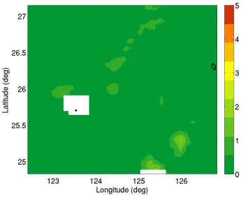
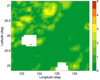
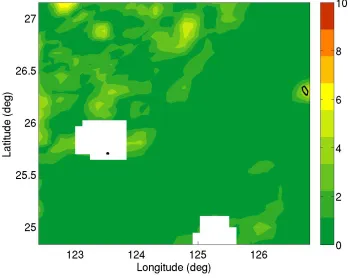
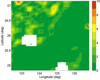
Figure 21. DBDB-V bathymetry in m for the Okinawa Trough area of interest. ... 39
Figure 22. Sonic layer depth in m (left) and cutoff frequency in Hz (right) for Okinawa Trough
area of interest. ... 39
Figure 23. Low frequency mode provinces for the Okinawa Trough area. ... 41
Figure 24. Brute force (left) and critical factors representative environment (right) PAC for 250
Hz, source at 15 m, receiver at 10 m. ... 42
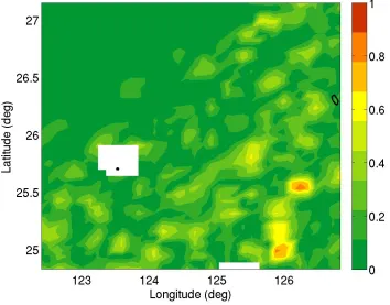
Figure 25. Averaged difference in percent between brute force and critical factors representative
environment PAC for 250 Hz, source at 15 m, receiver at 10 m. ... 42
Figure 26. Brute force (left) and critical factors representative environment (right) PAC for 250
Hz, source at 15 m, receiver at 15 m. ... 43
Figure 27. Averaged difference in percent between brute force and critical factors representative
environment PAC for 250 Hz, source at 15 m, receiver at 15 m. ... 43
Figure 28. Brute force (left) and critical factors representative environment (right) PAC for 250
Hz, source at 15 m, receiver at 20 m. ... 44
Figure 29. Averaged difference in percent between brute force and critical factors representative
environment PAC for 250 Hz, source at 15 m, receiver at 20 m. ... 44
Figure 30. Brute force (left) and critical factors representative environment (right) PAC for 250
viii
Figure 31. Averaged difference in percent between brute force and critical factors representative
environment PAC for 250 Hz, source at 15 m, receiver at 150 m. ... 45
Figure 32. Brute force (left) and critical factors representative environment (right) PAC for 250
Hz, source at 15 m, receiver at 250 m. ... 46
Figure 33. Averaged difference in percent between brute force and critical factors representative
environment PAC for 250 Hz, source at 15 m, receiver at 250 m. ... 46
Figure 34. Brute force (left) and critical factors representative environment (right) PAC for 250
Hz, source at 60 m, receiver at 10 m. ... 47
Figure 35. Averaged difference in percent between brute force and critical factors representative
environment PAC for 250 Hz, source at 60 m, receiver at 10 m. ... 47
Figure 36. Brute force (left) and critical factors representative environment (right) PAC for 250
Hz, source at 60 m, receiver at 15 m. ... 48
Figure 37. Averaged difference in percent between brute force and critical factors representative
environment PAC for 250 Hz, source at 60 m, receiver at 15 m. ... 48
Figure 38. Brute force (left) and critical factors representative environment (right) PAC for 250
Hz, source at 60 m, receiver at 20 m. ... 49
Figure 39. Averaged difference in percent between brute force and critical factors representative
environment PAC for 250 Hz, source at 60 m, receiver at 20 m. ... 49
Figure 40. Brute force (left) and critical factors representative environment (right) PAC for 250
Hz, source at 60 m, receiver at 150 m. ... 50
Figure 41. Averaged difference in percent between brute force and critical factors representative
environment PAC for 250 Hz, source at 60 m, receiver at 150 m. ... 50
Figure 42. Brute force (left) and critical factors representative environment (right) PAC for 250
Hz, source at 150 m, receiver at 10 m. ... 51
Figure 43. Averaged difference in percent between brute force and critical factors representative
environment PAC for 250 Hz, source at 150 m, receiver at 10 m. ... 51
Figure 44. Single point (01) representative analysis for 250Hz, source at 15 m, receiver at 10 m.
... 54
Figure 45. Single point (01b) representative analysis for 250Hz, source at 15 m, receiver at 15 m.
ix
Figure 46. Single point (04b) representative analysis for 250 Hz, source at 60 m, receiver at 20
m, after re-provincing of large provinces was added. ... 55
Figure 47. Single point (05) representative analysis for 250 Hz, source at 60 m, receiver at 20 m
after re-provincing of large provinces was added. ... 56
Figure 48. Brute force (left) and critical factors representative environment (right) PAC for 1000
Hz, source at 20 m, receiver at 10 m. ... 58
Figure 49. Averaged difference in percent between brute force and critical factors representative
environment PAC for 1000 Hz, source at 20 m, receiver at 10 m. ... 58
Figure 50. Brute force (left) and critical factors representative environment (right) PAC for 1000
Hz, source at 20 m, receiver at 15 m. ... 59
Figure 51. Averaged difference in percent between brute force and critical factors representative
environment PAC for 1000 Hz, source at 20 m, receiver at 15 m. ... 59
Figure 52. Brute force (left) and critical factors representative environment (right) PAC for 1000
Hz, source at 20 m, receiver at 20 m. ... 60
Figure 53. Averaged difference in percent between brute force and critical factors representative
environment PAC for 1000 Hz, source at 20 m, receiver at 20 m. ... 60
Figure 54. Brute force (left) and critical factors representative environment (right) PAC for 1000
Hz, source at 20 m, receiver at 150 m. ... 61
Figure 55. Averaged difference in percent between brute force and critical factors representative
environment PAC for 1000 Hz, source at 20 m, receiver at 150 m. ... 61
Figure 56. Brute force (left) and critical factors representative environment (right) PAC for 1000
Hz, source at 20 m, receiver at 200 m. ... 62
Figure 57. Averaged difference in percent between brute force and critical factors representative
environment PAC for 1000 Hz, source at 20 m, receiver at 200 m. ... 62
Figure 58. Brute force (left) and critical factors representative environment (right) PAC for 1000
Hz, source at 80 m, receiver at 10 m. ... 63
Figure 59. Averaged difference in percent between brute force and critical factors representative
environment PAC for 1000 Hz, source at 80 m, receiver at 10 m. ... 63
Figure 60. Brute force (left) and critical factors representative environment (right) PAC for 1000
x
Figure 61. Averaged difference in percent between brute force and critical factors representative
environment PAC for 1000 Hz, source at 80 m, receiver at 15 m. ... 64
Figure 62. Brute force (left) and critical factors representative environment (right) PAC for 1000
Hz, source at 80 m, receiver at 20 m. ... 65
Figure 63. Averaged difference in percent between brute force and critical factors representative
environment PAC for 1000 Hz, source at 80 m, receiver at 20 m. ... 65
Figure 64. Brute force (left) and critical factors representative environment (right) PAC for 1000
Hz, source at 80 m, receiver at 150 m. ... 66
Figure 65. Averaged difference in percent between brute force and critical factors representative
environment PAC for 1000 Hz, source at 80 m, receiver at 150 m. ... 66
Figure 66. Brute force (left) and critical factors representative environment (right) PAC for 1000
Hz, source at 80 m, receiver at 200 m. ... 67
Figure 67. Averaged difference in percent between brute force and critical factors representative
environment PAC for 1000 Hz, source at 80 m, receiver at 200 m. ... 67
Figure 68. Single point (06) representative analysis for 1000Hz, source at 20 m, receiver at 15 m.
... 69
Figure 69. Single point (07) representative analysis for 1000Hz, source at 20 m, receiver at 15 m.
... 70
Figure 70. Brute force (left) and critical factors representative environment (right) PAC for 3000
Hz, source at 15 m, receiver at 10 m. ... 72
Figure 71. Averaged difference in percent between brute force and critical factors representative
environment PAC for 3000 Hz, source at 15 m, receiver at 10 m. ... 72
Figure 72. Brute force (left) and critical factors representative environment (right) PAC for 3000
Hz, source at 15 m, receiver at 15 m. ... 73
Figure 73. Averaged difference in percent between brute force and critical factors representative
environment PAC for 3000 Hz, source at 15 m, receiver at 15 m. ... 73
Figure 74. Brute force (left) and critical factors representative environment (right) PAC for 3000
Hz, source at 15 m, receiver at 20 m. ... 74
Figure 75. Averaged difference in percent between brute force and critical factors representative
xi
Figure 76. Brute force (left) and critical factors representative environment (right) PAC for 3000
Hz, source at 15 m, receiver at 150 m. ... 75
Figure 77. Averaged difference in percent between brute force and critical factors representative
environment PAC for 3000 Hz, source at 15 m, receiver at 150 m. ... 75
Figure 78. Brute force (left) and critical factors representative environment (right) PAC for 3000
Hz, source at 15 m, receiver at 200 m. ... 76
Figure 79. Averaged difference in percent between brute force and critical factors representative
environment PAC for 3000 Hz, source at 15 m, receiver at 200 m. ... 76
Figure 80. Brute force (left) and critical factors representative environment (right) PAC for 3000
Hz, source at 60 m, receiver at 10 m. ... 77
Figure 81. Averaged difference in percent between brute force and critical factors representative
environment PAC for 3000 Hz, source at 60 m, receiver at 10 m. ... 77
Figure 82. Brute force (left) and critical factors representative environment (right) PAC for 3000
Hz, source at 60 m, receiver at 15 m. ... 78
Figure 83. Averaged difference in percent between brute force and critical factors representative
environment PAC for 3000 Hz, source at 60 m, receiver at 15 m. ... 78
Figure 84. Brute force (left) and critical factors representative environment (right) PAC for 3000
Hz, source at 60 m, receiver at 20 m. ... 79
Figure 85. Averaged difference in percent between brute force and critical factors representative
environment PAC for 3000 Hz, source at 60 m, receiver at 20 m. ... 79
Figure 86. Brute force (left) and critical factors representative environment (right) PAC for 3000
Hz, source at 60 m, receiver at 150 m. ... 80
Figure 87. Averaged difference in percent between brute force and critical factors representative
environment PAC for 3000 Hz, source at 60 m, receiver at 150 m. ... 80
Figure 88. DBDB-V bathymetry in m for the Hawaiian area of interest. The acoustic predictions
were computed for the entire box. ... 82
Figure 89. Sonic layer depth in m for Hawaiian area of interest. ... 83
Figure 90. Low frequency mode provinces for the Hawaii area. ... 84
Figure 91. Brute force (left) and critical factors representative environment (right) PAC for 250
xii
Figure 92. TL for the brute force location near 200E, 23.59N, bearing of 90 degrees, for a source
depth of 15 m and receiver depth of 15 m (red), the representative TL from the province (blue)
that was used to generate the provinced coverage, and the FOM (black) used to determine
coverage. ... 85
Figure 93. Averaged difference in percent between brute force and critical factors representative
environment PAC for 250 Hz, source at 15 m, receiver at 15 m. ... 86
Figure 94. Brute force (left) and critical factors representative environment (right) PAC for 250
Hz, source at 15 m, receiver at 20 m. ... 87
Figure 95. Averaged difference in percent between brute force and critical factors representative
environment PAC for 250 Hz, source at 15 m, receiver at 20 m. ... 87
Figure 96. Brute force (left) and critical factors representative environment (right) PAC for 250
Hz, source at 15 m, receiver at 61 m. ... 88
Figure 97. Averaged difference in percent between brute force and critical factors representative
environment PAC for 250 Hz, source at 15 m, receiver at 61 m. ... 88
Figure 98. Brute force (left) and critical factors representative environment (right) PAC for 250
Hz, source at 15 m, receiver at 100 m. ... 89
Figure 99. Averaged difference in percent between brute force and critical factors representative
environment PAC for 250 Hz, source at 15 m, receiver at 100 m. ... 89
Figure 100. Brute force (left) and critical factors representative environment (right) PAC for 250
Hz, source at 15 m, receiver at 150 m. ... 90
Figure 101. Averaged difference in percent between brute force and critical factors
representative environment PAC for 250 Hz, source at 15 m, receiver at 150 m. ... 90
Figure 102. Brute force (left) and critical factors representative environment (right) PAC for 250
Hz, source at 60 m, receiver at 10 m. ... 91
Figure 103. Averaged difference in percent between brute force and critical factors
representative environment PAC for 250 Hz, source at 60 m, receiver at 10 m. ... 91
Figure 104. Brute force (left) and critical factors representative environment (right) PAC for 250
Hz, source at 60 m, receiver at 15 m. ... 92
Figure 105. Averaged difference in percent between brute force and critical factors
xiii
Figure 106. Brute force (left) and critical factors representative environment (right) PAC for 250
Hz, source at 60 m, receiver at 20 m. ... 93
Figure 107. Averaged difference in percent between brute force and critical factors
representative environment PAC for 250 Hz, source at 60 m, receiver at 20 m. ... 93
Figure 108. Brute force (left) and critical factors representative environment (right) PAC for 250
Hz, source at 60 m, receiver at 61 m. ... 94
Figure 109. Averaged difference in percent between brute force and critical factors
representative environment PAC for 250 Hz, source at 60 m, receiver at 61 m. ... 94
Figure 110. Brute force (left) and critical factors representative environment (right) PAC for 250
Hz, source at 60 m, receiver at 100 m. ... 95
Figure 111. Averaged difference in percent between brute force and critical factors
representative environment PAC for 250 Hz, source at 60 m, receiver at 100 m. ... 95
Figure 112. Brute force (left) and critical factors representative environment (right) PAC for 250
Hz, source at 60 m, receiver at 150 m. ... 96
Figure 113. Averaged difference in percent between brute force and critical factors
representative environment PAC for 250 Hz, source at 60 m, receiver at 150 m. ... 96
Figure 114. Incomplete brute force (left) and critical factor representative environment (right)
PAC for 1000 Hz, source at 20 m, receiver at 15 m. ... 98
Figure 115. Brute force (left) and critical factors representative environment (right) PAC for
1000 Hz, source at 20 m, receiver at 15 m. ... 100
Figure 116. Averaged difference in percent between brute force and critical factors
representative environment PAC for 1000 Hz, source at 20 m, receiver at 15 m. ... 100
Figure 117. Brute force (left) and critical factors representative environment (right) PAC for
1000 Hz, source at 20 m, receiver at 61 m. ... 101
Figure 118. Averaged difference in percent between brute force and critical factors
representative environment PAC for 1000 Hz, source at 20 m, receiver at 61 m. ... 101
Figure 119. Brute force (left) and critical factors representative environment (right) PAC for
1000 Hz, source at 20 m, receiver at 100 m. ... 102
Figure 120. Averaged difference in percent between brute force and critical factors
xiv
Figure 121. Brute force (left) and critical factors representative environment (right) PAC for
1000 Hz, source at 80 m, receiver at 15 m. ... 103
Figure 122. Averaged difference in percent between brute force and critical factors representative environment PAC for 1000 Hz, source at 80 m, receiver at 15 m. ... 103
Figure 123. Brute force (left) and critical factors representative environment (right) PAC for 1000 Hz, source at 80 m, receiver at 61 m. ... 104
Figure 124. Averaged difference in percent between brute force and critical factors representative environment PAC for 1000 Hz, source at 80 m, receiver at 61 m. ... 104
Figure 125. Brute force (left) and critical factors representative environment (right) PAC for 1000 Hz, source at 80 m, receiver at 100 m. ... 105
Figure 126. Averaged difference in percent between brute force and critical factors representative environment PAC for 1000 Hz, source at 80 m, receiver at 100 m. ... 105
Figure 127. DBDB-V bathymetry in m for the Southern California area of interest. ... 107
Figure 128. Sonic layer depth in m for Southern California area of interest. ... 107
Figure 129. Low frequency mode provinces for the Southern California area. ... 109
Figure 130. Brute force (left) and critical factors representative environment (right) PAC for 250 Hz, source at 15 m, receiver at 15 m. ... 110
Figure 131. Averaged difference in percent between brute force and critical factors representative environment PAC for 250 Hz, source at 15 m, receiver at 15 m. ... 110
Figure 132. Brute force (left) and critical factors representative environment (right) PAC for 250 Hz, source at 15 m, receiver at 100 m. ... 111
Figure 133. Averaged difference in percent between brute force and critical factors representative environment PAC for 250 Hz, source at 15 m, receiver at 100 m. ... 111
Figure 134. Example of TL versus range of UBAND mean for representative radial at 27.1N, 236.4E , bearing of 270 degrees(black), high and low predictions calculated using the environmental rms difference (red) and province members (blue). ... 115
xv
Figure 136. Example of TL versus range of UBAND mean for representative radial at 26.N,
237.2E, bearing of 315 degrees (black), high and low predictions calculated using the
environmental rms difference (red) and province members (blue). ... 116
Figure 137. Example of TL versus range of UBAND mean for representative radial at 26.0N, 246.5E, bearing of 315 degrees (black), high and low predictions calculated using the environmental rms difference (red) and province members (blue). ... 117
Figure 138. Worst case (left) and best case (right) PAC maps computed using UBAND upper and lower limits in the coverage algorithm. This represents the OT area at 250 Hz, source depth of 15 m and receiver depth of 20 m. ... 117
Figure 139. Sound speed versus depth (left) and the sum over the modes of the ξ's with depth (right), for 3 single layer environments. ... 119
Figure 140. TL versus range and depth for the deep (1500 m) (left) and mid (1000 m) (right) water depths. ... 120
Figure 141. TL versus range and depth for the shallow (700 m) water depth. ... 120
Figure 142. Sound speeds versus depth for the canonical test case. ... 121
Figure 143. TL (dB) predictions for environments 01 (left) and 02 (right). ... 122
Figure 144. TL (dB) predictions for environments 03 (left) and 04 (right). ... 122
Figure 145. TL (dB) predictions for environments 05 (left) and 06 (right). ... 123
Figure 146. TL (dB) predictions for environments 07 (left) and 08 (right). ... 123
Figure 147. TL (dB) predictions for environments 09 (left) and 10 (right). ... 124
Figure 148. Province 1, environments 01, 03, 06 and 08. ... 125
Figure 149. Province 2, environments 05 and 10. ... 125
Figure 150. Province 3, environments 04 and 09. ... 126
Figure 151. Province 4, environments 02 and 07. ... 126
Figure 152. Examples of single frequency and source SE and integrated SE from Fabre (2007). ... 129
Figure 153. Single depth slice illustrating utility of ISE. ... 130
xvi
Figure 155. IAC over 7 frequencies, 5 source depths and 3 receiver depths for OT very low
frequency case. ... 131
Figure 156. Example high resolution province analysis using small area in OT at 250 Hz with
180 radials. ... 132
Figure 157. Brute force (left) versus provinced (right) PAC for the high radial resolution case in
the OT area at 250 Hz. ... 133
Figure 158 Example downslope province from the high resolution data set. The modes versus
range (left) and the TL versus range (right) are in blue for each member, and the black line is the
representative that was used to generate the provinced PAC. ... 133
Figure 159. Example upslope province from the high resolution data set. The modes versus range
(left) and the TL versus range (right) are in blue for each member, and the black line is the
xvii
Acronym
List
AIX Advanced Interactive eXecutive
AOI Area of interest
ASTRAL ASEPS TRAnsmission Loss
ASEPS Automated Signal Excess Prediction System
BEM Bounded Elliptical Modes
C4I Command, Control, Communications, Computers, Intelligence
CASS Computer Aided Sonar System
CM Conformal Mapping
dB decibel
DBDB-V Digital Bathymetry Database - Variable resolution
DI Directivity Index
DT Detection Threshold
DTG Date/Time Group
DTIC Defense Technical Information Center
EAGLE Efficient Adaptive Gridder forLittoral Environments
ETOPO2 Earth TOPOgraphy digital dataset version 2
FEPE Finite Element Parabolic Equation
FOM Figure of Merit
GRAB Gaussian Ray Bundle
rms root mean square
HDF Hierarchical Data Format
IAC Integrated Acoustic Coverage
IAMPS Integrated Acoustic Multi-environmental Processing System
IEEE Institute of Electric and Electronic Engineers
ISE Integrated Signal Excess
LVA Loss versus Angle
MTS Marine Technical Society
NAVO Naval Oceanographic Office
NCOM Navy Coastal Ocean Model
xviii
NetCDF Network Common Data Form
NGDC National Geophysical Data Center
NL Noise Level
NOAA National Oceanic and Atmospheric Agency
NRL Naval Research Laboratory
OGRES Objective Grid/Radials using Environmentally-sensitive Selection
ONR Office of Naval Research
OT Okinawa Trough
PAC Percentage Area Covered
PC Personal Computer
PE Parabolic Equation
PEO Program Executive Office
PMW Program Management, Warfare
RAM Range Dependent Acoustic Model
SBIR Small Business Innovative Research
SE Signal Excess
SL Source Level
SLD Sonic Layer Depth
SMGC Surface Marine Gridded Climatology
SOCAL Southern California
SPAWAR Space and Naval Warfare
SS Sound Speed
TDA Tactical Decision Aid
TL Transmission Loss
UBAND Uncertainty Band
xix
Abstract
Advances in ocean modeling (Barron et al., 2006) have improved such that ocean
forecasts and even ensembles (e.g., Coelho et al., 2009) representing ocean uncertainty are
becoming more widely available. This facilitates nowcasts (current time ocean fields / analyses)
and forecasts (predicted ocean fields) of acoustic propagation conditions in the ocean which can
greatly improve the planning of acoustic experiments. Modeling of acoustic transmission loss
(TL) provides information about how the environment impacts acoustic performance for various
systems and system configurations of interest. It is, however, very time consuming to compute
acoustic propagation to and from many potential source and receiver locations for multiple
locations on an area-wide grid for multiple analysis / forecast times, ensembles and scenarios of
interest. Currently, to make such wide area predictions, an area is gridded and acoustic
predictions for multiple directions (or radials) at each grid point for a single time period or
ensemble, are computed to estimate performance on the grid. This grid generally does not
consider the environment and can neglect important environmental acoustic features or can
over-compute in areas of environmental acoustic isotropy.
This effort develops two methods to pre-examine the area and time frame in terms of the
environmental acoustics in order to prescribe an environmentally optimized computational grid
that takes advantage of environmental-acoustic similarities and differences to characterize an
area, time frame and ensemble with fewer acoustic model predictions and thus less computation
time. Such improvement allows for a more thorough characterization of the time frame and area
of interest. The first method is based on critical factors in the environment that typically indicate
acoustic response, and the second method is based on a more robust full waveguide mode-based
description of the environment. Results are shown for the critical factors method and show that
this proves to be a viable solution for most cases studied. Limitations are at areas of high loss,
which may not be of concern for exercise planning. The mode-based method is developed for
range independent environments and shows significant promise for future development.
Keywords: Underwater acoustics, acoustic provincing, environmental data, acoustic modeling,
1
Chapter
1.
Introduction
Transmission of Sound through the Ocean
Light does not travel far underwater due to scattering. Therefore, in the ocean, acoustic
sensing is frequently used to detect objects in the water, objects on the sea floor, or the sea floor
itself. In order to estimate the path and intensity of sound travelling through the ocean, the
acoustic wave equation is derived from conservation of mass, Euler's equation for a fluid (or
Newton's second law), and the pressure density relationship (e.g., Pierce, 1991). The following
derivation is given in Pierce (1991). The conservation of mass states that the change with time of
a mass in a volume must be equal to the mass entering the volume per unit time less the mass
leaving the volume per unit time. After applying Gauss's theorem which relates a volume integral
to a surface integral, the differential equation for the conservation of mass becomes
0 = ⋅ ∇ + ∂ ∂ v t r ρ ρ ,
where ρ is the density in the medium, t is time and v is the particle velocity.
Euler's equation for a fluid (or Newton's second law in terms of pressure) states that the
mass times the acceleration of the center of mass of the fluid is equal to the net force on the mass
from the environment and external forces (e.g. pressure). Again applying Gauss's theorem,
Euler's equation for a fluid becomes
0 = ∇ + P Dt v Dr ρ ,
where P is acoustic pressure due to the sound wave and
v v t v Dt v
Dr r r r
) ( ⋅∇ + ∂ ∂ = .
The pressure density relation is obtained by assuming conservation of energy with specific
entropy remaining constant. Using thermodynamics, the pressure is therefore a function of
density and entropy (s):
) ,
( s
P P= ρ
Now, assume that the acoustic field can be broken into an ambient state plus small perturbations
2 '. ' ' 0 0 0 v v v P P P + = + = + =
ρ
ρ
ρ
A homogenous, quiescent media is assumed so that the pressure is equal to the ambient pressure
everywhere and the ambient velocity is zero everywhere. Substituting the above acoustic field
equations into the conservation of mass equation, ignoring second order terms of the perturbed
fields and applying the homogenous, quiescent assumption, Euler's equation and the equation of
state, respectively, obtains
. 0 ' ' 0 ) ' )( ' ( ) ' ( 0 0 0 0 0 = ⋅ ∇ + ∂ ∂ = + + ⋅ ∇ + ∂ + ∂ = ⋅ ∇ + ∂ ∂ v t v v t v t r r r r ρ ρ ρ ρ ρ ρ ρ ρ
Euler's equation becomes
, 0 ' ' 0 ) ' ( ) ' ( ) ' ( ) ' ( ) ' ( 0 0 0 0 0 0 0 = ∇ + ∂ = + ∇ + ⎥⎦ ⎤ ⎢⎣ ⎡ + + ⋅∇ + ∂ + ∂ + = ∇ + P dt v P P v v v v t v v P Dt v D r r r r r r r r ρ ρ ρ ρ
and the pressure density relation, or equation of state, becomes
) ' , ' ( ' ) , ( 0 0
0 P P s s
P s P P + + = + = ρ ρ ρ .
Expanding P using a Taylor series, neglecting higher order terms and using the ambient plus
perturbation relations gives:
'. ' ... ) ( ) , ( ) , ( 2 0 0 0 0 0 0 ρ ρ ρ ρ ρ ρ ρ c P P P s P s P s + = + − ∂ ∂ + =
Thermodynamic considerations require the constant c2 to be positive, and wave interpretation of
the solutions to this equation imply that c is the speed of the wave. Now substitute the equation
3 . 0 ' ' 1 0 ' ' 1 0 2 2 2 0 2 = ∂ ∂ ⋅ ∇ + ∂ ∂ = ⋅ ∇ + ∂ ∂ t v t P c v t P c r r ρ ρ
Next substitute this equation into Euler's equation and assume that we are only discussing the
perturbations, so we can drop the primed notation. The wave equation for acoustic pressure (P)
due to a sound source is
. 0 1 2 2 2 2 = ∂ ∂ − ∇ t P c P
Numerical modeling of the acoustic energy traveling in a waveguide can be done by solving the
wave equation in the time domain, but is often calculated in the frequency domain. Solutions to
the wave equation can be described as harmonic plane wave disturbances through the media:
, ) ( ) ,
(r t P r e i t
P = −ω
where i is the square root of -1 and ω is the angular frequency (2πf). Substituting this solution into the conservation of mass equation gives
. 0 0
2 ∇ ⋅ =
+
− iωP c ρ vr
Euler's equation becomes
, 0 0 ∂ +∇ =
∂ − P t v i r ωρ
and the wave equation becomes the Helmholtz equation:
, 0 2
2 + =
∇ P k P
where k is the wave number:
, 2
c f c
k = ω = π
with c the speed of sound in the medium through which the acoustic energy is traveling. If one
allows r to be a function of position, then the resulting Helmholtz equation is
. 0
1 + 2 =
⎟⎟ ⎠ ⎞ ⎜⎜ ⎝ ⎛ ∇ ⋅
∇ P k P
4
The wavelength of the sound is important and therefore acoustic systems are designed with
various acoustic wavelengths, or frequencies. Frequency (f) and wavelength (λ) are inversely related: f =c/λ.
The acoustic models solve the acoustic wave (Helmholtz) equation, with various
boundary conditions and simplifying assumptions (e.g. the plane-wave assumption, Pierce 1991),
to predict the acoustic pressure due to the sound source at ranges and depths of interest. The
average intensity of a plane wave is related to pressure, density and sound speed. The average
intensity is then converted to a loss of energy or transmission loss (TL). TL is expressed in
decibels (dB) referenced to a plane wave some distance from the source:
, 1 10 , ,
where I(r,z) is the acoustic pressure at range r from the source and depth z from the surface, and
Iref is the intensity at a reference range from the source, usually 1 m. The 0 dB level is set for a
plane wave of root mean square (rms) pressure 1μPa (e.g. Jensen et al., 2000) to give a measure
for the "loss" of intensity of the sound source as it travels through the waveguide.
Acoustic Modeling
There are multiple ways of solving the Helmholtz equation including the methods of
normal modes, Airy functions, rays and parabolic equations, and therefore, there are many
acoustic models. This effort uses a parabolic equation model (Collins, 1989) to compute the TL
for the performance calculations and most other analyses. The Kraken normal mode model
(Porter, 2001) is used to compute the modes versus depth for each grid point for the ξ parameter (described later) mode computation only, and the Bellhop ray model (Rodriguez, 2008) is used to
do a mode angle analysis.
Overall Acoustic Provincing Concept
In order to calculate the acoustic performance over a large area, many source and receiver
combinations must be computed. The most direct way to do this is to identify an equally spaced
grid and place a source at each grid point, compute the TL in multiple radial directions from that
5
The acoustic model is two dimensional (2D) and running it for multiple radials is described as an
Nx2D approach. It is used, for example, by Gough et al. (2009) in generating acoustic
performance maps. Another common approach to this problem, as in Porter (1993) and
Kuperman et al. (1991) for example, is to compute the normal modes for each grid point on a
triangular grid over a geographic area, then specify source locations and compute the field (with
range and depth) for the radials of interest using adiabatic mode sums. This approach is limited
by the adiabatic assumption, which is not valid for many realistic environments (e.g., Dennis and
Fabre, 2007).
Another approach to reducing the run time requirements is iteratively modifying the grid
based on the environment (e.g., Pflug and Delbalzo, 2006; Rike and Delbalzo, 2002, 2003 and
2005). These methods are known as the Objective Grid/Radials using Environmentally-sensitive
Selection (OGRES) which grids adaptively based on variations of neighboring TL estimates; and
the Efficient Adaptive Gridder forLittoral Environments (EAGLE), which uses interpolation
schemes to fill in intermediate TL predictions. Monach (2008), in his Adaptive Gridding method
uses previously run TL (for example using historical environments) to determine which radials to
run at each grid point, rather than running fixed radials. This method uses Bayesian neural
networks to compare TL and identify the appropriate radials to run.
These approaches rely on TL having been modeled prior to analysis. As discussed, TL is
obtained for a given source depth and frequency, which suggests a limitation on the
computationally intensive TL results. Here, the goal is to avoid this limitation and examine the
environment quickly prior to computing TL. The approach described in this work examines the
environment in terms of the features that most impact the acoustics, and use that information to
determine optimal locations and bearings of acoustic runs given the parameters of interest. If the
parameters change, for example when a new ocean prediction becomes available, the analysis
can be quickly redone.
Chapter 2 describes the provincing and environmental cost function development in
detail, as well as the sources of environmental information and the tools that are used and have
been developed for these tasks. Chapter 3 presents results for multiple cases using the critical
factors approach and results using a preliminary development of the mode-based environmental
parameter. Chapter 4 gives a brief overview of some of the applications of this method. Finally,
6
Chapter
2.
Method
Acoustic provincing represents a new way to setup, run and process acoustic TL
predictions. An overview of the provincing method is presented here, followed by a description
of the inputs to the provincing routine. A brief discussion of the models and an introduction to
the acoustic performance estimate calculation is then followed by a discussion of the uncertainty
algorithm used. The description of a tool that combines all the data extractions, modeling and
prediction estimates is provided. Finally, the development of the environmental descriptions or
cost functions is given, followed by a discussion of the mathematical provincing routine and its
application to this effort. A cost function is simply a mathematical characterization of a process
or state. In this case the cost functions are based on the environment and described as a function
of range for the critical factors application and a function of range and depth for the mode-based
application.
Environmental Acoustic Provincing Overview
The overall objective of this effort is to develop fast, efficient and scientifically valid
methodologies for generating acoustically equivalent representatives of complex ocean-acoustic
environments. A representative environment takes into account only those features of the real
environment that significantly change the acoustic performance measure. The representative
environment is a function of the acoustic frequency and neglects environmental features that
have a secondary effect on the acoustics at a particular frequency. Eliminating environmental
features that have little to no effect on the acoustic propagation at a particular frequency will
allow for a significant increase in computational speed associated with accurate wide area
predictions of performance metrics, thus allowing estimation of more performance prediction
scenarios within the computational and application times. Additionally, these representative
environments would provide insight into the sensitivities of the acoustic performance to more
basic environmental parameters. Representative environments, by design, are simplified
everywhere possible without degrading the performance prediction beyond 80% of the brute
force prediction.
In order to characterize acoustic performance over an area, a brute-force approach is to
choose equally spaced grid points in an area of interest (AOI) and place a source at each grid
7
3 x 2 area, with 8 radials at each grid point, resulting in 48 acoustic TL predictions. Next a
performance metric is computed from the TL at each location and a map of the performance is
generated. In this case the map would have 6 pixels, each representing the integrated (over the
radials) performance at that grid point. Directional maps can also be generated to show
performance as it varies across the radials, but that can be difficult to interpret.
The concept of provincing presented here characterizes the environment for each radial in
a way that indicates the acoustics but doesn't compute the acoustic performance or TL. Then
each range dependent environmental description is fed to the mathematical provincing (or
clustering) routine and an acoustic run is computed only for a representative of each province.
Using the 3 x 2 grid point example, 48 environmental descriptions or cost functions are fed to the
provincing routine, requesting 9 provinces. The provincing routine computes vector differences
between each environmental cost function and groups them into 9 provinces, where the
differences within the provinces have been minimized. The centroid of the province is chosen to
be the representative, and the acoustic model is run only for the centroid, which is now known as
the representative of the province. This representative is the actual environment for the radial
that is the centroid of the province; no environmental averaging or estimating is done when
computing the acoustic prediction. It is emphasized that each radial represents an acoustic run
from a source to a receiver, and is characterized by a mathematical cost function computed from
the environment and then provinced according to the distances between each cost function. There
is no geographic information regarding the location of the radial, so the provinces represent
similar environments, not necessarily adjacent to each other. Because of the dependence of
propagation on slope, provinces frequently follow bathymetry features, but two similar
environments can be at opposite ends of the AOI. Figure 2 illustrates the overall provincing
concept discussed here. The 48 points have been provinced into 9 provinces. Nine representative
acoustic runs (demonstrated in the lower portion of the figure) are computed. The single
representative acoustic prediction is then inserted into the grid at the appropriate locations to
build the performance map. In this example, all the red (#1) radials shown in the top half of
Figure 2 would use the acoustic prediction from the single acoustic run of the centroid of the red
province. These radials are the members of province 1 and the representative that was run is the
8
Each province has a spread characterized by the members of the province. This spread is
in terms of the environmental cost function. By examining how the cost function spread relates
to the TL spread, the uncertainty of the performance of each province is characterized. This is
done using the uncertainty band algorithm (UBAND) developed by Zingarelli (2008). UBAND
takes the rms difference of various acoustic model inputs and translates that to upper and lower
bands on the TL curve. UBAND will be discussed in more detail later.
The approach to estimating the environmental cost function upon which to province is
two-fold: First, a critical factors approach will be taken: the environmental features such as water
depth in terms of propagating acoustic modes and sonic layer depth for near surface trapped
energy will be examined to mathematically cluster the area and determine the sensitivity of the
acoustic performance to the features. Because critical factors analysis can not capture all features
in the environment that may be pertinent, a second, more robust approach is developed: an
environmental acoustic parameter arrived at during the derivation of the Airy function solution to
the wave equation will be presented and used with grouped acoustic normal mode eigenvalues
computed for the area(s) of interest, and other approximation techniques. The modes are grouped
based on their propagation angle properties and the area is provinced using these properties.
9
Figure 2. Illustration of the provincing concept for the 3x2 example. Nine acoustic provinces are computed, so 9 acoustic computations will be done using the centroid environment, that is the environment closest to the center of the province.
Environmental Characterization
The acoustic models rely on a description of the wave guide that includes the surface of
the ocean, the water column, water depth and a sediment description. These are input as wind
speed, sound speed versus depth, water depth and geoacoustic parameters (sound speed, density
and attenuation) versus depth in the sediment, respectively. The sources of each of these
environmental components are discussed below.
Gradients of sound speed in the oceanic waveguide determine how the sound will travel
in the wave guide. Recently, significant advances have been made in modeling and predicting the
ocean and it's variability. Such advances have culminated in the Naval Research Laboratory's
(NRL's) Navy Coastal Ocean Model (NCOM) (e.g. Barron et al., 2009) which is a primitive
equation ocean circulation model that uses ocean dynamics and measured data to predict
10
stress. The sound speed is computed using the temperature and salinity from NCOM and the
Chen-Millero-Li (Chen and Millero, 1977 and Millero and Li, 1994) algorithm. Wind speed or
wave height determine the surface boundary condition for the acoustic model. NCOM also uses
winds as the surface boundary condition and outputs horizontal and vertical components of wind
stress. The wind speed is computed using wind stress from NCOM as described by Powell et al.,
2003 and implemented by Rowley (2009).
The Digital Bathymetry Data Base - Variable resolution (DBDBV) (NAVO, 2007) is
used for the water depth. DBDBV contains nominal depth, which is the depth assuming a
constant sound speed through the water column (e.g. Fabre and Fabre, 2007). True depth is the
depth accounting for the vertical sound speed in the water column. For the acoustic modeling in
this effort, the nominal depth data is extracted and converted to true depth using the Carter
(1980) tables.
The geology is either obtained from a data base or from a geologic analysis. Fulford
(1993) provided geoacoustic descriptions for the AOIs used in this effort. A database of this
geoacoustic information has been developed, in netCDF (Rew, 2010) format for this and related
efforts.
The next section discusses the acoustic modeling approach. For testing purposes, for the
test cases presented here, the brute force approach is taken, then the province representatives are
chosen from that brute data set. In practice, only the province representatives would be
computed.
Acoustic Modeling
This effort uses a parabolic equation model (Collins, 1989), the Range Dependent
Acoustic Model (RAM), to compute the transmission loss (TL) for the performance parameter
calculations and most other analyses. The Kraken normal mode model (Porter, 2001) is used to
compute the modes versus depth for each grid point for the ξ parameter mode computation only. The Bellhop ray model (Rodriguez, 2008) is used for the preliminary angle analysis related to the
mode-based environmental cost function.
RAM is a finite element parabolic equation (PE) model that "is based on a user-selected
multiple-term Padé approximation of the PE operator. Because this solution allows range steps
11
very fast research model. (Collins et al., 1996) Additionally, RAM's grid can be tuned to
smoothly trade accuracy and speed as the operational situation requires". (Zingarelli and King,
2003).
Acoustic Performance Estimates
Once the acoustic model is run the TL is converted to a performance estimate using the
sonar equation. For passive acoustics, the sonar equations, as given by Urick (1983) is
where SL is source level, TL is transmission loss, NL is noise level, DI is directivity index, DT is
detection threshold, SE is signal excess, (that is, the amount of signal remaining once noise and
other factors are estimated) and FOM is the figure of merit which includes all the terms other
than TL as one number.
Acoustic coverage area (Dennis and Hemsteter, 2007) is the area covered by a sensor
centered at the grid point. Acoustic coverage, described in Fabre and Dennis (2007), is simply
the area for which acoustic TL is below a threshold, or the area over which there is positive or
some threshold (FOM) of signal excess. For the purposes of this study, this threshold is set to a
constant around 85 dB. Figure 3, from Fabre (2007), illustrates the concept of acoustic coverage.
The blue lines in the left portion of the plot are the TL subtracted from the threshold with a black
line at 0, to show the threshold. Any values above the threshold are considered "covered" by the
sensor and are shaded. The coverage area or coverage is then the area covered by that sector as
illustrated in the right side of Figure 3. A coverage map can be a display of single coverage
values at each grid point that indicates the sum of the coverage over all the radial sectors at that
point or a percentage of the area covered (PAC) for each depth of interest. Coverage or PAC are
nice metrics because the units are square area or percent and can be mathematically manipulated
12 Figure 3. Acoustic coverage concept, after Fabre, 2007.
Characterizing Uncertainty
Uncertainty is an unavoidable part of any measurement or modeling process.
Uncertainties in environmental quantities such as bathymetry, water sound speed profiles, and
acoustic system parameters are fairly straight-forward to quantify. A method for mapping these
values into overall uncertainty in sound TL levels has been developed by Zingarelli (2008) and is
known as the uncertainty band, or UBAND algorithm. UBAND is used here to translate
uncertainty in the ocean waveguide, as described by the spread of the environmental cost
functions, into TL and system performance uncertainty.
The UBAND algorithm (Zingarelli, 2008) is based on Harrison and Harrison (1995), who
noted that a range average of TL is very similar to a frequency average over the system band
width, due to the mathematical similarity of the two techniques using sums over normal modes.
Zingarelli (2008) extended that range averaging technique to calculate upper and lower
boundaries on a TL prediction by estimating an uncertainty in the number of modes used in the
mode sum, based on the uncertainty in the environmental inputs. This technique has been shown
13
accurate enough for the provincing developed here. Figure 4 shows an example of an upslope TL
at two frequencies. The black lines are the typical range averaged TL predictions and the blue
lines are the upper and lower uncertainty boundaries as predicted by UBAND, given uncertainty
in the environment and in the bandwidth.
Figure 4. Examples of the UBAND algorithm from Zingarelli and Fabre (2009) for an up-slope case at two frequencies. For the higher frequency case (left) the uncertainties increase as the sound travels up the slope. At the lower frequency (right), the energy falls off before the uncertainty gets too high.
The inputs to the UBAND algorithm are root mean square (rms) errors in various
acoustic model input parameters such as bathymetry, sound speed, frequency band, source depth
and receiver depth. For the provinces, the environmental parameter rms differences are computed
over the members of the province and input to UBAND, along with standard estimates of
frequency, source and receiver depth uncertainty to estimate the TL uncertainty for that province.
Integrated Acoustic Multienvironmental Processing System (IAMPS)
Integrating all the environmental extractions, setting up the models to run and processing
the output can be complicated. In order to automate this process, software has been developed
over a number of years and projects to set up and execute user described acoustic predictions for
time series or ensemble oceanographic environments on single or multi-processor computers.
This Integrated Acoustic Multi-environmental Processing System (IAMPS) reads NCOM ocean
analysis, predictions and /or ensembles, a bathymetry database, a sediment database and user
inputs. It then sets up the source / receiver locations given the user's sensor parameters and
14
above; converts nominal water depth to true depth; computes and saves various acoustic
parameters, to be described later; writes acoustic model input files and batch scripts to run the
acoustic model of choice based on the computer resources available and the user's inputs. Once
the acoustic runs are completed, it reads the transmission loss (TL) and computes a performance
estimate, such as acoustic coverage (e.g. Dennis and Fabre, 2007) or PAC.
IAMPS provides an automated way to set up and execute many acoustic runs to
characterize the acoustic system performance over an area of interest. This capability exists for
an equally spaced grid or for user defined tracks and has been modified to accept a list of
locations and bearings (or radials) to support the provincing application. IAMPS has also been
modified to compute UBAND uncertainty estimates. A more detailed description of IAMPS
follows.
IAMPS is written in C and calls a small number of Fortran subroutines. It is linked to
NetCDF (e.g. Rew, 1990) and HDF5 (e.g. HDF Group, 2009) libraries for compatibility with
oceanographic and bathymetric data file formats. IAMPS was written to be run on a Linux or
AIX multiple processer computer, but it also can be compiled and run on Windows PCs or
Macintosh computers. The inputs to IAMPS include the path of the working directory, the
acoustic model to run, flags to indicate the source of the oceanographic, sediment, wind and
bathymetry data, the AOI, the number of sources and receivers and their depths, the number of
frequencies and the frequencies of interest, and the maximum range to which to run the acoustic
model. If equally spaced gridding is to be run, the number of radial bearings to run at each grid
point is entered and the number of grid points to compute, otherwise a file from which to read
the positions and bearings to be run is given (for the purposes of provincing or analysis). The
final sets of inputs are the wind filenames if the user chose to read the wind from a file, and the
NCOM filenames with the forecast date time group (DTG) to be extracted from the file. If the
UBAND algorithm is to be run, a separate input file is provided containing inputs specific to
UBAND.
The models that can be executed via IAMPS include RAM (Collins, 1989), Computer
Aided Sonar System (CASS)/GRAB (e.g. Keenan, 2000) in 3 configurations, the Kraken normal
mode model (Porter, 2001), and the ASEPS (Automated Signal Excess Prediction System)
15
obtain the environmental parameters only, that is, no acoustic model will be run, only the
environmental acoustic analysis will be computed and saved.
First IAMPS reads the input file and sets up for the appropriate run type (model, etc.).
The bathymetry is then extracted from DBDB-V (NAVO, 2007). Next, for each NCOM file,
which can represent a time series or an ensemble, the temperature and salinity at the appropriate
DTG and area of interest are extracted and converted to sound speed (SS); the wind is extracted
or computed as appropriate; and the sediment description is extracted. The environmental
acoustic parameters, deep sound channel axis, depth excess, critical depth, sound speed at critical
depth, sonic layer depth (SLD), cutoff frequency, below layer gradient, in layer gradient, sound
speed at sonic layer depth, vertical and horizontal sound speed gradients are all computed and
saved to a NetCDF file along with bathymetry. The SS gradients in the entire waveguide, the
sound speed ratio at the interface and the minimum and maximum SS are then computed and
saved to another NetCDF file for use in computing the acoustic mode parameters. Within this
loop over the NCOM files, if the acoustic model flag is set, IAMPS constructs the grid, the
radials at each grid point and generates the appropriate acoustic model input files in a directory
for that time epoch or ensemble member. Finally, if the option to run the acoustic models on the
gridded area was chosen, the batch scripts are set up for the selected computer system of interest.
If the provincing analysis is done and the file listing the representatives as well as the file
mapping representatives into other radial locations is read by IAMPS and the appropriate batch
scripts are set up for the computer system of interest, the rest of the process is the same.
The batch scripts are then executed and the performance module is executed. The
acoustic performance module reads the appropriate acoustic model output, reads either a single
figure of merit (FOM) to be used for the whole area or a file containing FOMs versus grid
location, applies the FOM and computes the following acoustic performance metrics: acoustic
coverage area, probability of detection and maximum detection range.
A suite of plotting routines have been developed in MatlabTM for IAMPS and related
output and are used for the analysis presented here. Additionally, there are a number of
16 Environmental Acoustic Factors Provincing
A number of environmental acoustic parameters are frequently used for various acoustic
analyses and are known as critical factors. These parameters are used in this effort to characterize
the environment for the critical factors provincing applications. The assumption is that various
aspects of the environment dominate the acoustic problem and can therefore be used to analyze
the environment in terms of acoustics. This frequently isn't the case, and because the transmitted
acoustic energy interacts with the full environment (water column, surface, bottom), this sort of
analysis can be incomplete, but for the first stage of this effort, the assumption is made that
particular aspects of the environment can be used to infer the acoustic response. With the
knowledge that there are limitations to this approach, it is used for the first phase of this effort.
The bathymetry, bathymetry slope and sediment properties are important critical factors
for acoustic propagation. Acoustic propagation can be described by the acoustic normal modes
that are excited by the source. These modes characterize the full depth extent of the waveguide.
Computation of the modes can be done in a number of ways. A normal mode model, for
example Kraken (Porter, 2001) can be used. For this work, a faster, bounded elliptical modes
(BEM) (Smith, 2007) approximation was used to predict the number of modes and the
eigenvalues for each environment in the grid. This technique assumes the elliptical dependence
of wave number on the mode number to estimate the modal wave numbers given the sound speed
and sediment geo-acoustics. This method was compared to eigenvalue predictions by Dennis
and Fabre (2007) using the Kraken normal mode acoustic model (Porter, 2001) and was shown
to be sufficient for this application. The cost function for this environmental critical factor is the
number of modes as a function of range from the source to the receiver. This cost function
describes an overall description of how the sound will travel with range. Another critical factor
significant particularly at mid-frequencies is the sonic layer depth.
A surface duct or sonic layer is the depth from the ocean surface to a maximum in sound
speed. A sonic layer, when present, can significantly impact the propagation of sound near the
ocean surface. Because of this, the sonic layer depth (SLD) is sometimes used as a proxy for
acoustic performance. The strength of a surface duct depends on the sound speed in addition to
the surface waves, the acoustic frequency and the gradients in and near the duct. Because of this
dependence, using SLD alone as a proxy for acoustic performance can be misleading. Wind
17
waves inject air bubbles into the ocean" which can "introduce scattering and frequency
dependent refraction effects" (Fabre et al., 2009). These high angle effects cause energy to
escape the duct (often known as duct leakage) and therefore increase the energy below the duct
and decrease the energy in the duct. The SLD is also a frequency-dependent concept, below a
certain frequency (known as the cutoff frequency) the sound will not stay trapped in the duct.
The duct is also a range dependent phenomenon, if the duct is not persistent in range, energy will
dump out of the duct at certain ranges. Therefore, when considering the SLD in terms of the
acoustics, the frequency and the source depth as well as the wind and the strength and
persistence of the duct must be considered.
This SLD concept is demonstrated below for a case for which the cutoff frequency is
approximately 400Hz. Figure 5, adapted from Fabre et al. (2009) shows the transmission loss at
800 Hz (well above cutoff frequency), with a source in the duct computed with no wind speed
(no surface loss), a surface loss versus angle (LVA) estimated based on wind speed (e.g.
Moore-Head, 1989) and a more realistic, conformal mapped (CM) surface description (e.g. Norton and
Novarini, 1996) with bubbles, all for an 8 m/s wind speed. This shows the impact of the surface
loss on the TL in the duct, which is almost 10 dB at a typical range of 50 km. For this case the
wind speed used in the modeling was extracted from the Surface Marine Gridded Climatology
(SMGC) database (NAVO, 1996), however the wind speed reported in the NCOM output was
17 m/s. This analysis was done because frequently, the full NCOM field is not available to the
acoustic model so the historical or flat surfaces are used, and the impact of this substitution on
the modeling can be significant and must be understood, particularly when analyzing critical
factors. Figure 5 and Figure 6 emphasize the importance of using appropriate wind speeds in the
acoustic modeling, particularly when the source or receiver are near the surface, where there are
18
Figure 5. Modeled transmission loss for a source in a sonic layer. The green curve represents the loss for a flat surface, the black curve represents the loss for which the more realistic rough surface was included in the modeling. The yellow curve was generated using a research surface loss model (Norton and Novarini, 1996).
In order to include all appropriate mechanisms (surface scattering, source and receiver
depth, range, etc.) in a sonic layer critical factor, the leakage coefficient, which accounts for
sound escaping or leaking out of a duct (Baker, 1975) is used. Baker empirically derived
estimates of a leakage coefficient from experimental measurements
, / ) 4 . 1 ( ] ) 5 . 3 1452 [( 5 . 25 5 .
0 dB kyd
H T f B n + =
where f is the frequency (kHz), T is the temperature (°C) from NCOM, H is the duct depth (ft)
computed by IAMPS, and n is the sea state, which is estimated using the World Meteorological
Organization (WMO) sea state code (e.g. Wikipedia, 2009). The loss in the duct at long ranges