in the population sciences published by the Max Planck Institute for Demographic Research Konrad-Zuse Str. 1, D-18057 Rostock · GERMANY www.demographic-research.org
DEMOGRAPHIC RESEARCH
VOLUME 13, ARTICLE 3, PAGES 63-82
PUBLISHED 19 AUGUST 2005
http://www.demographic-research.org/Volumes/Vol13/3/ DOI: 10.4054/DemRes.2005.13.3
Research Article
Age-specific contributions to changes in the
period and cohort life expectancy
Vladimir Canudas-Romo
Robert Schoen
1 Introduction 64
2 Period and cohort life expectancy 64
3 Period and cohort life expectancy age-decomposition 66
4 Changes in period and cohort life expectancy 67
4.1 Period and cohort models of mortality 67
4.2 Trends, gaps and lags involving period and cohort life expectancies 69 4.3 Age-specific contributions to changes in period
and cohort life expectancy
72
5 Examining period and cohort mortality in Sweden 76
6 Conclusions 79
7 Acknowledgments 79
Age-specific contributions to changes in the period and
cohort life expectancy
Vladimir Canudas-Romo Robert Schoen
Abstract
1. Introduction
Cohort life tables follow the mortality of a given birth cohort over its life course. Some industrialized countries have uninterrupted data spanning several centuries that allow such analyses. Period life tables, which require data from only one year, can depict the implications of recent rates. Period life expectancies have been used for comparisons over time and across populations as a matter of accepted practice. However, Bongaarts and Feeney (2002) suggested that the conventional period life expectancy is an inaccurate measure for countries with low mortality. Regarding the industrialized world, substantial gaps and lags between period and cohort life expectancies have been shown by Goldstein and Wachter (2005), which stimulated interest in the subject. As defined by these authors, a gap tells how much period life expectancy at a given time is less than the life expectancy of the cohort born in that year. The lag (or forward lag) is the time required for period life expectancy to reach the current level of cohort life expectancy. In nineteenth century Sweden, the two life expectancies had similar values, but over time the disparity between them grew as increases in cohort life expectancies outstripped increases in period life expectancies.
Recognizing the mechanisms that relate period and cohort perspectives on the average length of life contributes to the analysis of past, current and future trends in mortality. In this paper we present some simple relations between the gaps and lags arising from the distinct levels of period and cohort life expectancies. We then use decomposition techniques to study the age-specific contributions to changes in life expectancy that drive aggregate trends.
In the next section we bring definitions relevant to our study of mortality, followed with an examination of changes over time in life expectancies. Then, age-specific contributions to period and cohort life expectancies are calculated and compared using an age-decomposition of life expectancy. Mortality models are used to simplify the relations between gaps and lags in life expectancies and to demonstrate how period and cohort life expectancies change under different mortality patterns. Finally, applications to the mortality experience of nineteenth and twentieth century Sweden are provided.
2. Period and cohort life expectancy
)
,
0
(
)
,
(
)
,
0
(
0t
da
t
a
t
e
p p pl
l
∫
=
ω, (1)
where
l
p(
a
,
t
)
is the period life table survivorship function to age a under the rates at time t, andϖ
is the highest age attained. If the radix of the table is one, i.e.1
)
,
0
(
t
=
p
l
, thenl
p(
a
,
t
)
is the period life table probability of surviving from birth to age a. At time t, this probability is a function of the force of mortality from age 0 to age x. Denoting the force of mortality at age a and time t byµ
(
a
,
t
)
, we can write the life table probability of surviving from birth to age a as).
)
,
(
exp(
)
,
(
0∫
−
=
ap
a
t
µ
x
t
dx
l
(2a)The subindex p in equations (1) and (2a) denotes that these are period measures. In the rest of the text, subscript c will be used to identify cohort measures. For example,
)
,
(
a
t
a
c
−
l
is the life table probability of surviving from birth to age a for the cohort born at time t-a , i.e.).
)
,
(
exp(
)
,
(
0∫
−
+
−
=
−
ac
a
t
a
µ
x
t
a
x
dx
l
(2b)and
e
c(
0
,
t
−
a
)
is that cohort’s life expectancy.Here, it should be noted that at exact age a and time t the period and cohort force of mortality are equal therefore
µ
(
a
,
t
)
does not have a subscript. However, this is not the case with the rest of the period and cohort measures. In contemporary low mortality countries there is a large difference between period and cohort life expectancies. For example, Goldstein and Wachter (2005) show that in the industrialized world the period life expectancy at year t is approximately equal to the cohort life expectancy for persons born half a century ago, ore
p(
0
,
t
+
50
)
≈
e
c(
0
,
t
)
.Several of these decomposition methods also offer the possibility of calculating age-specific contributions to the change in life expectancy. Thus, an interesting question to examine is how a change in mortality at a given age and time contributes to change in both period and cohort life expectancies. This leads to studying changes in life expectancies when the distribution and level of mortality are changing over time. To pursue these analyses, we follow some of the procedures developed in Vaupel and Canudas-Romo (2003).
3. Period and cohort life expectancy age-decomposition
We need to introduce two measures used in the developments that follow. Let the period probability density function describing the distribution of deaths (i.e., lifespans) in the life table population at age a and time t+a be denoted as
f
p(
a
,
t
+
a
)
=
µ
(
a
,
t
+
a
)
l
p(
a
,
t
+
a
)
, and its cohort counterpart born a yearsearlier as
f
c(
a
,
t
)
=
µ
(
a
,
t
+
a
)
l
c(
a
,
t
)
. Another measure needed in the derivations to follow is the rate of progress in reducing death rates, defined as the derivative of thelogarithm of the force of mortality,
t
a
t
a
a
t
a
∂
+
∂
=
+
)
ln
(
,
)
,
(
µ
ρ
. In the rest of thetext, a dot over a variable is used to denote the partial derivative with respect to time of
that variable, e.g.
)
,
(
)
,
(
)
,
(
a
t
a
a
t
a
a
t
a
+
+
=
+
µ
µ
ρ
&
.Vaupel and Canudas-Romo (2003) show that an age-specific contribution to the change in life expectancy is equal to the product of three components. These components are the rate of mortality improvement at that age, the remaining life expectancy at that age, and the mortality density function at that age. For the period life expectancy at birth at time t+a, the age-specific contribution of age a denoted as
)
,
0
(
,
t
a
e
&
pa+
is then)
,
(
)
,
(
)
,
(
)
,
0
(
,
t
a
a
t
a
e
a
t
a
f
a
t
a
e
&
pa+
=
ρ
+
p+
p+
. (3)cohort age-specific contributions,
)
,
0
(
)
,
0
(
, ,t
e
a
t
e
a c a p&
&
+
, then allows us to see at
which ages mortality changes affect cohort more than period life expectancy. Because the rate of mortality improvement
ρ
(
a
,
t
+
a
)
, is the same in the period and cohort perspective, the ratio simplifies to) , ( ) , ( ) , ( ) , ( ) , ( ) , ( ) , ( ) , ( ) , ( ) , ( ) , 0 ( ) , 0 ( , , t a f t a e a t a f a t a e t a f t a e a t a a t a f a t a e a t a t e a t e c c p p c c p p a c a
p = + +
+ + + + = +
ρ
ρ
& & .Using the probability density functions describing the distribution of deaths, being
f
c(
a
,
t
)
=
l
c(
a
,
t
)
µ
(
a
,
t
+
a
)
for the cohort and)
,
(
)
,
(
)
,
(
a
t
a
a
t
a
a
t
a
f
p+
=
l
p+
µ
+
for the period, we obtain)
,
(
)
,
(
)
,
(
)
,
(
)
,
0
(
)
,
0
(
, ,t
a
t
a
e
a
t
a
a
t
a
e
t
e
a
t
e
c c p p a c a pl
l
&
&
+
+
=
+
. (4)
As shown in equation (4) this ratio can also be expressed in terms of the ratio of the period over the cohort remaining life expectancy times the ratio of period to cohort survival function to that age. The expression on the right of equation (4) is a surprising result because the comparison does not contain our explicit measure of change,
ρ
(
a
,
t
+
a
)
.To gain an appreciation of how the period and cohort age-contributions differ, the following section presents a continuous model where mortality changes over age and time at constant rates.
4. Changes in period and cohort life expectancy
4.1 Period and cohort models of mortality
proposed by Siler (1979) and the continuous rate of decline model discussed by Vaupel (1986) and Schoen et al. (2004). The force of mortality at age a and time t is defined as
µ
(
a
,
t
)
=
A
1exp[
−
B
1a
−
C
1t
]
+
A
2exp[
B
2a
−
C
2t
]
+
A
3exp[
−
C
2t
]
, (5)where there are three constant terms which reflect the value of
3 2 1
)
0
,
0
(
=
A
+
A
+
A
µ
; parametersB
1 andB
2 that are fixed rates of mortalitydecline and increase over age, respectively, which account for infant and senescent mortality; and parameters
C
1 andC
2 that are constant rates of mortality decrease overtime. Parameters As and Bs come from the Siler model, while the Cs are used in Gompertz models with a continuous rate of decline (Vaupel, 1986 and Schoen et al., 2004). In the remaining text we refer to equation (5) as the Siler mortality change model.
In the model we begin with fairly high infant mortality (203 per thousand), resulting from the values of
A
1=
0
.
2
,
A
2=
0
.
0002
andA
3=
0
.
003
. The early decline over age proceeds at a pace ofB
1=
1
with an overall increase with age at a rate ofB
2=
0
.
1
. These values for parameters A and B have been adapted from a comparison of the Siler model with the different model life tables elaborated by Coale and Demeny (Gage and Dyke, 1986). At time 0, period life expectancy is 38.5. These values approach those observed in populations with historical data. For example, in Sweden in the year 1800, infant mortality was 227 per thousand and life expectancy 32.19 years. For the pace of mortality improvement we have chosenC
1=
0
.
015
and01
.
0
2
=
4.2 Trends, gaps and lags involving period and cohort life expectancies
Figure 1 shows the period and cohort life expectancies for the Siler mortality change model in equation (5) over 600 years.
Figure 1: Period and cohort life expectancy in a Siler mortality change model with rates of decline over time of C1=0.015 and C2=0.01
30 60 90 120 150
0 50 100 150 200 250 300 350 400 450 500 550 600 Time / birth cohort
LE
30 60 90 120 150
Cohort Period
At time zero, the period and cohort life expectancies are 38.5 and 42.4, respectively. Over time both measures increase at an initially rapid but steady declining rate of increase. The initial fast pace of increase is related to infant mortality improvements. That can be seen from a Siler mortality change model with no senescent mortality improvement,
C
2=
0
(not shown here), which produces a similar trend in both life expectancies. As infant mortality falls to low levels, its impact declines toward zero.]
/[
2 22
B
C
C
−
, so over time the change in the cohort measure is greater than its period counterpart (Schoen and Canudas-Romo, 2004).Goldstein and Wachter (2005) studied gaps and lags between the period and cohort life expectancies in a model that allowed changes over time to vary at all ages. Here we focus on a simpler model that implies nearly linear time trajectories for the period and cohort life expectancies. The gap indicates the number of years at a given time between period and cohort life expectancy. For example, in our Figure 1 at time 100 the gap is about 6 years, while at time 450 it is about 10.1 years. In contrast, the time lag indicates the number of years between the time that cohort LE reaches a given level and the period LE attains that level. As shown in Diagram 1, from the estimated slopes for the period and cohort LE, and the gap values it is possible to obtain good estimates for the lags.
Diagram 1: Relationship of the gaps and lags between period and cohort life expectancy
Cohort LE
Period LE
θ
θ
)
,
0
(
)
,
0
(
t
e
t
h
e
c=
p+
)
,
0
( t
e
pt t + h
lag
gap(t)
)
,
0
(
t
h
e
c+
gap(t+h)
and a horizontal line at the level of the period LE, 2 2
)
tan(
B
C
=
θ
. This is also thedefinition of the derivative with respect to time of this linear period life expectancy,
2 2
)
tan(
)
,
0
(
B
C
t
e
&
p=
θ
=
. Two identical triangles are formed between the verticallines at time t and t+h, the horizontal lines at the levels of the period and cohort life expectancies at time t, and the curve of the period LE. The tangent of the angle can also be expressed in terms of the sides of the triangles, as the gap over the lag,
)
(
)
(
)
tan(
t
lag
t
gap
=
θ
. Therefore, the lag between cohort LE at time t and period LE attime t+h is equal to
[
]
−
=
=
)
,
0
(
1
)
,
0
(
)
,
0
(
)
(
)
(
2 2t
e
t
e
t
e
C
B
t
gap
t
lag
p p c&
. (6)In Figure 1 at time 450, the gap is 10.1 and the lag is 101 years, which is exactly the result from applying equation (6) with our values of
C
2=
0
.
01
andB
2=
0
.
1
. A similar procedure can be carried out to find the gap at time t+h, using the slope of the cohort LE and the previous lag,
−
=
+
2 2 2)
(
)
(
C
B
C
t
lag
h
t
gap
. (7)For example, the value of the cohort life expectancy at time 450 corresponds to the period life expectancy at time 551, a lag of 101 years. At time 551 the observed gap between the cohort and period life expectancy is 11.2 (= 123.1 - 111.9), which also is the result provided by equation (7).
From equations (6) and (7) and for our values of
C
2=
0
.
01
andB
2=
0
.
1
the lag at time t will be 10 times the gap observed at that time while the gap at time t+h will be one-ninth of the lag(t).
−
−
=
−
−
=
2 2 2 1 2 2 2 2 21
)
(
)
(
)
(
C
B
B
h
t
gap
C
B
C
C
B
h
t
gap
t
gap
.For our previous example, the gap at time 551 is 11.2 which is 1.11 times the previous gap at time 450 of 10.1. These steps can be repeated to relate any two gaps. For example, if two gaps are separated by n known lags we have the following relation
n n
C
B
B
L
t
gap
t
gap
−
−
=
2 2 2)
(
)
(
, (8)where
L
n is the addition of the n lags that separate the two gaps. This total lag is found as the addition of the individual h lagsL
n=
h
1+
h
2+
...
+
h
n. Similar calculations can be done to relate two lags based on known gaps.To further analyze the disparity between the period and cohort life expectancy, the next section presents the examination of age-specific contribution to changes in these measures.
4.3 Age-specific contributions to changes in period and cohort life expectancy
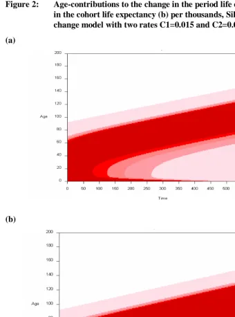
Figures 2ab show the Lexis surfaces of the age-specific contributions to the change in period and cohort life expectancy in a Siler mortality change model.
Figure 2: Age-contributions to the change in the period life expectancy (a) and in the cohort life expectancy (b) per thousands, Siler mortality change model with two rates C1=0.015 and C2=0.01
(a)
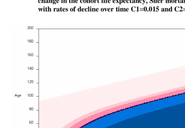
Figure 3 depicts the Lexis surface for the ratio of (i) the age-specific contributions to the change in period life expectancy over (ii) the corresponding age-specific contributions to the change in cohort life expectancy.
Figure 3: Ratio of age-specific contributions to the change in the period over change in the cohort life expectancy, Siler mortality change model with rates of decline over time C1=0.015 and C2=0.01
Figure 3 shows the steady increase over time in the age at which the ratio is 1. In the early years, the ratio is above 1 at most ages. That indicates that most ages make greater age-contributions to the period LE as infant mortality plays a larger role. At time 600, most of the ratios are below 1, showing that cohorts benefit more over a wide range of ages. However, at year 600 period LE is 116.8 and it is at advanced ages where most of the improvements in mortality are occurring. This increase in the age at which the ratio is one parallels the increase of life expectancies in Figure 1, with an accelerated pace at the beginning and a slower pace later.
+
+
=
+
)
,
(
)
,
(
)
,
(
)
,
(
)
,
0
(
)
,
0
(
, ,t
a
e
a
t
a
e
t
a
a
t
a
t
e
a
t
e
c p c p a c a pl
l
&
&
.Higher mortality in the past causes fewer cohort survivors to age a,
l
c(
a
,
t
)
, than in the corresponding period,l
p(
a
,
t
+
a
)
, implying numbers always above 1 for thismeasure of the past. Contrary to this is the ratio of remaining life expectancy, where cohort values are higher than period, indicating a ratio always below 1 for this measure of the future.
Figure 3 shows that at any given time the ratio increases with age. For younger ages it is below one, indicating that changes at those ages have more impact on cohort than period life expectancy. With mortality declining over time, young cohorts at time t will experience death rates at older ages lower than those experienced by older persons at time t, while differences in survivorship remain modest. Therefore, in equation (4) the ratio of period to cohort LE dominates the ratio of period to cohort survivorship. The inverse process occurs at older ages where the values of the ratio are above one. The cohorts that reach advanced ages at time t have experienced death rates at earlier ages greater than those seen in the period t, while the period to cohort LE ratio is modest.
5. Examining period and cohort mortality in Sweden
To assess age-specific contributions to period and cohort life expectancy in Sweden, we use data derived from the Human Mortality Database (2004). To calculate the age-specific contributions to cohort life expectancy for cohorts that are not extinct we have extrapolated future mortality. That was done using a continually declining mortality model, similar to that in equation (5), with a constant pace of decline of C=0.01. For example, if the last year with available data is 2002, then the age-specific death rates for that year,
µ
(a
,
2002
)
are the base values for the model. For age a and year t > 2002 the force of mortality is
( )
,
=
(
,
2002
)
−C(t−2002)e
a
t
a
µ
µ
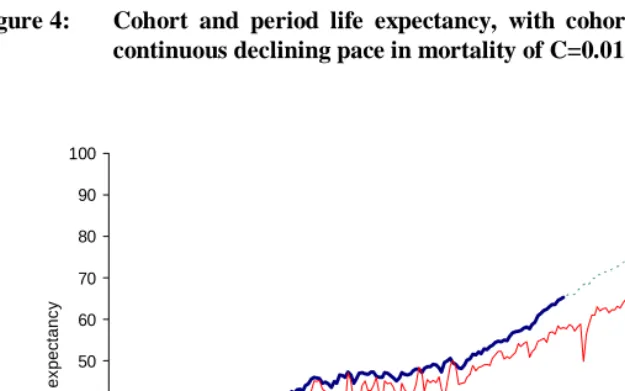
. (9)Figure 4 presents the period and cohort life expectancies in Sweden 1751-2002 with extrapolated cohort values for the years 1912 to 2002 using the death rates given by equation (9).
Figure 4: Cohort and period life expectancy, with cohorts completed with a continuous declining pace in mortality of C=0.01, Sweden
0 10 20 30 40 50 60 70 80 90 100
1751 1771 1791 1811 1831 1851 1871 1891 1911 1931 1951 1971 1991 Year
Li
fe
ex
pec
tanc
y
During the last years of the twentieth century the fluctuations observed in the period measure have largely disappeared. The estimated values of the cohort life expectancy, with the selected decline over time, correspond to a gap of around 7 years between the two life expectancies for 1911. Before 1900, however, that gap was much smaller and more erratic.
The gap observed between period and cohort life expectancies begins at the middle of the nineteenth century in Sweden. This is also the period of great improvement in infant mortality which contributes to the increase in both life expectancies, but more marked for the cohort measure. From about 1880 on, the pattern in Figure 4 resembles that in Figure 1.
Equations (6)-(8) show the relations between gaps and lags in a simple mortality model. These equations can be used for Sweden assuming that life expectancy moves linearly with a constant slope. This linear assumption has been shown to be realistic in developed countries over the last half of the 20th century (White, 2002). For Sweden, in 1911, the last year with full information on cohorts, the period and cohort life expectancies were 58.0 and 65.2 respectively. The gap between period and cohort life expectancies was thus 7.2 years. Calculating the derivative as the average of all annualized changes in period life expectancy from 1911 to each year from 1912 through 1950 we obtain an average slope of 0.30. Applying equation (6), a lag of 24 years is found. Comparing the cohort life expectancy of 65.3 in 1911 with 64.9, the period LE in year 1935, gives a discrepancy of only 0.4 years.
Period life expectancy in the industrialized world has followed a linear trend during the second half of the twentieth century so equation (6) should give a good approximation of the lags implied by the observed gaps (Goldstein and Wachter, 2005). For example, in 1950 cohort life expectancy was 79.5 years, with period life expectancy 8.4 years lower. For the year 1999, period life expectancy is 79.5, reaching the cohort value of 49 years earlier. With the slope of period life expectancy calculated as 0.18, equation (6) gives a lag of 46.7 years, which is 2.3 years below the actual lag of 49 years. However, the period life expectancy for 1997, the estimated year, was 79.3, giving an error in the lag of only 0.2 years.
Figure 5: Ratio of the period over the cohort age-contribution, Sweden 1900-2002. Cohorts completed with a pace of decline over time C=0.01
6. Conclusions
The disparity between period and cohort life expectancy can be measured at a given time or over the number of years it takes for period LE to attain the cohort level. For our continuously declining mortality model these two measures are linked by a simple relationship. For the industrialized world, where countries have experienced linear trends in life expectancy in the last half century, a similar though approximate relationship exists. While the cohort-period gap is fairly small and grows slowly over time, the lag is sizeable and grows much more rapidly.
To further analyze the dynamics of the two life expectancies we examine the age-specific contribution of changes in death rates to period and cohort life expectancy. Cohort life expectancy gains more from changes at younger ages, while the period measure gains more at older ages. The ratio of the contributions to period over cohort life expectancy can be seen as the product of two terms accounting for past and future changes in mortality. At the age when past mortality experience is balanced by future changes the ratio is one. As infant mortality falls to low levels improvements are concentrated at older ages, and the balancing age rises.
The present pattern of mortality change suggests widening cohort-period gaps and especially lags, as experience at more and more ages contributes more to cohort LE than to period LE.
7. Acknowledgments
References
Andreev, Evgueni M. 1982. “Method Komponent v Analize Prodoljitelnosty Zjizni.” [The Method of Components in the Analysis of Length of Life]. Vestnik Statistiki 9:42-47.
Andreev, Evgueni M., Vladimir Shkolnikov and Alexander Z. Begun. 2002. “Algorithm for Decomposition of Differences Between Aggregate Demographic Measures and its Application to Life Expectancies, Gini Coefficients, Health Expectancies, Parity-Progression Ratios and Total Fertility Rates.” Demographic Research 7:499-522.
Arriaga, Eduardo E. 1984. “Measuring and Explaining the Change in Life Expectancies.” Demography 21:83-96.
Bongaarts, John and Griffith Feeney. 2002. “How Long Do We Live?” Population and Development Review 28(1):13-29.
Bongaarts, John. 2005. “Long-Range Trends in Adult Mortality: Models and Projection Methods.” Demography 42(1):23-49.
Demetrius, Lloyd. 1979. “Relations Between Demographic Parameters.” Demography 16:329-338.
Gage, Timothy and Bennett Dyke. 1986. “Parameterizing Abridged Mortality Tables: The Siler Three-Component Hazard Model.” Human Biology 58(2):275-291. Goldman, Noreen and Graham Lord. 1986. “A New Look at Entropy and the
Lifetable.” Demography 23:275-282.
Goldstein, Joshua R. and Kenneth W. Wachter. 2005. “Gaps and Lags: Relationships Between Period and Cohort Life Expectancy.” Unpublished Manuscript, Princeton University and University of California, Berkeley.
Hill, Gerry. 1993. “The Entropy of the Survival Curve: An Alternative Measure.” Canadian Studies in Population 20:43-57.
Hokkert, Ralph. 1987. “Lifetable Transformations and Inequality Measures: Some Noteworthy Formal Relations.” Demography 24:615-622.
Keyfitz, Nathan. 1977. “What Difference Does it Make if Cancer Were Eradicated? An Examination of the Taeuber Paradox.” Demography 14:411-418.
---. 1985. Applied Mathematical Demography. 2nd ed. New York: Springer. Mitra, S. 1978. “A Short Note on the Taeuber Paradox.” Demography 15:621-623. Pollard, J. H. 1982. “The Expectation of Life and its Relationship to Mortality.”
Journal of the Institute of Actuaries 109:225-240.
---. 1988. “On the Decomposition of Changes in Expectation of Life and Differentials in Life Expectancy.” Demography 25:265-276.
Pressat, Roland. 1985. “Contribution des écarts de Mortalité par Age la Différence des Vies Moyennes.” Population 4-5:765-770.
Preston, Samuel, H., Patrick Heuveline and Michel Guillot. 2001. Demography: Measuring and Modeling Population Processes. Oxford: Blackwell Publishers.
Schoen, Robert and Vladimir Canudas-Romo. 2004. “Changing Mortality and Average Cohort Life Expectancy.” Paper presented at the workshop on Tempo Effects on Mortality, November 18-19, New York.
Schoen, Robert, Stefan H. Jonsson and Paula Tufis. 2004. “A Population with Continually Declining Mortality.” Working Paper 04-07, Population Research Institute, Pennsylvania State University, University Park, PA.
Siler, William. 1979. “A Competing-Risk Model for Animal Mortality.” Ecology 60(4):750-757.
United Nations. 1982. Levels and Trends of Mortality Since 1950, Study 74. New York: United Nations; Dept. of International Economic and Social Affairs.
Vaupel, James W. 1986. “How Change in Age-Specific Mortality Affects Life Expectancy.” Population Studies 40:147-157.
Vaupel, James W. and Vladimir Canudas-Romo. 2003. “Decomposing Change in Life Expectancy: A Bouquet of Formulas in Honor of Nathan Keyfitz's 90th Birthday.” Demography 40(2):201-216.
White, KM. 2002. “Longevity Advances in High-Income Countries 1955-96.” Population and Development Review 28(1):59-76.