of peer-reviewed research and commentary in the population sciences published by the Max Planck Institute for Demographic Research Konrad-Zuse Str. 1, D-18057 Rostock · GERMANY www.demographic-research.org
DEMOGRAPHIC RESEARCH
VOLUME 9, ARTICLE 9, PAGES 197-222
PUBLISHED 04 NOVEMBER 2003
www.demographic-research.org/Volumes/Vol9/9/
DOI: 10.4054/DemRes.2003.9.9
Descriptive Findings
Seasonal mortality in Denmark:
the role of sex and age
Roland Rau
Gabriele Doblhammer
1 Introduction 198
2 Data and Methods 199
3 Results 204
4 Discussion 211
5 Conclusion 214
6 Acknowledgements 214
Notes 214
References 216
Seasonal Mortality in Denmark:
The role of sex and age
Roland Rau1
Gabriele Doblhammer2
Abstract
Our paper addresses two questions on seasonal mortality: How do women and men differ with respect to seasonal fluctuations in mortality? How does seasonality in death change with age? The analysis is based on a sample of all Danes aged 50 and older on 1 April 1968 who were followed for 30 years.
In contrast to previous studies we found remarkable differences between women and men in their seasonal mortality patterns. Men showed larger seasonal fluctuations than women indicating a higher susceptibility to environmental stressful periods.
We found that seasonality increases with age. However, we discovered again a sex difference: women’s seasonality starts increasing at later ages than men’s.
1Max Planck Institute for Demographic Research, Konrad Zuse Str. 1, 18057 Rostock, Germany. E-mail:
2Max Planck Institute for Demographic Research, Konrad Zuse Str. 1, 18057 Rostock, Germany. E-mail:
1
Introduction
“Death strikes from every side, but not at random” (March, 1912, p. 505). While an in-dividual death may not be predicted, it is possible to make a probabilistic forecast about the timing of death. In Western countries, one is most likely to die during the first few months of the year. During summer, on the contrary, mortality is lowest (Aubenque et al., 1979; Feinstein, 2002; Hernández and García-Moro, 1987; Kunst et al., 1990; Lerchl, 1998; Lyster, 1972; Mackenbach et al., 1992). These fluctuations “are one of the ‘deep structures’ that identify the main environmental and cultural factors that form a given population” (Shaw, 1996, p. 100). Although climate shapes the basic seasonal pattern of mortality, one cannot necessarily equate colder climate with larger monthly oscillations. Indeed, Canada, Russia and the Scandinavian countries show a lower percentage of ex-cess deaths during winter than, for example, the UK and many Mediterranean countries (Grut, 1987; McKee, 1989). It has been estimated for the late 1970s that about half a million deaths per year in North America, the USSR, and Europe were cold-related (Grut, 1987). It is argued that these deaths are mainly an outcome of exposure to outdoor and indoor cold; people living in rather severe climatic zones protect themselves better against both kinds of hazards (Donaldson et al., 1998; Donaldson and Keatinge, 2002; Donaldson et al., 1998; Eurowinter Group, 1997, 2000; Keatinge, 1986; Keatinge et al., 1989).
point into the direction that it was caused by the “between wars” cohorts of women who have the highest mortality rates for lung cancer and chronic obstructive pulmonary disease anywhere in Europe. These causes of death are usually associated with the high smoking prevalence of those cohorts (Jacobsen et al., 2002; Juel, 2000). [Note 2]
Instead of examining the trend over time, we analyzed in this pilot study the factors sex and age. They usually received little attention in previous studies, despite their paramount influences on mortality (Rogers et al., 1995, p. 7–8). A usual assumption among demog-raphers asserts that mortality measures the current conditions of the ecological and social environment (Robine, 2001). According to that assessment, women and men vary in their susceptibility towards environmental hazards as reflected by the lower female age-specific mortality-rates throughout the life-course. Consequently, we were puzzled by the results of several studies on seasonality that included the factor sex. They typically found no significant differences between women and men in seasonality in all-cause mortality (Eu-rowinter Group, 1997; Gemmell et al., 2000; Nakai et al., 1999; Yan, 2000).
The factor age has been analyzed in more detail than sex. However, the basis of the data implied some problems in previous studies. Sometimes no age distinction was made at all (Aubenque et al., 1979; Barrett, 1990; Rosenwaike, 1966; Trudeau, 1997). In other studies the highest included age or the beginning of the last, open-ended, age category was chosen at an age after which most deaths in a population occur (Bull and Morton, 1978; Crombie et al., 1995; Donaldson et al., 1998; Eurowinter Group, 1997, 2000; Human Life-Table Database, 2003; Huynen et al., 2001; Keatinge et al., 1989; Mc-Kee et al., 1998; Underwood, 1991). Thus, results from these studies may simplify or blur the relationship between age and seasonal fluctuations in mortality. Some studies an-alyzed heat-related mortality up into very advanced ages (Mackenbach et al., 1997; Nakai et al., 1999), but only a few investigated overall seasonal mortality in these age-groups (Feinstein, 2002; McDowall, 1981; Näyhä, 1980). [Note 3] The general trend in those studies asserts an increase of seasonality with age. This fits our framework of decreasing resistance towards environmental hazards with age.
2
Data and Methods
other countries in respect to the amount of possibly preventable deaths:
EWD=D−
µ
12×DJUL+DAUG+DSEP 3
(1)
EWD represents the number of excess winter deaths,Dis the number of all deaths during the follow-up andDJUL,DAUG,DSEPrepresent the number of deaths during July, August, and September, respectively. The proportion of winter excess deaths is obtained by computing EWD/D.
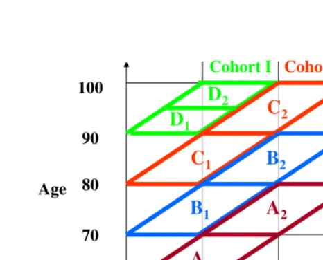
Figure 1: Cohort Distinction in a Lexis-Diagram
Our main objective was to analyze the changing risks of dying in different months of the year. We created a data-set that contains a person as many times as he/she has lived in months between April 1968 and March 1998. When using the whole Danish population at ages 50+ this procedure would lead to a huge data-set. We therefore opted to draw a random-sample of each cohort and sex. The final data-set included 46,293 individuals (≈
and sex.
Figure 2: Graphical Outline of Data-Set for Analysis by Age
We further divided the population by using four ten-year birth cohorts: the oldest cohort (Cohort I)was born between April 1878 and March 1888. In April 1968 they were aged between 80 and 89 years and 11 months. We followed them until they reached a maximum age of 99 years and 11 months (March 1978 to March 1988). The second
cohort(birth dates between April 1888 and March 1898) is aged 70 to 79 years and 11
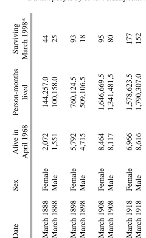
months in 1968 and is followed to age 99 years and 11 months (time period March 1988 - March 1998).The third cohort(born April 1898 — March 1908) is aged 60 to 69 years and 11 months at baseline. At the end of the follow-up (March 1998) they have reached ages 90 to 99 and 11 months.The fourth cohort(born April 1908 — March 1918) is aged 50 to 59 and 11 months at baseline and reaches maximum ages of 80 to 89 and 11 months in March 1998. Please see Figure 1 for a graphical description of this classification. The exact numbers of individuals in each cohort by birth date, sex, and survival status are given in Table 1. We controlled for different length of month by standardizing all records to a weight of 30 days.
goal was that every member of a specific cohort should theoretically be able to reach each analyzed age. For example, people inCohort IIIwho were 60 years old in the beginning of the follow-up could attain a maximum of 90 years. Analogously, people in the same cohort aged 69 years in 1968 have no possibility to be exposed to the risk of dying at age 65 anymore. Therefore, we transformed the cohorts into parallelograms as follows (see Figure 2):
In each of the cohorts we constructed two age groups. The oldest cohort was followed from age 90 (time period April 1968 to April 1978) until they reached the age 94 years and 11 months (Fig. 2,D1). Within the same birth cohort we compared this age group with the 5-year age group that reached age 95 between April 1973 and April 1978 and attained a maximum age of 99 years and 11 months between March 1978 and March 1988 (D2). In the second cohort the first age group consists of all those who were aged 80 in the time period April 1968 to April 1973 and reached a maximum age of 89 years and 11 months between March 1978 and March 1988 (C1). The second age group in Cohort II comprises ages 90 (time period April 1978 to April 1988) to 99 years and 11 months (time period March 1988 to March 1998) (C2). The first age group in the third cohort consists of ages 70 to 79 years and 11 months (B1), the second of ages 80 to 89 years
and 11 months (B2). In the youngest cohort, the first age group comprises ages 60 to 69
years and 11 months (A1); the second age group, ages 70 to 79 years, 11 months (A2). The time periods for the respective age groups in the two youngest cohorts are the same as those specified in Cohort II.
We analyzed the mortality of our subjects using a logistic regression model. [Note 4] Following Allison (1995), the effects of the covariates are modeled by using Equation 2:
log
µ Pit
1−Pit 
=αt+ 11
∑
m=1βmxi,m+δPeriodvi,t+γAgewi,t (2)
Table 1: Sample Population of follow-up from 1968 until 1998 of elderly
Danish people by cohort classification, sex, and survival status
Hewitt’s test (Hewitt et al., 1971) was employed to investigate whether the relative risks of dying follow a seasonal pattern. This test gives ranks to each month. The value “12” is assigned to the month with the highest relative risk, and “1” to the month with the lowest relative risk. Keeping the original order of the months (January, February, ..., December), the test statistic is the maximum rank-sum of six consecutive months. Thus, this method assumes that the year is split into two 6-months-periods with a relatively high risk to experience the event in one half and a relatively low risk during the other half. Simulated significance levels (Hewitt et al., 1971) were applied for Hewitt’s test if exact values were not available (Walter, 1980).
3
Results
Monthly standardized death counts:
⇒Denmark displays the typical Western pattern.
Figure 3 shows the monthly distribution of the 1,171,535 deaths of the whole data-set in percent after standardizing each month to thirty days. The bars indicate a season-ally changing pattern peaking in January (number of standardized deaths: 106,037) and reaching a minimum in August (88,395 standardized deaths). According to our definition 78,375 deaths during our observation period of 30 years can be attributed to winter excess mortality or more than 2,600 deaths each year. This equals a proportion of 6.69 percent of all deaths.
Monthly odds ratios for the four cohorts:
⇒Seasonal fluctuations are larger in the older cohorts.
Figure 3: Distribution of Monthly Mortality in Percent after Standardizing Length
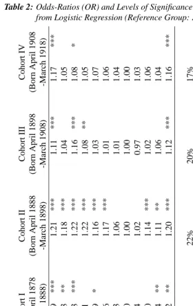
Table 2: Odds-Ratios (OR) and Levels of Significance for Month of Death
from Logistic Regression (Reference Group: August)
Sex-specific odds ratios by season for the four cohorts:
⇒Men experience larger seasonal fluctuations in mortality than women.
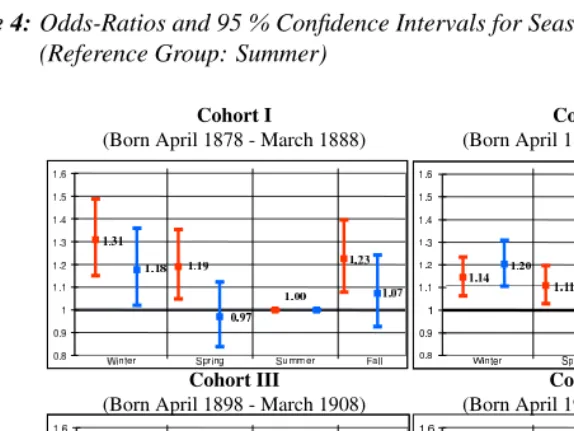
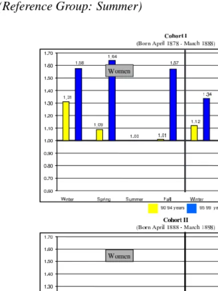
Figure 4 gives the result of a similar estimation as Table 2 with two exceptions: First, we conducted separate analyzes for women and men. Second, months have been summa-rized to seasons (Winter: January, February, March;Spring: April, May, June;Summer: July, August September;Fall: October, November, December) to clarify trends.
Figure 4: Odds-Ratios and 95 % Confidence Intervals for Seasonal Mortality by Sex
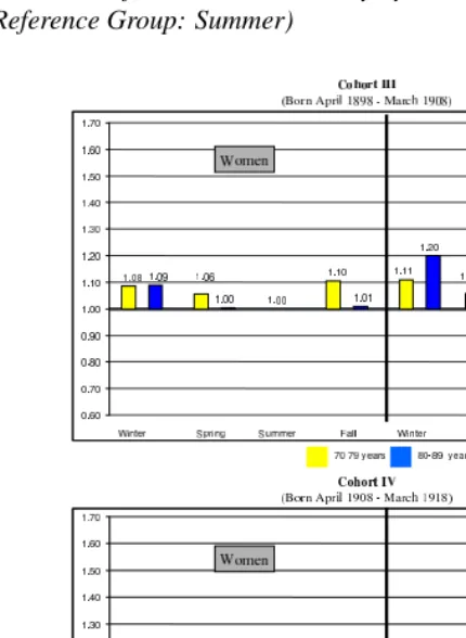
Figure 5: Odds-Ratios for Seasonal Mortality by Sex and Age-Group Part I
Figure 6: Odds-Ratios for Seasonal Mortality by Sex and Age-Group Part II
The youngest cohort (Cohort IV: ages 50/59 to ages 80/89, time period 1968 to 1998) displays virtually no difference between the sexes. With odds-ratios of 1.08 for women and 1.07 for men, the mortality risk is highest for both sexes in winter. Cohort III (ages 60/69 to ages 90/99, time period 1968 to 1998), which is on average 10 years older than Cohort IV, shows a similar pattern with a peak in winter and a trough in summer for both sexes. However, the relative mortality risk is remarkably higher for men than for women (OR winter: 1.14 vs 1.08; OR spring: 1.07 vs. 1.03; OR fall: 1.10 vs 1.06). Since both cohorts cover the same time period the increase in the seasonality must be due to differ-ences in age.
In Cohort II (ages 70/79 to age 99, time period 1968 to 1988/1989), men face excess mortality of 20 percent in winter and 21 percent in spring, women’s excess mortality is 1.14 and 1.11, respectively. The oldest people (Cohort I: ages 80/89 to age 99, time period 1968 to 1978/1988) are reversing the trend. Men’s seasonal fluctuations are smaller than women’s and their trough changed from summer to spring (OR spring: 0.97). Women in that cohort faced higher relative risks during each season than in any other cohort, reach-ing a maximum in winter with a relative risk of 31 percent in winter compared to summer. Since the oldest cohort only covers the time period 1968/1973 to 1978/ 1983 (opposed to the other cohorts covering 1968/1978 to 1988/98), we cannot distinguish whether the particular pattern in this cohort is due to age effects or period effects.
Sex and age-specific odds ratios by season for the four cohorts:
⇒Seasonal fluctuations in mortality start increasing at later ages for women than for men.
Figures 5 and 6 show the effect of age on the seasonality in mortality. Men, generally speaking, exhibit an increase of seasonal mortality fluctuations with age. In the youngest cohort the relative mortality risk for septagenarians compared to 60-69 year olds increased by 1 percentage point in spring, 5 percentage points in fall, and by 6 percentage points in winter. The increase in fluctuations further intensifies in the oldest cohort. In addition, we observe an intermediary peak in mortality during summer among the oldest men.
1.01 to 1.57 in fall. Contrary to men, we do not observe a summer peak among women.
4
Discussion
Before discussing the results, it is useful to briefly point out the advantages of the study. Some of the potential shortcomings will be discussed at the end of this section. The design of our data-set makes our analysis unique. The major drawback of previous longitudinal studies was the non-availability of the exact risk-set. Either researchers used deaths counts (e.g. Gemmell et al., 2000; Trudeau, 1997) or interpolated data to obtain the specific population at risk (e.g. Mackenbach et al., 1992; Marshall et al., 1988). To our knowledge, only one previous longitudinal study used exact exposures and occurrences of events (van Rossum et al., 2001). However, our analysis has the advantage that it is based on a sample of the whole population and is, therefore, not restricted to one occupation (civil servants) and one sex (men) (van Rossum et al., 2001).
We found that mortality in Denmark follows the well-known seasonal pattern of coun-tries in the Northern Hemisphere. Denmark is experiencing 2,612 winter excess deaths annually, which corresponds to a proportion of 6.69 percent of all deaths. Denmark is on level terms with the US in 1978 (Grut, 1987) and fares better compared to some other European countries like Ireland (14.6%) and Portugal (13.7%) during the period 1976– 83. However, a comparison (McKee, 1989) with its neighboring countries in the Baltic like West Germany (5.4%), Sweden (5.4%), Norway (3.9%), and Finland (3.8%) during 1976–84 lets us conclude that further progress can be made in Denmark in reducing the annual cold-related death toll.
It is open to discussion how large the effect of saving lives in winter on mortality in general actually is. Two extreme opinions are imaginable. The true effect will lie some-where in between: either one assumes that the subject is in a frail condition and would have died anyway relatively soon. The other assumption would be that the individual does not differ in his/her robustness from the rest of the population. Saving a life in the latter case would be “perfect repair” in terms of reliability engineering. Further analysis on the actual causes of death could shed some light on this question. If accidents and infectious diseases dominated the seasonal fluctuations, the overall effect could rather tend towards the “perfect repair extreme”. Contrastingly, if chronic diseases mainly shaped the sea-sonal pattern, the effect on reducing overall mortality would either be relatively small or it would require more efforts in medicine, public health and general living improvements to obtain the same effect as in the other case where relatively inexpensive interventions like vaccinations may result in remarkable improvements.
an increase with age in the amplitude of the monthly mortality risks. But not only the heights of the fluctuations were increasing. Also the seasonal pattern changed. We can make a broad distinction between the relatively older cohorts (Cohorts I and II) on the one hand and the younger cohorts (Cohorts III and IV) on the other hand. In the older cohorts, the trough is restricted to the three warmest months (July-September). Throughout the remainder of the year, excess mortality is relatively high. The younger group, conversely, shows a different pattern. The trough ranges approximately from spring until early fall. Peaks in mortality can only be found in the coldest months. This result may indicate a change in the sensitivity towards environmental hazards with age: in the two younger co-horts, only the extreme cold weather proved to be dangerous for the Danish. If we look, though, at the two older cohorts, we can see that anything else but summer climate seems to be perilous for survival for women.
The intermediary summer peak for men suggests that the oldest men are affected by extreme climatic conditions in general: cold weather in winter as well as hot spells during summer. We suspect that this changing pattern has been missed by previous studies either because of the limited age-range they investigated or by an underrepresentation of people at very advanced ages.
The slight mortality dip in all cohorts in February suggests a similar explanation as hypothesized for historical English populations by Oeppen (Oeppen, 2003): while people dying in January rather die of immediate causes of the cold climate, deaths in March are due to the accumulation of detrimental effects during the cold season.
Our data helps to explain the surprising result of previous studies which found no sex differences in relation to seasonal mortality (Eurowinter Group, 1997; Gemmell et al., 2000; Nakai et al., 1999; Yan, 2000): we find the same result — but only for the youngest cohort (Cohort IV). In the remaining three cohorts women and men differ to a large extent. We can therefore claim that the limited age-range used in previous studies is too narrow to conclude that the susceptibility towards cold-related hazards does not differ between women and men.
the oldest displayed the highest death rates during heat spells. However, Mackenbach and his colleagues (Mackenbach et al., 1997) found contradictory evidence: women’s excess mortality during hot periods is higher than men’s. Additionally, age “does not appear to be consistently related to excess mortality at high outside temperatures” (Mackenbach et al., 1997, p. 1298). Due to these opposing views in the literature, we suppose that our finding may be the outcome of a compositional effect, too (third possible explanation): as the frail tend to die earlier, the male survivors in the oldest cohort (Cohort I) are a selected subsample of their initial birth cohort being more robust on average.
Among men, seasonal mortality fluctuations increase with age. We suggest two expla-nations for the stationary or even decreasing trend for women in the two younger cohorts: either women actually have increasing seasonal fluctuations in mortality but this trend is offset by beneficial period-effects. However, this explanation seems to be less likely as it implies that some secular events had positive consequences for women in those age-ranges but neither at later ages nor for men. We rather support the opposing idea that the aging process in the younger observed age-groups does not affect the relatively strong resistance of women towards changing environmental hazards. At later ages women also face an increasing susceptibility with age. Our interpretation therefore is that women as well as men show larger seasonal fluctuations in mortality as they age. The main differences are that women’s susceptibility starts at later ages and is restricted to cold temperatures. Men, on the contrary, show increases with age already at younger ages. In the oldest observed age-categories, men have become not only susceptible to cold outside temperatures but to any unfavourable climatic conditions (e.g. summer heat).
5
Conclusion
This study analyzed seasonal mortality in Denmark which is relatively high compared to its neighboring countries. We have shown that the previous assessment that women and men do not differ with respect to seasonal fluctuations in mortality tends to be an oversim-plification. Men seem to be more susceptible to hazardous environmental conditions than women. This is what one could expect from the generally lower female mortality rates throughout the life-course. We found evidence that seasonality increases with age. How-ever, the pattern varies between women and men. Women’s seasonal fluctuations start increasing at later ages than men’s. Compared to women, men seem to be susceptible not only to cold weather but also to extreme hot climatic conditions.
Tackling seasonal mortality will gain further relevance for public health researchers from two directions. First, the chances to survive into ages where seasonal fluctuations in mortality reach remarkable levels are increasing (Kannisto et al., 1994; Vaupel, 1997). Secondly, the vast amount of literature on risk factors and the smaller fluctuations in regions with colder climate let us conclude that the annual amount of excess mortality may be reducible by preventive health and safety measures (Trudeau, 1997).
6
Acknowledgements
The authors would like to thank Francesco C. Billari for his valuable technical comments and two anonymous referees; the readability of the paper benefitted from the advice of Maggie Kulik and Uta Ziegler.
Notes
1. Oeppen and Vaupel (2002) calculated for women an increase of 0.243 years of age for every calendar year passed.
2. It has been seriously suggested but also heavily contested that the reason for the high smoking prevalence of the “between wars” generation of Danish women is caused by the bad role model effect of the smoking Queen Margrethe II (Jacobsen et al., 2001; Kesteloot, 2001; Madsen, 2001).
References
Allison, P. D. (1982). Discrete-time methods for the analysis of event histories. Sociolog-ical Methodology 13, 61–98.
Allison, P. D. (1995). Survival Analysis Using the SAS System. Cary, NC: SAS Institute Inc.
Aubenque, M., P. Damiani, and H. Massé (1979). Variations saisonnières et séries chronologiques des causes de décès en France de 1900 à 1972. Cahiers de Sociolo-gie et de Démographie Médicales 19, 17–22.
Aylin, P., S. Morris, J. Wakefield, A. Grossinho, L. Jarup, and P. Elliott (2001). Temper-ature, housing, deprivation and their relationship to excess winter mortality in Great Britain, 1986–1996. International Journal of Epidemiology 30, 1100–1108.
Barrett, R. E. (1990). Seasonality in vital processes in a traditional Chinese population. Modern China 16, 190–225.
Bull, G. and J. Morton (1978). Environment, temperature and death rates. Age and Ageing 7, 210–224.
Chenet, L., M. Osler, M. McKee, and A. Krasnik (1996). Changing life expectancy in the 1980s: why was Denmark different from Sweden? Journal of Epidemiology and Community Health 50, 404–407.
Clinch, J. P. and J. D. Healy (2000). Housing standards and excess winter mortality. Journal of Epidemiology and Community Health 54, 719–720.
Crombie, D., D. Fleming, K. Cross, and R. Lancashire (1995). Concurrence of monthly variation of mortality related to underlying cause in europe. Journal of Epidemiology and Community Health 49, 373–378.
Dolley, M. (1994). Denmark tries to raise life expectancy. British Medical Journal 308, 737–738.
Donaldson, G., S. Ermakov, Y. Komarov, and W. Keatinge (1998). Cold related mortali-ties and protection against cold in Yakutsk, eastern Siberia: observation and interview study. British Medical Journal 317, 978–982.
Donaldson, G., V. Tchernjavskii, S. Ermakov, K. Bucher, and W. Keatinge (1998). Winter mortality and cold stress in Yekaterinburg, Russia: interview study. British Medical Journal 316, 514–518.
Eurowinter Group (1997). Cold exposure and winter mortality from ischaemic heart disease, cerebrovascular disease, respiratory disease, and all causes in warm and cold regions of Europe. Lancet 349, 1341–1346.
Eurowinter Group (2000). Winter mortality in relation to climate. International Journal of Circumpolar Health 59, 154–159.
Feinstein, C. A. (2002). Seasonality of deaths in the U.S. by age and cause. Demographic Research 6, 469–486.
Gemmell, I., P. McLoone, F. Boddy, G. J. Dickinson, and G. Watt (2000). Seasonal variation in mortality in Scotland. International Journal of Epidemiology 29, 274–279.
Greenberg, J. H., J. Bromberg, C. Reed, T. L. Gustafson, and R. A. Beauchamp (1983). The epidemiology of heat-related deaths, Texas—1950, 1970–79, and 1980. American Journal of Public Health 73, 805–807.
Grut, M. (1987). Cold-related death in some developed countries. The Lancet (8526), 212. 24 January 1987.
Hernández, M. and C. García-Moro (1986–1987). Seasonal distribution of mortality in Barcelona (1983-1985). Antropol. Port. 4–5, 211–223.
Hewitt, D., J. Milner, A. Csima, and A. Pakula (1971). On Edwards’ criterion of seasonal-ity and a non-parametric alternative. British Journal of Preventive Social Medicine 25, 174–176.
Human Life-Table Database (2003, April). Data by country: Denmark.
Con-tributions from Väinö Kannisto and Danmarks Statistik, accessible online at:
http://www.lifetable.de.
Huynen, M. M., P. Martens, D. Schram, M. P. Weijenberg, and A. E. Kunst (2001). The impact of heat waves and cold spells on mortality rates in the Dutch population. Envi-ronmental Health Perspectives 109, 463–470.
Jacobsen, R., N. Keiding, and E. Lynge (2002). Long term mortality trends behind low life expectancy of Danish women. Journal of Epidemiology and Community Health 56, 205–208.
Juel, K. (2000). Increased mortality among Danish women: population based register study. British Medical Journal 321, 349–350.
Kannisto, V., J. Lauritsen, A. R. Thatcher, and J. W. Vaupel (1994). Reductions in mortal-ity at advanced ages: Several decades of evidence from 27 countries. Population and Development Review 20, 793–810.
Keatinge, W. (1986). Seasonal mortality among elderly people with unrestricted home heating. British Medical Journal 293, 732–733.
Keatinge, W., S. Coleshaw, and J. Holmes (1989). Changes in seasonal mortality with improvements in home heating in England and Wales from 1964 to 1984. International Journal of Biometeorology 33, 71–76.
Keatinge, W. and G. Donaldson (2001). Warm housing is not enough (letters). British Medical Journal 323, 166.
Kesteloot, H. (2001). Queen Margrethe ii and mortality in Danish women. The Lanceet 357, 871–872.
Kunst, A., C. Looman, and J. Mackenbach (1990). The decline in winter excess mortality in the Netherlands. International Journal of Epidemiology 20, 971–977.
Lawlor, D., R. Maxwell, and B. Wheeler (2002). Rurality, deprivation, and excess winter mortality: an ecological study. Journal of Epidemiology and Community Health 56, 373–374.
Lawlor, D. A., D. Harvey, and H. G. Dews (2000a). Investigation of the association between excess winter mortality and socio-economic deprivation. Journal of Public Health Medicine 22, 176–181.
Lawlor, D. A., D. Harvey, and H. G. Dews (2000b). Investigation of the association between excess winter mortality and socio-economic deprivation. Journal of Public Health Medicine 22, 176–181.
Lerchl, A. (1998). Changes in the seasonality of mortality in germany from 1946 to 1995: the role of temperature. International Journal of Biometeorology 42, 84–88.
Mackenbach, J., A. Kunst, and C. Looman (1992). Seasonal variation in mortality in The Netherlands. Journal of Epidemiology and Community Health 46, 261–265.
Mackenbach, J. P., V. Borst, and J. M. Schols (1997). Heat-related mortality among nursing-home patients. The Lancet 349, 1297–1298.
Madrigal, L. (1994). Mortality seasonality in Escazú, Costa Rica, 1851–1921. Human Biology 66, 433–452.
Madsen, S. (2001). Queen Margrethe ii and mortality in Danish women. The Lancet 358, 75.
March, L. (1912). Some researches concerning the factors of mortality. Journal of the Royal Statistical Society 75, 505–538.
Marcuzzi, G. and M. Tasso (1992). Seasonality of death in the period 1889-1988 in the Val di Scalve (Bergamo Pre-Alps, Lombardia, Italy). Human Biology 64, 215–222.
Marshall, R. J., R. Scragg, and P. Bourke (1988). An analysis of the seasonal variation of coronary heart disease and respiratory disease mortality in New Zealand. International Journal of Epidemiology 17, 325–331.
McDowall, M. (1981). Long term trends in seasonal mortality. Population Trends 26, 16–19.
McKee, C. M. (1989). Deaths in winter: Can Britain learn from Europe? European Journal of Epidemiology 5(2), 178–82.
McKee, M., C. Sanderson, L. Chenet, S. Vassin, and V. Shkolnikov (1998). Seasonal variation in mortality in Moscow. Journal of Public Health Medicine 20, 268–274.
Nakai, S., T. Itoh, and T. Morimoto (1999). Deaths from heat-stroke in Japan: 1968–1994. International Journal of Biometeorology 43, 124–127.
Näyhä, S. (1980). Short and medium term variations in mortality in Finland. Ph. D. thesis, Department of Public Health Service, University of Oulu, Finland.
Oeppen, J. (2003). personal communications. Cambridge Group for the History of Pop-ulation and Social Structure, Cambridge, UK.
Olsen, N. D. (2001). Prescribing warmer, healthier homes (Editorial). British Medical Journal 322, 748–749.
Robine, J.-M. (2001). A new biodemographic model to explain the trajectory of mortality. Experimental Gerontology 36, 899–914.
Robine, J.-M. and J. Vaupel (2001). Supercentenarians: slower ageing individuals or senile elderly? Experimental Gerontology 36, 915–930.
Rogers, R. G., R. A. Hummer, and C. B. Nam (1995). Living and Dying in the USA. Be-havioral, Health and Social Differentials of Adult Mortality. San Diege, CA: Academic Press.
Rosenwaike, I. (1966). Seasonal variation of deaths in the United States, 1951–1960. Journal of the American Statistical Association 61, 706–719.
Sakamoto-Momiyama, M. (1978). Changes in the seasonality of human mortality: A medico-geographical study. Social Science and Medicine 12, 29–42.
Shah, S. and J. Peacock (1999). Deprivation and excess winter mortality. Journal of Epidemiology and Community Health 53, 499–502.
Shaw, B. D. (1996). Seasons of Death: Aspects of Mortality in Imperial Rome. Journal of Roman Studies 86, 100–138.
Trudeau, R. (1997). Monthly and daily patterns of death. Health Reports (Statistics Canada) 9, 43–50.
Underwood, J. H. (1991). Seasonality of vital events in a Pacific island population. Social Biology 38, 113–126.
van Rossum, C. T., M. J. Shipley, H. Hemingway, G. D. E., J. P. Mackenbach, and M. J. Marmot (2001). Seasonal variation in cause-specific mortality: Are there high-risk groups? 25-year follow-up of civil servants from the first Whitehall study. International Journal of Epidemiology 30, 1109–1116.
Vaupel, J. W. (1997). The remarkable improvements in survival at older ages. Philosophi-cal Transactions of the Royal Society of London: BiologiPhilosophi-cal Sciences 352, 1799–1804.
Vaupel, J. W. and V. Canudas Romo (2002). Decomposing demographic change into direct vs. compositional components. Demographic Research 7, 1–14.
Wilkinson, P., M. Landon, B. Armstrong, S. Stevenson, S. Pattenden, M. McKee, and T. Fletcher (2001). Cold comfort. The social and environmental determinants of excess winter death in England, 1986–96. Bristol, UK: Policy Press.
Woodward, M. (1999). Epidemiology. Study Design and Data Analysis. Boca Raton, FL: Chapman and Hall / CRC.
A
Appendix
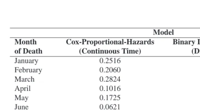
Table 1: Cox-Proportional-Hazards Model and Binary Logistic Regression yield
the same results in practice. An example from estimating the effect of current month on the chance of dying for Cohort I.
Model
Month Cox-Proportional-Hazards Binary Logistic Regression of Death (Continuous Time) (Discrete Time)
January 0.2516 0.2517
February 0.2060 0.2070
March 0.2824 0.2867
April 0.1016 0.1005
May 0.1725 0.1725
June 0.0621 0.0607
July 0.0335 0.0332
August Reference Group Reference Group
September 0.0421 0.0429
October 0.0977 0.0966
November 0.2144 0.2156