Distributed Support Vector Machine Learning

(1)

University of New Orleans University of New Orleans

ScholarWorks@UNO

University of New Orleans Theses and

Dissertations Dissertations and Theses

8-7-2008

Distributed Support Vector Machine Learning

Kenneth C. Armond Jr. University of New Orleans

Follow this and additional works at: https://scholarworks.uno.edu/td

Recommended Citation Recommended Citation

Armond, Kenneth C. Jr., "Distributed Support Vector Machine Learning" (2008). University of New Orleans Theses and Dissertations. 711.

https://scholarworks.uno.edu/td/711

This Thesis is protected by copyright and/or related rights. It has been brought to you by ScholarWorks@UNO with permission from the rights-holder(s). You are free to use this Thesis in any way that is permitted by the copyright and related rights legislation that applies to your use. For other uses you need to obtain permission from the rights-holder(s) directly, unless additional rights are indicated by a Creative Commons license in the record and/or on the work itself.

(2)

Distributed Support Vector Machine Learning

A Thesis

Submitted to the Graduate Faculty of the University of New Orleans in partial fulfillment of the requirements for the degree of

Master of Science in

Computer Science Bioinformatics

by

Kenneth C. Armond Jr.

B.S. Texas A&M University, 2003

(3)

Acknowledgment

I would like to thank my advisor, Dr. Stephen Winters-Hilt. He has helped me

tremendously to understand the importance of academic research. He gave me the enthusiasm

needed to begin research in the field of Bioinformatics, which I previously did not know

anything about. I aspire to keep this enthusiasm in future endeavors, as he has after years of

research. His intelligence and accomplishments make him an excellent mentor yet he still knows

how to balance work and fun.

I would like to thank Sam Merat who was my student mentor and we worked together on

the early SVM Java code that eventually led to further work on the different chunking methods

described here. His knowledge was integral to helping me understand the SVM algorithm.

I would like to thank Carl Baribault who was always happy and willing to answer the many

questions I had. His collaboration on the Support Vector Reduction method was very helpful. I

have gained much insight on a variety of subjects from talking with him.

I would also like to think the other members of the Bioinformatics group for their help and

support.

Finally, I would like to express my deep gratitude to my wife, Stephanie, and my son,

Linus. Their encouragement and unconditional support have made getting this degree much

(4)

List of Figures

Figure 3.1 SMO Support Vector Reduction ...21

Figure 3.2 Multi-threaded Chunking Support Vector Reduction ...22

Figure 3.3 Sequential Chunking Support Vector Reduction ...23

Figure 4.1 Sequential Chunking % Parameters ...29

(6)

List of Tables

Table 2.1 Multi-threaded chunking, various datasets, Absdiff kernel...12

Table 2.2 Multi-threaded chunking, various datasets, Sentropic kernel...13

Table 2.3 Multi-threaded chunking, various datasets, Gaussian kernel ...13

Table 2.4 Sequential chunking, various datasets, Absdiff kernel ...14

Table 2.5 Sequential chunking, various datasets, Sentropic kernel...14

Table 2.6 Sequential chunking, various datasets, Gaussian kernel...15

Table 2.7 Sequential chunking, 9GC9CG_9AT9TA dataset, Absdiff kernel...15

Table 2.8 Sequential chunking, 9GC9CG_9AT9TA dataset, Sentropic kernel ...16

Table 2.9 Sequential chunking, 9GC9CG_9AT9TA dataset, Gaussian kernel ...16

Table 2.10 Multi-threaded chunking, 9GC9CG_9AT9TA dataset, Absdiff kernel ...17

Table 2.11 Multi-threaded chunking, 9GC9CG_9AT9TA dataset, Sentropic kernel ...17

Table 2.12 Multi-threaded chunking, 9GC9CG_9AT9TA dataset, Gaussian kernel ...18

(7)

List of Illustrations

(8)

Abstract

Support Vector Machines (SVMs) are used for a growing number of applications. A

fundamental constraint on SVM learning is the management of the training set. This is because

the order of computations goes as the square of the size of the training set. Typically, training

sets of 1000 (500 positives and 500 negatives, for example) can be managed on a PC without

hard-drive thrashing. Training sets of 10,000 however, simply cannot be managed with PC-based

resources. For this reason most SVM implementations must contend with some kind of chunking

process to train parts of the data at a time (10 chunks of 1000, for example, to learn the 10,000).

Sequential and multi-threaded chunking methods provide a way to run the SVM on large datasets

while retaining accuracy. The multi-threaded distributed SVM described in this thesis is

implemented using Java RMI, and has been developed to run on a network of

multi-core/multi-processor computers.

Keywords

Distributed

Parallel

SVM

Support Vector Machine

Machine Learning

SMO

(9)

Chapter 1. Introduction

SVMs are becoming more popular since researchers and engineers find it to be a better,

more robust replacement for older learning methods such as neural networks. Another attractive

aspect of SVMs is that they do not require much manual parameter manipulation which makes

their use much easier. Neural networks are a good example of an outdated learning method that

requires a decent amount of expertise in order to get the training parameters properly set for each

different dataset. Many areas of study such as text categorization, face recognition, handwriting

recognition, pedestrian detection, and DNA hairpin classification are increasingly using SVMs as

their main classification method.

The main problem with current day SVMs is that they cannot process large datasets in a

timely manner. This problem is compounded further when multiple SVM training rounds are

needed as with SVM clustering methods being developed by the Winters-Hilt Group (but not

discussed further here). Chunking the training set into smaller datasets provides a solution to this

problem. Sequential chunking runs the SVM on the first chunk and then sends the support

feature vectors (SVs) and sometimes some non-SVs to be added into the training data for the

next chunk. This continues until all chunks have been run. What is not as commonly discussed

are multi-threaded chunk processing methods. In part, this may be because of the many subtleties

that have been encountered in these efforts and this is a major focus of this thesis.

Multi-threaded chunking breaks the training dataset into smaller chunks to be trained separately. When

all chunks have been trained, SVs and sometimes some non-SVs are brought together and

re-chunked. This occurs until the dataset is small enough to be handled by the basic SVM. In order

to take advantage of multi-system networks, a multi-threaded distributed chunking method has

(10)

During research of this topic, observations have shown that not all support vectors are

needed in order to define an accurate hyperplane. To capitalize on this fact, a Support Vector

Reduction method has been developed to drop the weakest SVs. This method has not only

further advanced the stand-alone SVM but has significantly increased the effectiveness of the

chunking methods.

A plethora of results have been compiled to support the effectiveness of the discussed

methods which have been placed throughout the discussion. The Appendix contains the

(11)

Chapter 2. Support Vector Machines

2.1 Introduction

Support Vector Machines [10] (SVMs) are discriminators that use structural risk

minimization to find a decision hyperplane with a maximum margin between separate groupings

of feature vectors. SVMs are often used to classify binary and multi-class datasets. The

chunking algorithms discussed below concentrate on binary classification. The feature vectors

have been extracted from different blockade level frequencies, the emission probabilities, and

transition probabilities to arrive at probability vectors usually composed of 150 components [1].

When SVMs were created in 1995, a quadratic programming algorithm was used [5].

This was slow and only small datasets could be run with them. In 1998, Platt created Sequential

Minimal Optimization (SMO) which is an algorithm that uses minimal sets of Lagrange

multipliers (here two) to bypass having to use a quadratic algorithm [2]. The SMO SVM iterates

through the dataset comparing and updating the Lagrange multipliers (alphas) two at a time.

This simplification into smaller steps provides a significant increase in speed when compared to

the older quadratic algorithms. This new approach to SVMs has opened its use to a wide variety

of applications.

2.2 Applications of Support Vector Machines

Text categorization is used to classify documents into different predefined categories.

Some examples of documents are news articles, websites, and newsgroup postings. The feature

vectors are composed of the word stems of frequently used words within the document. Word

stems refer to the core of the word which ignores word additions such as “ing”, “ed”, and plural

endings. Also, common grammar words like “the”, “and”, and “is” are not counted as feature

(12)

document frequency (IDF), which is calculated from the frequency that words occur across all

documents in the training set, is used to scale the feature vectors for better performance. Since

feature spaces tend to be relatively large, information gain is often used to rank the feature

vectors to find the ones with the highest mutual information. SVMs have replaced methods such

as Naïve Bayes Classifiers, the Rocchio Algorithm, k-Nearest Neighbors, and Decision Tree

Classifiers for text categorization [11].

Face recognition can be used to determine if a human face exists in an image. This is

useful for human-computer interfaces, surveillance systems, and other automated processes that

require face detection. SVMs are excellent for this use since they can find details such as facial

expressions, mustaches, etc. even in varying light conditions. Feature vectors are created from

face/non-face pixels taken over several scales to perform the binary classification. Preprocessing

of the image is performed to get rid of data points that can later contribute to noise. First, the

image is scanned for pixels that are too close to call between face/non-face statuses. Next, an

illumination gradient correction is done to normalize the lighting thus accounting for bright

lights, glare, and shadows. Lastly, histogram equalization is done to distinguish between large

contrasts of brightness. Once the SVM is trained, it can be used against other images to classify

the location of faces. Some of the previous methods of face recognition were done using Neural

Networks, labeled graphs, and clustering and distribution-based modeling [12].

Handwritten digit recognition is another area of study that benefits from SVMs. This can

be used for a variety of applications. Attributed from the study by LeCun et al. [13], this could

be used to scan in address information for the U.S. Postal Service. The training data is generated

by taking each handwritten digit and putting it into a 20x20 pixel box. Each pixel contributes to

(13)

considered part of the written number. The majority white pixels are the unwritten region of the

box. The pixel data make up the polarized feature vectors which are using for training/testing.

Many other methods have been used to classify this type of data including Neural Networks,

Nearest Neighbor Classifiers, and variations of the LeNet Classifier [13].

SVMs are currently used to classify channel current data produced from nanopore

detectors. Strands of DNA hairpins are pulled into the channel via an applied potential. The

electrodes send pA electrical currents across the channel and the current fluctuations are

collected by a live data stream into a computer. This data is then sent through a Hidden Markov

Model (HMM) process to remove noise. The probabilities established by the HMM make up the

150 component feature vectors. The polarity comes from the two different molecules that are

being classified such as 9GC and 9CG. SVMs are useful for this area of study since the data is

often difficult to separate by previous methods such as Neural Networks. Several different

kernel spaces must be used in training in order to find the best one for the given type of dataset.

2.3 Derivation of Binary SVM [1]

Feature vectors are denoted by xik, where index i labels the feature vectors

(1 ≤ i ≤ M) and index k labels the N feature vector components (1 ≤ i ≤ N). For the binary SVM,

labeling of training data is done using label variable yi = ±1 (with sign according to whether the

training instance was from the positive or negative class). For hyperplane separability, elements

of the training set must satisfy the following conditions: wβxiβ - b ≥ +1 for i such that yi = +1,

and wβxiβ - b ≤ -1 for yi = -1, for some values of the coefficients w1,..., wN, and b (using the

convention of implied sum on repeated Greek indices). This can be written more concisely as:

yi(wβxiβ - b) - 1 ≥ 0. Data points that satisfy the equality in the above are known as "support

(14)

Once training is complete, discrimination is based solely on position relative to the

discriminating hyperplane: wβxiβ - b = 0. The boundary hyperplanes on the two classes of data

are separated by a distance 2/w, known as the "margin," where w2 = wβwβ. By increasing the

margin between the separated data as much as possible the optimal separating hyperplane is

obtained. In the usual SVM formulation, the goal to maximize w-1 is restated as the goal to

minimize w2. The Lagrangian variational formulation then selects an optimum defined at a

saddle point of

0

b)

w

(

2 w

w

b;

(w,

α

)

=

β β

−

α

_γ

y

_γ _β _γβ

−

α

L

where

=

∑

,

γ γ

α

₀

α

_γ ≥0 (1≤

γ

≤ M)

The saddle point is obtained by minimizing with respect to {w1,...,wN,b} and maximizing with

respect to {α1, ..., αM}. If yi(wβxiβ - b) - 1 ≥ 0, then maximization on αi is achieved for αi = 0. If

yi(wβxiβ - b) - 1 = 0, then there is no constraint on αi. If yi(wβxiβ - b) - 1 < 0, there is a constraint

violation, and αi→∞. If absolute separability is possible, the last case will eventually be

eliminated for all αi, otherwise it is natural to limit the size of αi by some constant upper bound,

i.e., max(αi) = C, for all i. This is equivalent to another set of inequality constraints with αi≤ C.

Introducing sets of Lagrange multipliers, ξγ and µγ(1 ≤γ≤ M), to achieve this, the Lagrangian

becomes: γ γ γ γβ β γ γ β β

_α

_ξ

_α

_ξ

_µ

_ξ

µ

ξ

α

)

=

−

y

−

+

C

−

L

[

(

w

x

b)

]

₀ ₀

2 w

w

,

b;

(w,

where

=

∑

, and

γ γ

ξ

₀

=

∑

γ γ

α

₀

α

_γ ≥0 and

ξ

_ξ

≥

0 (

1 ≤

γ

≤

M

)

(15)

simplifies to:

2 x y x y

(

α

)=

α

₀−

α

δ δ δβ

α

γ γ γβ

L

with

0 ≤

α

_γ

≤

C

(

1 ≤

γ

≤

M

)

and

α

γ

y

γ

=

0

,

where only the variations that maximize in terms of the αγ remain (known as the Wolfe

Transformation). In this form the computational task can be greatly simplified.

By introducing an expression for the discriminating hyperplane, fi = wβxiβ - b = αγyγxγβxiβ - b, the

variational solution for L(α) reduces to the following set of relations (known as the

Karush-Kuhn-Tucker, or KKT, relations):

(i) αi = 0 , yifi≥ 1

(ii) 0 < αi < C , yifi = 1

(iii) αi = C , yifi≤ 1

When the KKT relations are satisfied for all of the αγ (with αγyγ = 0 maintained) the solution is

achieved. The constraint αγyγ = 0 is satisfied for the initial choice of multipliers by setting the α's

associated with the positive training instances to 1/N(+) and the α's associated with the negatives

to 1/N(-), where N(+) is the number of positives and N(-) is the number of negatives. Once the

Wolfe transformation is performed it is apparent that the training data (support vectors in

particular, KKT class (ii) above) enter into the Lagrangian solely via the inner product xiβxjβ.

Likewise, the discriminator fi, and KKT relations, are also dependent on the data solely via the

xiβxjβ inner product.

Generalization of the SVM formulation to data-dependent inner products other than xiβxjβ

are possible and are usually formulated in terms of the family of symmetric positive definite

(16)

The SVM discriminators are trained by solving their KKT relations using the SMO

procedure of [8]. The method described here follows the description of [8] and begins by

selecting a pair of Lagrange multipliers, {α1,α2}, where at least one of the multipliers has a

violation of its associated KKT relations. For simplicity it is assumed in what follows that the

multipliers selected are those associated with the first and second feature vectors: {x1,x2}. The

SMO procedure then "freezes" variations in all but the two selected Lagrange multipliers,

permitting much of the computation to be circumvented by use of analytical reductions:

2 2 ) K 2 K K ( ; , ( ' ' ' ' ' ' ' 2 2 2 1 1 1 12 2 1 2 1 22 2 2 11 2 1 2 1 3 ' 2 1 y yy K U v y v y y y

L α α α_β_≥ )=α +α − α +α + α α −α −α +α_β _β −αβα β β

with β',γ' ≥ 3, and where Kij≡ K(xi, xj), and vi≡αβ'yβ'Kiβ' with β' ≥ 3. Due to the constraint αβyβ =

0, we have the relation: α1 + sα2 = -γ, where γ≡ y1αβ'yβ' with β' ≥ 3 and s ≡ y1y2. Substituting the

constraint to eliminate references to α1, and performing the variation on α2: ∂L (α2 ; αβ' ≥ 3)/∂α2 =

(1 - s) + ηα2 + sγ(K11 - K22) + sy1v1 – y2v2, where η≡ (2K12 - K11 - K22). Since vi can be rewritten

as vi = wβxiβ - α1y1Ki1 - α2y2Ki2, the variational maximum ∂L (α2 ; αβ'≥ 3)/∂α2 = 0 leads to the

following update rule:

η

α

2(( βx1β y1) ( βx2β y2)) 2 2 − − − −

= old y w w

new

Once α2new is obtained, the constraint α2new≤ C must be re-verified in conjunction with the αβyβ =

0 constraint. If the L (α2;αβ' ≥ 3) maximization leads to a α2 new that grows too large, the new α2

must be "clipped" to the maximum value satisfying the constraints. For example, if y1≠ y2, then

increases in α2 are matched by increases in α1. So, depending on whether α2 or α1 is nearer its

maximum of C, we have max (α2) = argmin{α2 + (C - α2) ; α2 + (C - α1)}. Similar arguments

provide the following boundary conditions:

(17)

+1, max(α2) = argmin{C ; α2 + α1}, and min(α2) = argmax{0 ; α2 + α1 - C}.

In terms of the new α2new, clipped, clipped as indicated above if necessary, the new α1 becomes:

)

(

,

2 2 1

1new

α

old

s

α

old

α

newclipped

α

=

+

where s ≡ y1y2 as before. After the new α1 and α2 values are

obtained there still remains the task of obtaining the new b value. If the new α1 is not "clipped"

then the update must satisfy the non-boundary KKT relation: y1f(x1) = 1, i.e., fnew (x1) - y1 = 0.

By relating fnew_{to f}old_{the following update on b is obtained:}

12 2 ,

2 2 11 1 1

1 1 1

1

b

(

f

(

x

)

y

)

y

(

)

K

y

(

)

K

b

new

=

−

new

−

α

new

−

α

old

−

α

newclipped

−

α

old

If α1 is clipped but α2 is not, the above argument holds for the α2 multiplier and the new b is:

12 1 ,

1 1 22 2 2

2 2 2

2

b

(

f

(

x

)

y

)

y

(

)

K

y

(

)

K

b

new

=

−

new

−

α

new

−

α

old

−

α

newclipped

−

α

old

If both α1 and α2 values are clipped then any of the b values between b1new and b2new is

acceptable, and following the SMO convention, the new b is chosen to be:

2

1new new

new

b

=

+

Now that there is a more detailed understanding of the inner workings of the SVM, the

tuning parameters are discussed in the following section.

2.4 SMO Parameters

The SVM takes a set of parameters that are used to finely tune the classifier for different

types of datasets and for better performance. The C parameter is a constant value that serves as

the upper boundary on the Lagrange multipliers (alphas). The C value constrains the alpha from

potentially going to an infinite value. It trades off a wide margin with a few possible margin

failures [2].

The tolerance parameter is a margin of error put on the one (right hand side) when

(18)

the range .999 – 1.001 (for tolerance .001). The choice of tolerance influences the SVM

convergence.

The epsilon parameter is another margin of error used when checking the H and L

objective functions [2]. These functions are used on the alphas when η is negative which is

uncommon. The H and L functions [2] clip the new alpha to keep it within the bounds of 0 and

C. The value of η comes from a simple calculation using the values from the kernel matrix: η =

2K(x1,x2) - K(x2,x2) - K(x1,x1) [1].

The kernel matrix is produced from the specified kernel and the sigma constant

parameter. The matrix values are multiplied with the alphas in order to change the mapping of

the data points for easier classification. The choice of kernel determines the spatial mapping of

the data. Further details on a set of novel kernels are given in the next section.

2.5 ‘Stabilization’ Kernels

The kernel is probably the most important parameter to focus on when tuning the SVM.

There are a wide variety of kernels to choose from so one must find the best kernel that works

for the given type of dataset. The kernel is used to map the feature vectors into a

multi-dimensional space. The idea is to find the kernel that best maps the feature vectors in a way that

allows the hyperplane to find the optimal separation, thus the best decision.

For DNA hairpin feature vector datasets, our observations have shown the best kernels to

be the Gaussian, Absdiff, and Sentropic kernels. The Gaussian and Absdiff kernels are

regularized distances in the form of an exponential distance measure (d2(x,y)). The Gaussian

kernel (d2(x,y) = Σk(xk - yk)2) is common since it tends to produce good results when used with a

wide variety of datasets. The Absdiff (d2(x,y) = Σk(|xk - yk|)1/2) and Sentropic (D(x,y) = D(x||y) +

(19)

larger kernel space. The Sentropic kernel is based on a regularized information divergence

(D(x,y)) instead of a geometric distance. This can help produce to a more precise hyperplane.

Out of the three kernels mentioned above, Absdiff and Sentropic produce similar results when

considering the mean of the Sensitivity (SN) and Specificity (SP), which is used to measure

accuracy, and the size of the final chunk for the chunking methods. The choice of kernel makes

a difference in the size of the chunks, mainly the number of support vectors, which impacts the

run time of the algorithm. The accuracy of Absdiff (0.854) and Sentropic (0.855) are nearly

identical when using multi-threaded chunking (Tables 2.1 and 2.2). Gaussian is close behind

with accuracy 0.833 (Table 2.3). For the sequential chunking method, the same case with

accuracy applies since Absdiff (0.898) and Sentropic (0.891) produce similar results (Tables 2.4

and 2.5). Once again, Gaussian is close behind with accuracy 0.864 (Table 2.6). In these data

runs, 30% of the support vector set was passed to the next set of chunks for the multi-threaded

chunking method and 100% of the support vector set was passed for the sequential chunking

method. These chunking parameters were chosen since they produced the best accuracy for the

given chunking method. This is analyzed in more depth later in section 4.

When focusing on the size of the final chunk, Absdiff (1472) and Sentropic (1481) are

once again similar for sequential chunking (Tables 2.7 and 2.8). Gaussian takes the lead with a

final chunk size of 1264 (Table 2.9). For the multi-threaded chunking method, Absdiff (791) and

Sentropic (787) once again fall behind Gaussian (690) for the final chunk size comparisons

(Tables 2.10, 2.11, and 2.12). For these data runs, 80% of the support vector set and 60% of the

polarization set were passed to the next set of chunks for the multi-threaded chunking method

and 100% of the support vector set and 50% of the polarization set were passed for the sequential

(20)

accuracy when compared to the parameters discussed above (30% for multi-threaded and 100%

for sequential) while passing a larger amount of feature vectors in order to properly test the

chunk size performance of each kernel.

After testing the three kernels, Absdiff was chosen as the best kernel for the DNA hairpin

datasets used here since it has high accuracy and also takes the least amount of iterations to

converge which contributes to it being the fastest for training these datasets. For multi-threaded

chunking, the mean of iterations is 16.7 and the elapsed time is 1393.5 milliseconds (Table 2.1).

For sequential chunking, the mean of iterations is 51.6 and the elapsed time is 10586.1

milliseconds (Table 2.4). After considering all of the above results, Absdiff was the chosen

kernel in all following data runs in sections 3 and 4.

Table 2.1

Multi-threaded chunking using different DNA hairpin datasets SVM Parameters: Absdiff kernel with sigma=.5, C = 10, Epsilon = .001, Tolerance = .001

Pass 30% of support vectors

This table shows the different multi-threaded chunking data runs performed on assortments of DNA hairpin pairs. The last line of the table presents the mean of the data runs to gauge the accuracy when using the Absdiff kernel.

Distributed Chunked SMO Chunk Size 200 of 800 total feature vectors Data Iterations # of SVs SN SP (SN+SP)/2 Elapsed Time (ms)

8GC9AT 8 222 0.97 0.83 0.9 1947

8GC9CG 8 226 0.91 0.89 0.9 1471

8GC9GC 65 205 0.93 0.96 0.945 1412

8GC9TA 28 209 0.84 0.93 0.885 1489

9AT9CG 8 238 0.77 0.65 0.71 1308

9AT9GC 10 228 0.74 0.71 0.725 1342

9AT9TA 10 232 0.9 0.91 0.905 1265

9CG9GC 8 238 0.66 0.85 0.755 1236

9CG9TA 10 222 0.92 0.91 0.915 1232

9GC9TA 12 224 0.92 0.88 0.9 1233

(21)

Table 2.2

Multi-threaded chunking using different DNA hairpin datasets SVM Parameters: Sentropic kernel with sigma=.5, C = 10, Epsilon = .001, Tolerance = .001

This table shows the different multi-threaded chunking data runs performed on assortments of DNA hairpin pairs. The last line of the table presents the mean of the data runs to gauge the accuracy when using the Sentropic kernel.

8GC9AT 14 221 0.97 0.89 0.93 2667

8GC9CG 30 202 0.91 0.9 0.905 1993

8GC9GC 27 208 0.91 0.93 0.92 2003

8GC9TA 38 208 0.95 0.88 0.915 2017

9AT9CG 8 232 0.79 0.72 0.755 2531

9AT9GC 21 237 0.71 0.8 0.755 2121

9AT9TA 8 234 0.85 0.87 0.86 2318

9CG9GC 9 237 0.74 0.69 0.715 2132

9CG9TA 8 230 0.84 0.94 0.89 2003

9GC9TA 10 224 0.94 0.87 0.905 1945

Mean 17.3 223.3 0.86 0.849 0.855 2173

Table 2.3

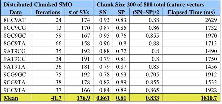
Multi-threaded chunking using different DNA hairpin datasets SVM Parameters: Gaussian kernel with sigma=.05, C = 10, Epsilon = .001, Tolerance = .001

This table shows the different multi-threaded chunking data runs performed on assortments of DNA hairpin pairs. The last line of the table presents the mean of the data runs to gauge the accuracy when using the Gaussian kernel.

8GC9AT 24 174 0.93 0.83 0.88 2629

8GC9CG 13 170 0.87 0.85 0.86 1732

8GC9GC 59 167 0.95 0.76 0.855 1970

8GC9TA 66 158 0.96 0.8 0.88 1713

9AT9CG 35 192 0.88 0.72 0.8 1490

9AT9GC 34 191 0.79 0.81 0.8 1750

9AT9TA 36 181 0.79 0.87 0.83 1456

9CG9GC 75 192 0.78 0.63 0.705 1912

9CG9TA 38 178 0.82 0.89 0.855 1533

9GC9TA 37 166 0.84 0.89 0.865 1922

(22)

Table 2.4

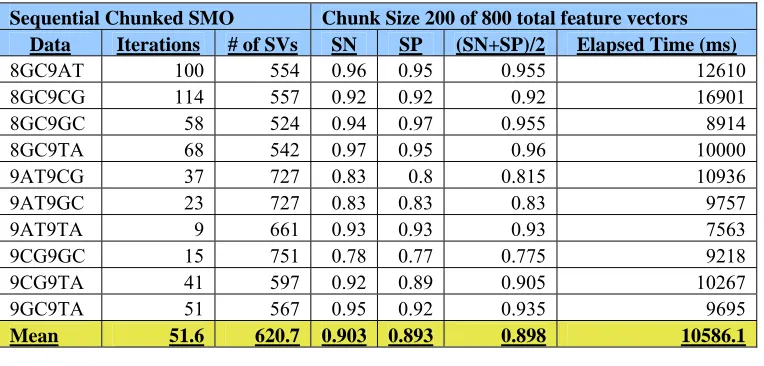
Sequential chunking using different DNA hairpin datasets SVM Parameters: Absdiff kernel with sigma=.5, C = 10, Epsilon = .001, Tolerance = .001

This table shows the different sequential chunking data runs performed on assortments of DNA hairpin pairs. The last line of the table presents the mean of the data runs to gauge the accuracy when using the Absdiff kernel.

Sequential Chunked SMO Chunk Size 200 of 800 total feature vectors Data Iterations # of SVs SN SP (SN+SP)/2 Elapsed Time (ms)

8GC9AT 100 554 0.96 0.95 0.955 12610

8GC9CG 114 557 0.92 0.92 0.92 16901

8GC9GC 58 524 0.94 0.97 0.955 8914

8GC9TA 68 542 0.97 0.95 0.96 10000

9AT9CG 37 727 0.83 0.8 0.815 10936

9AT9GC 23 727 0.83 0.83 0.83 9757

9AT9TA 9 661 0.93 0.93 0.93 7563

9CG9GC 15 751 0.78 0.77 0.775 9218

9CG9TA 41 597 0.92 0.89 0.905 10267

9GC9TA 51 567 0.95 0.92 0.935 9695

Mean 51.6 620.7 0.903 0.893 0.898 10586.1

Table 2.5

Sequential chunking using different DNA hairpin datasets SVM Parameters: Sentropic kernel with sigma=.5, C = 10, Epsilon = .001, Tolerance = .001

This table shows the different sequential chunking data runs performed on assortments of DNA hairpin pairs. The last line of the table presents the mean of the data runs to gauge the accuracy when using the Sentropic kernel.

8GC9AT 52 570 0.96 0.95 0.955 14479

8GC9CG 78 545 0.93 0.93 0.93 16844

8GC9GC 22 525 0.92 0.95 0.935 10065

8GC9TA 130 550 0.97 0.95 0.96 18304

9AT9CG 32 722 0.83 0.82 0.825 15273

9AT9GC 44 734 0.81 0.82 0.815 15452

9AT9TA 39 693 0.9 0.9 0.9 14419

9CG9GC 33 747 0.75 0.79 0.77 14855

9CG9TA 73 616 0.89 0.91 0.9 16978

9GC9TA 54 597 0.91 0.93 0.92 14159

(23)

Table 2.6

Sequential chunking using different DNA hairpin datasets SVM Parameters: Gaussian kernel with sigma=.05, C = 10, Epsilon = .001, Tolerance = .001

This table shows the different sequential chunking data runs performed on assortments of DNA hairpin pairs. The last line of the table presents the mean of the data runs to gauge the accuracy when using the Gaussian kernel.

8GC9AT 97 434 0.93 0.88 0.905 14978

8GC9CG 83 395 0.88 0.85 0.865 15653

8GC9GC 134 396 0.94 0.88 0.91 17783

8GC9TA 114 396 0.96 0.82 0.89 15988

9AT9CG 62 503 0.79 0.82 0.805 20789

9AT9GC 89 488 0.81 0.85 0.83 20833

9AT9TA 111 477 0.91 0.89 0.9 18057

9CG9GC 60 523 0.91 0.54 0.725 20233

9CG9TA 78 436 0.88 0.9 0.89 17910

9GC9TA 89 409 0.9 0.94 0.92 12422

Mean 91.7 445.7 0.891 0.84 0.864 17464.6

Table 2.7

Dataset = 9GC9CG_9AT9TA (1600 feature vectors) SVM Parameters: Absdiff kernel with sigma=.5, C = 10, Epsilon = .001, Tolerance = .001

Pass 100% of support vectors and 50% of polarization set Final Chunk Performance: {SN, SP} = {.87, .84}

This table shows the sequential chunking method focusing on the chunk sizes during the data run. The Absdiff kernel chunk performance is represented here. The breakdown of each feature vector set is displayed to show how the percentage parameters are used to pass portions of each set to the next chunk.

Chunk 1 Chunk 2 Chunk 3 Chunk 4

Total Chunk Size 400 787 1143 1472 Support Vectors 373 700 1002 1320 Polarization Set 27 86 140 152

Penalty Set 0 0 0 0

Violator Set 0 1 1 0

(24)

Table 2.8

Dataset = 9GC9CG_9AT9TA (1600 feature vectors) SVM Parameters: Sentropic kernel with sigma=.5, C = 10, Epsilon = .001, Tolerance = .001

This table shows the sequential chunking method focusing on the chunk sizes during the data run. The Sentropic kernel chunk performance is represented here. The breakdown of each feature vector set is displayed to show how the percentage parameters are used to pass portions of each set to the next chunk.

Support Vectors Passed 383 707 1011 Polarization Set Passed 9 43 70 Total Passed Set 392 750 1081

Table 2.9

Dataset = 9GC9CG_9AT9TA (1600 feature vectors)

SVM Parameters: Gaussian kernel with sigma=.05, C = 10, Epsilon = .001, Tolerance = .001

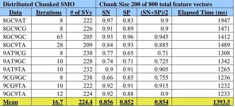
This table shows the sequential chunking method focusing on the chunk sizes during the data run. The Gaussian kernel chunk performance is represented here. The breakdown of each feature vector set is displayed to show how the percentage parameters are used to pass portions of each set to the next chunk.

(25)

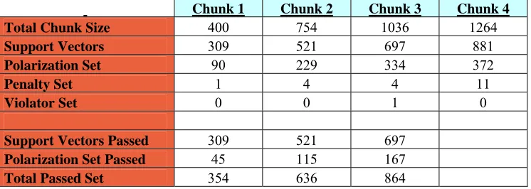
Table 2.10

Dataset = 9GC9CG_9AT9TA (1600 feature vectors) SVM Parameters: Absdiff kernel with sigma=.5, C = 10, Epsilon = .001, Tolerance = .001

This table shows the multi-threaded chunking method focusing on the chunk sizes during the data run. The Absdiff kernel chunk performance is represented here. The breakdown of each feature vector set is displayed to show how the percentage parameters are used to pass portions of each set to the next set of chunks.

C1 C2 C3 C4 C5 C6 C7 C8 C9 C10 Total Chunk Size 400 400 400 400 423 423 425 504 504 791 Support Vectors 373 377 378 388 402 402 403 466 460 699 Polarization Set 27 23 22 12 21 21 22 38 43 92 Penalty Set 0 0 0 0 0 0 0 0 0 0 Violator Set 0 0 0 0 0 0 0 0 1 0 Support Vectors Passed 1218 - - - 968 - - 742 - - Polarization Set Passed 53 - - - 40 - - 49 - - Total Passed Set 1271 - - - 1008 - - 791 - -

Table 2.11

Dataset = 9GC9CG_9AT9TA (1600 feature vectors) SVM Parameters: Sentropic kernel with sigma=.5, C = 10, Epsilon = .001, Tolerance = .001

This table shows the multi-threaded chunking method focusing on the chunk sizes during the data run. The Sentropic kernel chunk performance is represented here. The

breakdown of each feature vector set is displayed to show how the percentage parameters are used to pass portions of each set to the next set of chunks.

(26)

Table 2.12

SVM Parameters: Gaussian kernel with sigma=.05, C = 10, Epsilon = .001, Tolerance = .001

This table shows the multi-threaded chunking method focusing on the chunk sizes during the data run. The Gaussian kernel chunk performance is represented here. The breakdown of each feature vector set is displayed to show how the percentage

parameters are used to pass portions of each set to the next set of chunks.

C1 C2 C3 C4 C5 C6 C7 C8 C9 C10 Total Chunk Size 400 400 400 400 401 401 403 458 458 690 Support Vectors 291 309 316 305 318 320 313 341 354 495 Polarization Set 108 90 83 93 83 81 88 116 103 194 Penalty Set 1 1 1 0 0 0 2 1 0 1 Violator Set 0 0 0 2 0 0 0 0 1 0 Support Vectors Passed 980 - - - 764 - - 558 - - Polarization Set Passed 225 - - - 152 - - 132 - - Total Passed Set 1205 - - - 913 - - 690 - -

(27)

Chapter 3. Support Vector Reduction

3.1 Methods

Support Vector Reduction (SVR) is a process that is run right after the SVM learning step

is complete. Instead of going on to testing data against the training results to get accuracy, we

further reduce the support vector set. One way to do this is to coerce some alphas to zero which

means they would now fall into the polarization set and further away from the hyperplane.

Converting the smaller alphas to zeros makes the most sense since a larger alpha indicates that

the data point is stronger towards its grouping (polarized sign). This is done using a user-defined

alpha cut off value. All alpha values that are under the cut off are pushed to zero. It is not

entirely trivial since certain mathematical constraints must be met. The constraint that must be

met for this method is the linear equality constraint [2]:

0

1

=

∑

= N

i i i

y

α

Therefore, the alpha values not meeting the cutoff cannot just be forced to zero unless the

value is retained somewhere else in the set. This is done by first sorting the alpha values of the

support vectors. Then for each alpha that does not meet the cut off value, the small left over

value is added to the largest alpha of the same polarity. Since the list is sorted it can loop

through and evenly distribute the left over values through the larger alphas starting with the

largest. The reduction process can cut the support vector count down without significantly

affecting the accuracy. Other observations have shown that the easier the dataset to classify, the

(28)

3.2 SVR Results

Figure 3.1 shows the results of the SVR method on the non-chunking SMO SVM. For

this dataset, 0.19 seems like the best cut off value to use for future data runs since it retains the

accuracy while reducing the support vectors. As shown in Figure 3.1, the total run time

decreases as support vectors are reduced. This is due to a decrease in testing time since there are

not as many support vectors to test against. For the 9GC9CG_9AT9TA dataset, 140 support

vectors (10.5% of total) were dropped without affecting the accuracy.

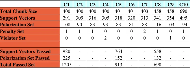
Data runs using sequential (Figure 3.3) and multi-threaded (Figure 3.2) chunking

methods with SVR show similar results. The chunking results tend to be a bit choppier since the

SVM algorithm makes some approximations thus the hyperplane will not be exactly the same for

every data run and this behavior is amplified in the chunking methods. Nonetheless, the trend

lines show that using the SVR method definitely cuts down on support vectors and decreases

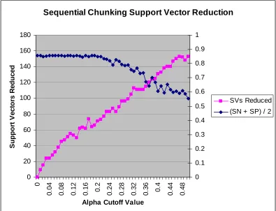
testing time. For sequential chunking (Figure 3.3), an alpha cut-off value of 0.25 caused 87

support vectors (7.2%) to be dropped without affecting accuracy. For multi-threaded chunking

(Figure 3.2), an alpha cut-off value of 0.22 dropped 26 support vectors (6.2%) while retaining

(29)

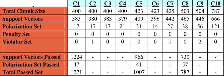
Figure 3.1

SMO (non-chunking) Support Vector Reduction Dataset: 9GC9CG_9AT9TA (1600 feature vectors) SVM Parameters: Absdiff kernel with sigma=.5, C = 10, Epsilon = .001, Tolerance = .001

This graph shows the rate of support vectors reduced as the alpha cutoff value is increased. The alpha cutoff value 0.19 is chosen as the best since it is the last value before accuracy begins to degrade. This chosen value reduces 140 support vectors.

SMO Support Vector Reduction

0 50 100 150 200 250 300 350 400 450 n/ a 0. 0 4 0. 0 8 0. 1 2 0. 1 6 0. 2 0. 2 4 0. 2 8 0. 3 2 0. 3 6 0. 4 0. 4 4 0. 4 8

Alpha Cutoff Value

(30)

Figure 3.2

Multi-threaded Chunking Support Vector Reduction

Dataset: 9GC9CG_9AT9TA (1600 feature vectors), Starting chunk size=400 SVM Parameters: Absdiff kernel with sigma=.5, C = 10,

Epsilon = .001, Tolerance = .001 Passing 30% of Support Vectors

Multi-threaded Chunking Support Vector Reduction

0 5 10 15 20 25 30 35 40 45 0 0. 0 4 0. 0 8 0. 1 2 0. 1 6 0. 2 0. 2 4 0. 2 8 0. 3 2 0. 3 6 0. 4 0. 4 4 0. 4 8

(31)

Figure 3.3

Sequential Chunking Support Vector Reduction

Dataset: 9GC9CG_9AT9TA (1600 feature vectors), Starting chunk size=400 SVM Parameters: Absdiff kernel with sigma=.5, C = 10,

Epsilon = .001, Tolerance = .001 Passing 100% of Support Vectors

Sequential Chunking Support Vector Reduction

0 20 40 60 80 100 120 140 160 180 0 0. 0 4 0. 0 8 0. 1 2 0. 1 6 0. 2 0. 2 4 0. 2 8 0. 3 2 0. 3 6 0. 4 0. 4 4 0. 4 8

(32)

Chapter 4. SVM Chunking

SVM chunking provides an alternative method to running a typical SVM (SMO) on a

dataset by instead breaking up the training data and running the SVM on smaller chunks of data.

In the chunking process, feature vectors associated with strong data points are retained from

chunk to chunk, while weak data points are discarded. Chunking becomes a necessity when

classifying large datasets. In this context, a large dataset refers to one that has over 5,000

features vectors where each vector has 150 components. Since the order of computations

increases by the square of the size of the training set, most PCs would not have enough memory

to support a kernel matrix of 10,000 or more training instances.

Initially, the training data is shuffled then broken into chunks. The number and size of the

chunks depends on the size of the dataset to be trained. In the Java implementation of this

algorithm, the user specifies the size of each chunk and the chunks are broken up accordingly. If

the chunks don't divide evenly, which is the case most of the time, the few remaining feature

vectors are added to the last chunk. When training on the chunk is complete, the resulting

trained feature vectors each fit into a separate set. If the SVM classifies well, the largest set

consists of the support feature vectors. The KKT violators make up another set. KKT violators

refer to feature vectors that violate one of the KKT relations. The violator set is usually zero at

the end of the training process, unless some minimal number of violators is allowed upon

learning completion. The polarization set consists of the feature vectors that have been classified

as a positive or negative one. These are feature vectors that pass the KKT relations and have an

alpha coefficient equal to zero. The penalty set consists of the feature vectors which pass the

KKT relations and have alpha coefficients equal to C (the max value). These sets give the user a

(33)

converging to a better solution, on the next chunk run, several support feature vectors and

sometimes some of the polarization set are passed to the next chunk(s). The percentages of each

feature vector set depend on which kernel is used and the dataset.

There are different methods of extracting the feature vectors from the different sets. The

specified percentages of feature vectors are pseudo-randomly chosen from each of the sets

except for one. The support feature vectors extraction method differs since it extracts the feature

vectors that have the best scores. Each score represents the distance of the feature vector from

the hyperplane. It makes sense to choose feature vectors whose scores are closer to the

hyperplane in order to pass a tighter hyperplane on to the next chunk(s). Passing a more precise

hyperplane should speed up the next SVM run.

4.1 Previous SVM chunking methods

Zanghirati and Zanni [6] developed the variable projection method (VPM) for training

SVMs in parallel. This method is based off of Joachim's SVM light decomposition techniques

[7] which delve further into the inner workings of the SMO algorithm [2]. First, the feature

vector indices are divided into two categories, the free and fixed sets based upon their alphas

(Langrange Multipliers). The free set represents the KKT violators which need to be further

optimized while the fixed set is the alphas that already fulfill the KKT equations. An alpha

variable from each set is used to solve each quadratic sub problem in order to optimize the free

set alphas until convergence. Though this sounds similar to Platt's SMO [2], Joachim performs

some additional tricks to cut down on the number of iterations needed to converge [7]. VPM

provides a parallel solution to computing the kernel matrix which is the most memory intensive

part of the SVM. The kernel calculations are spread among several processing elements and the

(34)

elements. Since the rows are duplicated, they must be synchronized after each local

computation. VPM is implemented using standard C and MPI communication routines.

Hans Peter Graf et al. [9] developed the Cascade SVM to parallelize SVMs. This method

begins by breaking the large dataset into chunks. The SVM is run on each separate chunk in the

first layer. When the SVMs have all converged, new chunks are created from the resulting

support vectors from the pairs of first layer chunks which make up the second layer of chunks.

This occurs until a final chunk is reached. The final set of support vectors is then fed back into

each first layer chunk. If further optimization is possible and needed, the entire process is rerun

until the global optimum is met. If the global optimum is not needed due to decent initial

training results, the process can be halted after one run of the network of chunks. Allowing the

Cascading SVM to continue running will eventually produce the global optimum. This method

seems intuitive but after testing, we have found that passing 100% of support vectors down to the

next set of chunks without also passing some non support vectors or using the SVR method does

not work properly with the DNA hairpin data used here. The data run never finishes, in fact,

since it cannot further reduce the support vectors to converge to the final chunk. This weakness

of the method, not apparent at first sight or mentioned in [9], may be understood if the SVs from

different chunks are sufficiently different and training on SVs from individual chunks are

(35)

As shown in the illustration, the actual margins for each chunk (between the two green

lines) are not recognized since another significant margin exists. The SVM continually works on

trying to fit the hyperplane between the intercalating chunk margin (between the red dashed

lines) and never finishes running.

Illustration 4.1

100% SV Passing for multi-threaded chunking without SVR

+ + ₊ ₊ + +

+

- - - -

+

- -

The chunking methods presented here have some similarities to the Cascade SVM. As

discussed above, the large dataset is broken into smaller chunks and the SVM is run on each

separate chunk. Instead of bringing the results of paired chunks together, all chunk results are

(36)

chunk is calculated which gives the trained result. Since SVM parameters vary for different

datasets, the user has the option to tune the percentage of support vectors and non support

vectors to pass to the next set of chunks. Additionally, passed support vectors are chosen wisely

to produce a tighter hyperplane to better distinguish the polarization sets. Another aspect not

covered in the Cascade method is the SVR method. This method runs as part of the core SVM

learning task on each chunk. It uses a user-defined alpha cutoff value for further tuning and can

significantly reduce the number of support vectors passed to the next set of chunks. These

additional steps reduce the size of the chunks thus making the algorithm run faster without loss

of accuracy. Details of these steps are discussed in more depth in chapter 3.

4.2 Sequential Chunking (Linear Topology)

Sequential chunking is one form of chunking which is not multi-threaded. This method

runs the SVM on the first chunk, and then sends the support feature vectors (SVs) and sometimes

non-SVs to be added onto the training data for the next chunk. This continues until the final

chunk has been run. When using sequential chunking, feature vector passing can be difficult

since passing too many features on to the next chunk can result in large datasets in the later

chunks in the process. Support feature vectors are the most valuable to pass to the next chunk

since they define the hyperplane.

4.3 Sequential Chunking Results

For the DNA hairpin datasets used here, results have shown that the ideal chunking

parameter for sequential chunking is 100% of the support vector set. This produced the best

accuracy (0.855) within stable conditions (Figure 4.1). Illustration 4.2 displays a sample run and

the size of each chunk as the algorithm progresses through the chunks. Table 2.7 shows the

(37)

Illustration 4.2 Linear Topology Chunk Progression

Training Training Training Final

Chunk 1 Chunk 2 Chunk 3 Chunk

400 features 787 features 1143 features 1472 features

Figure 4.1

SVM Parameters: Absdiff kernel with sigma=.5, C = 10, Epsilon = .001, Tolerance = .001 This shows the trend for sequential chunking when using different support vector and

polarization set percentage parameters. Every variation of multiples of ten up to 100 was used for each of the two sets. For example, when the SV % parameter was 10, the polarization set % parameter would vary from 0 to 100 in multiples of ten. For most of the data run, especially the more stable part at 100 % SVs, the variation of the polarization set did not seem to have much effect on the outcome.

Sequential Chunking % Parameters

0.74 0.76 0.78 0.8 0.82 0.84 0.86 0.88

10 10 10 20 20 30 30 40 40 50 50 60 60 60 70 70 80 80 90 90 ₁₀0 ₁₀0

Support Vector % Passed

(S

N

+

S

P

)/

2

(38)

4.4 Multi-threaded Chunking (Binary Tree Topology)

The multi-threaded chunking method simultaneously runs the chunks using multiple

threads. Once all of the threaded chunks are finished training, the chunk results are collected

into an array. The same user defined percentages of feature vector sets are used here except this

time those percentages of feature vectors are extracted from each chunk. All of the chosen

feature vectors to be passed are stored together then re-chunked if the current data set is large

enough to be chunked again. Re-chunking occurs when the data set is greater than or equal to

twice the specified chunk size. If this is not the case, the final chunk is run alone to get the final

result. The main use of the multi-threaded chunking method is with a single computer with

multiple processors/cores.

Observations have shown that sending 100% of the support vectors to the next chunk

generally causes the chunking to run continuously without ever ending with a result. At least, on

these challenging datasets, this is an expected behavior since passing all support vector data to

the next chunk level would just be re-chunking the same support vectors that were already done

the first time. Some data must be dropped to converge to the final chunk whether it is through

the chunking parameters or the SVR method. Dropping too much data can affect the final

accuracy while retaining too much data increases training time. Therefore the chunking

(39)

4.5 Multi-threaded Chunking Results

The best accuracy result (0.83) within stable conditions for multi-threaded chunking were

obtained using 30% of the support vectors set as shown in Figure 4.3. Illustration 4.3 displays a

sample multi-threaded chunking run and the size of each chunk as the algorithm progresses

through the sets of chunks.

Illustration 4.3 Binary Tree Topology Chunk Progression

The numbers in each chunk represent the number of feature vectors (fv).

Training Training Training Training

400 fv 400 fv 400 fv 400 fv

Training Chunk 5

520 fv

Training Chunk 6

512 fv

Final Chunk 7

743 fv Specified fv passed to

the next chunks

Specified fv passed to the last chunk

(40)

Figure 4.2

SVM Parameters: Absdiff kernel with sigma=.5, C = 10, Epsilon = .001, Tolerance = .001 This shows the trend for multi-threaded chunking when using different support vector and polarization set percentage parameters. Every variation of multiples of ten up to 100 was used for each of the two sets. For example, when the SV % parameter was 10, the polarization set % parameter would vary from 0 to 100 in multiples of ten. For most of the data run, especially the more stable part at 30 % SVs, the variation of the polarization set did not have much effect on the outcome.

Multi-threaded Chunking % Parameters

0.72 0.74 0.76 0.78 0.8 0.82 0.84 0.86

10 10 10 20 20 30 30 40 40 50 50 60 60 60 70 70 80 80 90 90 ₁₀₀ ₁₀0

Support Vector % Passed

(S

N

+

S

P

)/

2

(SN+SP)/2

4.6 Multi-threaded Distributed Chunking

Multi-threaded distributed chunking is a multi-server/multi-CPU (core) approach to the

previous multi-threaded chunking method. Java RMI is used to handle the remote calls between

the client and servers. The client program runs multi-threaded remote calls to a user specified set

(41)

When the client program runs, a chunk is passed to each available processor/core in the network

until all or as many as possible are training simultaneously. As the chunks finish, the results are

passed back to the client. Each “chunk level” may take multiple batches depending on the chunk

size and amount of processors/cores available. The final chunk is largest so the client program

should be processed on the machine with the most computing power. This not only speeds up

the final chunk but allowing larger chunks should produce better final results. The main benefit

of this method is a significant decrease in run time for large datasets. As shown below in Table

4.1, multi-threaded distributed chunking performs well when it comes to run time. Network

overhead causes it to be slightly slower than the non-remote multi-threaded chunking method.

With extremely large datasets (i.e. 60,000 feature vectors), the Remote method would be faster.

Table 4.1

SVM Parameters: Absdiff kernel with sigma=.5, C = 10, Epsilon = .001, Tolerance = .001 For chunking methods: Pass 90% of support vectors,

Starting chunk size = 400, maxChunks = 2

For SV Reduction methods: Alpha cut off value = .15

This table shows the overall performance of the different SVM methods. The distributed chunking had three identical networked machines (see Appendix for details).

SVM Method Sensitivity Specificity (SN + SP) / 2

Total Time (ms)

SMO (non-chunked) 0.87 0.84 0.86 47708

Sequential Chunking 0.84 0.86 0.85 27515

Multi-threaded Chunking 0.88 0.78 0.83 7855

SMO (non-chunked) with SV

Reduction 0.91 0.81 0.86 43662

Sequential Chunking with SV

Reduction 0.90 0.82 0.86 18479

Multi-threaded Chunking with SV

Reduction 0.85 0.83 0.84 5232

Multi-threaded Distributed Chunking

(42)

Chapter 5. Conclusion

Support Vector Machines are extremely useful for classifying data and therefore

dominating over other methods in a variety of fields and applications. Since the main weakness

of SVMs is the long training time when running large datasets, it is only natural that one would

develop multi-threaded distributed methods especially since many typical computers today have

multiple cores/processors, each with a continuously growing capacity for RAM.

An overall comparison of the SVM methods explained here can be found in Table 4.1

(above). Sequential chunking has the benefit of holding onto accuracy when compared to

running the straight SVM (SMO) but the run times can be higher since the method does not run

in parallel. Though this performance hit is significantly countered when using the SVR method.

Another benefit of sequential chunking is that it helps cut down on high memory usage for the

kernel matrix build which can make the difference since the straight SVM may bog down from

hard drive thrashing if the machine does not have enough memory. The only negative aspect is

that chunk size can still eventually grow too much for extremely large datasets so the chunking

percentage parameters must be adjusted accordingly.

Multi-threaded chunking has a significant run time performance increase which is further

improved when employing the SVR method. The multi-threaded aspect allows training of

extremely large datasets which may not be possible using sequential chunking. Additionally,

using the multi-threaded distributed method allows users to add several more machines to make

the algorithm train even faster. This aspect makes the size of the dataset no longer a concern for

SVM training, which opens up the practical use of SVM methods to more applications than

(43)

References

[1] Winters-Hilt, S., Yelunder, A., McChesney, C., and Landry, M., “Support Vector Machine Implementations for Classification & Clustering”, BMC Bioinformatics, (2006).

[2] Platt, J.C., “Sequential Minimal Optimization: A Fast Algorithm for Training Support Vector Machines”, Microsoft Research, Technical Report MSR-TR-98-14, (1998).

[3] Osuna, E., Freund, R., and Girosi, F., “An Improved Training Algorithm for Support Vector Machines”, Proc. IEEE NNSP ’97, (1997).

[4] Vapnik, V., Estimation of Dependencies Based on Empirical Data, Springer-Verlag, (1982).

[5] Cortes, C., Vapnik, V., “Support Vector Networks”, Machine Learning, 20:273-297, (1995).

[6] Zanghirati, G., Zanni L., “A parallel solver for large quadratic programs in training support vector machines”, Parallel Computing, Vol. 29, pp.535-551, 2003.

[7] Joachims, T., Making large-scale SVM learning practical, in: B. Sch€lkopf, C.J.C. Burges, A. Smola (Eds.), Advances in Kernel Methods––Support Vector Learning, MIT Press, Cambridge, MA, 1998.

[8] Platt, J.C., Fast training of support vector machines using sequential minimal optimization, in: B. Sch€lkopf, C. Burges, A. Smola (Eds.), Advances in Kernel Methods––Support Vector Learning, MIT Press, Cambridge, MA, 1998.

[9] Graf, H.P., Cosatto, E., Bottou, L., Durdanovic, I., Vapnik, V., Parallel Support Vector Machines: The Cascade SVM, in proceedings NIPS, 2004

[10] Vapnik, V., The Nature of Statistical Learning Theory, Springer-Verlag, New York, 1995.

[11] Joachims, T., "Text Categorization with Support Vector Machines", LS VIII Technical Report, No. 23, University of Dortmund, (1997).

[12] Osuna, E., Freund, R., Girosi, F., "Training Support Vector Machines: An Application to Face Detection," Proc. Computer Vision and Pattern Recognition ’97, 130-136, (1997).

[13] LeCun, Y., Jackel, L. D., Bottou, L., Cortes, C., Denker, J. S., Drucker, H., Guyon, I., Muller, U. A., Sackinger, E., Simard, P. and Vapnik, V., "Learning Algorithms for

Classification: A Comparison on Handwritten Digit Recognition," Neural Networks: The Statistical Mechanics Perspective, Oh, J. H., Kwon, C. and Cho, S. (Ed.), World Scientific,

(44)

Appendix

Note 1: All data sets used in this paper were recorded in the Winters-Hilt Children’s Hospital

laboratory using a nanophore detector. This raw data was then fed through a Hidden Markov

Model which produced the feature vectors.

Note 2: All data runs (except for Table 4.1) were done on a (PC) machine with Debian Linux

containing dual AMD Athlon MP 2400 (2 ghz.) processors with 2 gigabytes of RAM.

Note 3: The Table 4.1 data runs were done using three Sun machines with Ubuntu Linux each

containing a quad processor, dual core AMD Opteron 280 (1 ghz.) processor with 8 gigabytes of

RAM.

A.1 Java code implementation of sequential chunking method

SequentialChunksSVM.java

package edu.uno.cs.bioinformatics.svm.chunking;

import cern.colt.list.IntArrayList;

import edu.uno.cs.bioinformatics.data.ModelParameters; import edu.uno.cs.bioinformatics.data.TrainingData; import edu.uno.cs.bioinformatics.svm.SVMModel; /**

* The SequentialChunkTrial breaks up the training data and runs the SVM on the chunks.

* The chunks are trained in sequence in order to pass support features to the next chunk.

*/

public class SequentialChunksSVM extends AbstractChunksSVM {

static final long serialVersionUID = 25123L;

private ChunkParameters chunkPar; private TrainingData trainingData; private ModelParameters param; private SVMModel model;

private ChunkResult chunkRes; private SVMchunkLearner svmEngine; private SVMchunkLearner newEngine;

/**

* The feature vector indices that are */

private IntArrayList penaltySet = new IntArrayList();

(45)

*/

private IntArrayList polarizationSet = new IntArrayList();

/**

* The feature vector indices that are KKT violators. */

private IntArrayList kktViolators = new IntArrayList();

/**

* The support feature vector indices. */

private IntArrayList svList = new IntArrayList();

/**

* Save the first chunk to use for testing in order to verify the integrity of the chunking process.

*/

protected TrainingData firstChunk;

/**

* Constructs a new sequential chunk trial with the given SVMLearner, TrainingData, and Parameters.

* @param maxSize the maximum size of each chunk

* @param trainingData the feature vectors and labels to train on * @param param the user defined parameters object

*/

public SequentialChunksSVM(SVMchunkLearner svmEngine, ChunkParameters chunkPar, TrainingData trainingData, ModelParameters param) {

this.svmEngine = svmEngine; this.chunkPar = chunkPar;

this.trainingData = trainingData; this.param = param;

} /**

* Default Constructor */

public SequentialChunksSVM() {}

/**

* The runSeqChunkedSVM method runs the SVM chunks sequentially. * @return the results model

*/

public SVMModel runSeqChunkedSVM() {

int featsCount = trainingData.getLabels().size();

int chunkCount = (int)Math.ceil((featsCount*1.)/(chunkPar.chunkSize*1.)); TrainingData[] data = makeDataChunks(chunkCount);

this.firstChunk = data[0];

String resCapture = "Chunk Number\tChunk Size"; int chunkTally = 0;

//traverse through the chunks for (int i=0; i<chunkCount; i++) {

Distributed Support Vector Machine Learning

ScholarWorks@UNO

ScholarWorks@UNO

Distributed Support Vector Machine Learning

Distributed Support Vector Machine Learning

Acknowledgment

Table of Contents

List of Figures

List of Tables

List of Illustrations

Abstract

Keywords

Chapter 1. Introduction

Chapter 2. Support Vector Machines

2.1 Introduction

2.2 Applications of Support Vector Machines

2.3 Derivation of Binary SVM [1]

b)

w

w

(

2

w

w

b;

(w,

α

)

=

−

α

y

−

−

α

L

=

∑

α

α

α

γ

α

ξ

α

ξ

µ

ξ

µ

ξ

α

)

=

−

y

−

+

+

+

C

−

L

[

(

w

x

b)

]

2

w

w

,

,

b;

(w,

=

∑

ξ

ξ

=

_α

_ξ

_α

_ξ

_µ

_ξ