Applying inversion techniques to derive source currents and geoelectric fields for geomagnetically induced current calculations

www.ann-geophys.net/32/1263/2014/ doi:10.5194/angeo-32-1263-2014

© Author(s) 2014. CC Attribution 3.0 License.

Applying inversion techniques to derive source currents and

geoelectric fields for geomagnetically induced current calculations

J. S. de Villiers and P. J. Cilliers

SANSA Space Science, P.O. Box 32, Hermanus 7200, South Africa Correspondence to: J. S. de Villiers ([email protected])

Received: 23 January 2014 – Revised: 17 August 2014 – Accepted: 3 September 2014 – Published: 16 October 2014

Abstract. This research focuses on the inversion of geomag-netic variation field measurement to obtain source currents in the ionosphere. During a geomagnetic disturbance, the iono-spheric currents create magnetic field variations that induce geoelectric fields, which drive geomagnetically induced cur-rents (GIC) in power systems. These GIC may disturb the operation of power systems and cause damage to grounded power transformers. The geoelectric fields at any location of interest can be determined from the source currents in the ionosphere through a solution of the forward problem. Line currents running east–west along given surface position are postulated to exist at a certain height above the Earth’s sur-face. This physical arrangement results in the fields on the ground having the magnetic north and down components, and the electric east component. Ionospheric currents are modelled by inverting Fourier integrals (over the wavenum-ber) of elementary geomagnetic fields using the Levenberg– Marquardt technique. The output parameters of the inversion model are the current strength, height and surface position of the ionospheric current system. A ground conductivity structure with five layers from Quebec, Canada, based on the Layered-Earth model is used to obtain the complex skin depth at a given angular frequency. This paper presents pre-liminary and inversion results based on these structures and simulated geomagnetic fields. The results show some inter-esting features in the frequency domain. Model parameters obtained through inversion are within 2 % of simulated val-ues. This technique has applications for modelling the cur-rents of electrojets at the equator and auroral regions, as well as currents in the magnetosphere.

Keywords. Geomagnetism and paleomagnetism (geomag-netic induction) – ionosphere (electric fields and currents; modeling and forecasting)

1 Introduction

Solar events, such as coronal mass ejections that become geo-effective, create disturbances within the Earth’s magne-tosphere giving rise to geomagnetic storms and substorms. During geomagnetic storms, the compression of the magne-tosphere by the solar wind and the interaction of the solar wind with the Earth’s magnetic field enhance the currents in both the magnetosphere and ionosphere. These currents cause fluctuations in the electric and magnetic fields on the ground. The equatorial electrojet is at 100 km in the iono-sphere. The ionosphere extends up to∼1000 km and has cur-rent systems that lie at a height of∼100 km. Rapid changes in the geomagnetic field generate geoelectric fields that drive geomagnetically induced currents (GIC) in power lines. The GIC have the potential of causing transformers to fail, with subsequent consequences of a power blackout to the general public, who are increasingly reliant on electrical power for their everyday operations and living (Albertson et al., 1993; Shea and Smart, 1996; Wilkinson, 2007; Withbroe, 2001).

Therefore, it is of interest to power utility operators that a warning system be developed that can predict GIC, which may occur after an eruptive event occurs on the sun. Because of the complexities involved in such a solar–terrestrial inter-action and the tremendous challenges facing such a project, we consider as a first step the inversion of the geomag-netic field observations to obtain ionospheric source currents. From these source currents, we estimate the induced geoelec-tric fields as measured at any location of interest, particularly the electric fields responsible for GIC in power grids on the ground.

geomagnetic data are readily available for many locations on Earth (Kerridge, 2001; INTERMAGNET, 2014) where there are magnetometers, but conductivity structures for the calcu-lation of surface impedances are scarcer. Therefore, geoelec-tric data obtained by the direct method are valid locally only (see Fig. 1).

The inversion method allows us to compute geomagnetic fields, via Fourier integrals, at any location of interest. For this to work, a 1-D planar conductivity structure obtained for one location is assumed to be valid everywhere over the rel-evant region (see Fig. 1 again). From the conductivity struc-ture, a surface impedance or skin depth is computed.

The motivation for using the field inversion method de-scribed in this paper is that the geomagnetic measurement for calculating the geoelectric field that drives GIC in power systems is generally not available at the location of interest. Once the parameters of the current system are determined by the inversion from geomagnetic data, one can return to the forward problem Fourier integral and use these parameter values to calculate the geomagnetic field anywhere (the curve in Fig. 1). Inversion provides an alternative way in which to estimate the geomagnetic fields where it is not possible by other means.

Either the electric field can be obtained through a direct multiplication of the spectrum of the magnetic field with the relevant components of the surface impedance at the loca-tion of interest, or via the Fourier integral, using a reflecloca-tion coefficient derived from a model of the ground conductivity. It can be shown that the electric fields are the same when the exact expression for the reflection coefficient is used in the Fourier integrals. But, when the reflection coefficient is replaced with an exponential approximation to facilitate the analytic solution of the integrals, the electric fields obtained are actually different. These differences are addressed in this paper.

A general theoretical framework for computing the fields due to an ionospheric electrojet above a layered Earth was proposed by Hakkinen and Pirjola (1986). To simplify com-putations, we use the complex image method (CIM), intro-duced by Wait and Spies (1969) and used by Thomson and Weaver (1975) to replace a conducting planar model for lay-ered Earth by an image current placed at a depth equal to the height of the current system above the Earth plus twice the complex-valued skin depth associated with electromagnetic waves penetrating the Earth. Pirjola and Viljanen (1998) took this approach and applied it to a finite auroral electrojet with field-aligned currents carrying away excess charges to or from the magnetosphere in the Northern Hemisphere.

This paper takes the simulated magnetic data from Boteler et al. (2000) and use inversion techniques in the complex im-age method to obtain the current strength (and position) of the modelled auroral electrojet. For this purpose we take this ionospheric current to be a line current above the Earth. The planar model in the Cartesian coordinate system with a line current above a layered Earth is a local approximation of a

ܤ௫ ܧ௬

ℎଵ ߝଵ

ߪଵ ߤଵ

ℎଶ ߝଶ

ߪଶ ߤଶ

x x

Inversion fit Inversion estimate

ܧ௬ݔ௜, ߱ = −ܼ(߱)ܤ௫ݔ௜, ߱ /ߤ

ܼ(߱) = constant

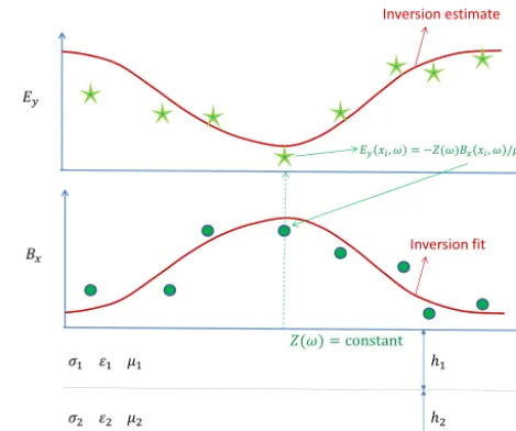
Figure 1. A conceptual diagram to illustrate the following: (1) the surface impedance for a layered medium independent of positionx, (2) the electric fieldEycan be determined from the direct relation

Ey(xi, ω)= −Z(ω)Hx(xi, ω)(shown as stars) based on the mea-sured magnetic field (shown as dots), (3) the electric field and the magnetic field (shown as solid lines) can be determined from the Fourier integrals of the currents obtained from the inversion of the measured magnetic field, (4) the direct and indirect methods give approximately the same values for the electric field.

ring current around the Earth. No field-aligned currents are considered here.

2 Theory

We introduce an inversion approach on simulated magnetic data to obtain ionospheric current system characteristics. The application of the CIM allows one to approximate the re-flection coefficient to an exponential. It is dependent on the skin depth, and thus the surface impedance. The surface impedance can be computed for one fixed frequency by using the Quebec conductivity structure in Canada (see Hakkinen and Pirjola, 1986), which is based on the general theory for computing the geomagnetic and geoelectric fields due to an electrojet in the magnetosphere above a layered Earth. Ap-pendix A contains details of the relevant derivations of the theory.

We restate the expressions of Eq. (A9) here:

Bx, Bz T

(x, ω)=

I µ 2π

h+2p, xT (h+2p)2+(x−xo)2

+ [h,−x] T

h2_+(x−x

o)2

!

, (1)

wherexis the latitude andωis the frequency. The parameters areIthe ionospheric current strength,hthe height,xothe

The functionp (ω)is the complex skin depth that depends on the conductivity structure. The transpose of a vector is indi-cated by the symbolT.

The Fourier integral expression of ground magnetic field components (Eq. 1) is the model function in the inversion problem that obtains the output parameters (I,h,xo)of the

model for a line current system above the Earth. These pa-rameters, once found, are substituted into the ground geo-electric field expression for estimation:

Ey(x, ω)= iω

2 I µ 2πln

h2+(x−xo)2 (h+2p)2+(x−xo)2

!

. (2)

3 Methodology

3.1 Forward procedure

A model comprises entities and relations defined by variables and parameters. Entities include the currents, the fields and the Earth. The relations between these entities in the for-ward problem are Eqs. (1) and (2). The input variables to these equations are the surface distancex and frequencyω. Output variables are the electric and magnetic fields. The skin depth p is dependent on frequency ωand two sets of parameters: conductivities σn plus half-space conductivity σN+1, and thicknesseshnfor leveln=1, . . ., N of a layered

structure of the Earth. The other parameters are the current strengthI and heighth. The equations have been altered to include another parameter: the positionxoof the current

sys-tem. Then,x is replaced byx−xo, here. Therefore, the

pa-rameterxoshifts the fields along the surface in either

direc-tion.

Before any inversion can be performed, reference mag-netic data must be obtained against which the inversion can be tested. The test data were obtained by calculating Eq. (1) to replicate the physical set-up of Boteler et al. (2000). In this reference, the physical set-up was a Cauchy distributed cur-rent system 100 km above the Earth with a spread of 200 km. Thus, the line current system for this study should be 300 km high to produce the same results. These data have a sur-face range from −1000 to+1000 km with a grid spacing of 50 km. They can be regarded as a string of magnetome-ter stations at positionsxi along a meridian. Take note that

the modelled curves are symmetric aroundxo=0 km forBx

andEy, and antisymmetric forBz. The current strength was

assumed to be 103kA.

For a Quebec conductivity structure and fluctuation pe-riod of τ=5 min, skin depthp(τ;[hn, σn])and impedance Z(τ;[hn, σn])estimates were obtained and passed along to

the field Eq. (1). Here the skin depth and impedance de-pend on the following variables:τ is the fluctuation period and [hn, σn] is the set of conductivitiesσn plus half-space

conductivityσN+1, and thicknesseshnfrom the conductivity

structure.

The results of the forward computations are given in Sect. 4.

3.2 Inversion fundamentals

Usually we have a data set d and a model design set m

related to each other by an operation F through the rela-tiond=F(m). This defines the forward problem. We only have available the observationsd. The process has to be in-verted for m=F−1(d)=G(d), and that requires optimi-sation techniques and an objective function G(d). This de-fines the inverse problem. For a more comprehensive descrip-tion of the theory, consult Chave and Jones (2012). See also Taranatola (2005).

The linear inverse problems take the form d=Fm or

m=Gdin which case F and G are matrices andmanddare column vectors. These matrices are constant with respect to

mandd. However, the optimisation is in general of a nonlin-ear nature. Some approaches take advantage of linnonlin-ear meth-ods by considering a linearised form of the inverse problem. This is accomplished by expanding F(m)in a Taylor series around a reference modelm∗:

F(m)=F(m∗)+Jm∗(m−m∗)+o(km−m∗k), (3) where Jm∗ is a Jacobian matrix with

Jm∗

ij= ∂Fi(m) /∂mj

m=m∗. The

k·k is the norm of a vector andois the Landau operator from asymptotic theory on the norm of the model differencem−m∗. A linearised inverse problemF is formed when only the first two terms in Eq. (3)¯ are retained and the higher-order terms are discarded. F is¯ then an affine transformation: a linear transformation plus a constant.

3.2.1 Errors and standard deviations

Adding an error vectorto the data givesd˜=F(m)+. This alters the inversion relation to include errors in the model:

˜

m=Gd˜. The notion of well-posed problems (forward and inverse) was established by Hadamard (1902). The con-ditions for well-posed are a solution to a problem must (1) exist, (2) be unique, and (3) be stable. Failure of any one of these conditions results in an ill-posed problem. Thus, we have a forward problemd˜=F m˜

. The F maps a subset of vectors in model space (the domain of F)to a subset of vec-tors in the data space (the range of F). The existence ofm˜ means thatd˜ must be in the range of F. The uniqueness of

˜

mfollows when F has a one-to-one transformation, mapping different vectors in model space to different vectors in data space. Then the solution is given by m˜ =F−1d˜, where F−1is defined such that its domain is in the range of F. The stability ofm˜ pertains to the effect of the erroronm˜. When error-free (=0), thenm˜ =F−1(F(m))=m; that is, the so-lution is not only unique, it is correct. In general, however,

Stability requires that the solution error be bounded when the data error is bounded as well. Thus,m˜ is stable when a positive functionε(µ)exists, such thatkδmk_{< µ}whenever kk< ε(µ). This is a definition for the continuity transfor-mation:m˜ is stable when F−1is continuous.

It is possible to calculate variances and standard devia-tions of the output parameters in the model. The variances and deviations are obtained from a covariance matrix for parameters. We start with the error vector of residuals = [r1, r2, . . ., rN]. The residualsri are computed by taking the

difference between the data and the forward problem func-tion, where N is the number of data. A Jacobian matrix J is formed by partial differentiating of the objective func-tion with respect to each of its parameters for a set of data pointsxi. Then the deviation of the fittedmfrom the actual

˜

m parameter vector position for the minimum of the objec-tive function is

µ=m−m˜ =J−1+o(kk). (5)

Neglecting higher power terms ofkk, we multiplyµwith its transpose:

µµT =hJ−1i hJ−1iT =hJ−1iThJ−1iT. (6)

The sum-of-squared residuals (SSR) are obtained from the corresponding multiplication ofwith its transpose:T ₌

PN

i ri2=N sSSR. Here the SSR variation issSSR.

Substitut-ing this into Eq. (6) and dividSubstitut-ing byN, the parameter covari-ance matrix6is formed:

6=hJ−1i XN

i r

2

i/N

h

J−1iT =sSSR

h

JTJi −1

. (7)

The variance for the parameters can then be obtained from the diagonal elements of6. The square roots of the diagonal elements are the parameter standard deviations.

3.2.2 An optimisation problem

An optimisation in a simple case is a minimisation or max-imisation of a function describing some system character-istic (say a physical property) dependent on m. In an ad-vanced case the objective function f(d, m) might then be subject to equality fη(d, m)=0[η=1, . . ., N]and

inequal-ity fµ(d, m)≤0[µ=1, . . ., M]constraints and/or parameter

boundsmLandmH. A general problem description may be

stated as follows:

f(d, m),subject tomL≤m≤mH, (8)

fη(d, m)=0[η=1, . . ., N],

fµ(d, m)≤0 [µ=1, . . ., M].

This is a minimisation problem. Most optimisation tech-niques are designed to be minimisation techtech-niques. Maximis-ing the objective function instead requires that function to be

negated and the negative function be then minimised again, e.g. f(d, m)=[−f(d, m)]. The inequality constraints may be negated as well, that is fµ(d, m)≥0 [µ=1, . . ., M].

An efficient and accurate solution to this problem depends not only on the size of the problem in terms of the num-ber of constraints and model design parameters, but also on the characteristics of the objective function and constraints. When both f(d, m) and fη,µ(d, m)are linear functions of

the model vector, the problem is known as a Linear Optimi-sation (LO) problem. Quadratic OptimiOptimi-sation (QO) concerns the optimisation of a quadratic objective function with lin-ear constraints. For both types of problems, reliable solution procedures are readily available, such as the decomposition methods. More difficult to solve are Nonlinear Optimisation (NO) problems, in which f(d, m)and fη,µ(d, m)can be

non-linear functions of the model vector. A solution of the NO problem generally requires an iterative technique to establish a search direction. This is usually achieved by an approxi-mate solution of an LO, a QO or unconstrained sub-problem. 3.2.3 Least-squares problems

When the optimisation problem is a least-squares prob-lem, the objective function f(d, m)assumes the form of a sum-of-squares function of residuals. That is for datad= (d1, d2, . . ., dN)and modelm=(m1, m2, . . ., mM):

f(d, m)=XN i=1r

2

i =

XN

i=1(Fi(m)−di)

2_{. (9)} The same constraints apply and fη,µ(m)are arbitrary

func-tions.

Linear least squares will not be used in this study, so de-composition techniques does not apply. One has to rely on iterative optimisation algorithms. Many iterative techniques can be applied on nonlinear least-squares inversion prob-lems. These require much computational work, representing the different methods in which a nonlinear model starts at an initial guess positionms, and is brought closer to the position

mmof a minimum of the objective function by an appropri-ately determined search vector s at each iteration. The ms can be arbitrarily chosen by the user, but it should be in the neighbourhood of a localmo to ensure convergence of that

minimum. Otherwise, the technique converges to a wrong minimum or does not converge at all. When convergence is too slow, the technique stops after a maximum number of iterations has been reached and then outputs a warning. 3.2.4 Levenberg–Marquardt algorithm

the correct one, the steepest-descent behaviour dominates: slow but guaranteed to converge. When close to the correct solution, the Gauss–Newton behaviour takes over.

We map an output parameter vectorm∈Rmto a measure-ment vectord∈Rnwith an assumed functiondˆ=F(m). An initial parameter estimate m0 and corresponding measure-ment x is provided. It is desired to find a vector mminthat best satisfies the functional relation F, i.e. that minimises the squared distanceT, with=d−dˆ=δd. The basis of LM is a linear approximation to F in the neighbourhood of m. The symbol || · || is a 2-norm. For a small ||δm||a Taylor series expansion leads to the approximation

F(m+δm)≈F(m)+Jδm, (10) where J is the Jacobian matrix of F(m). Like all nonlinear optimisation methods, LM is iterative – starting fromp0 it produces a series of vectorsm1,m2, . . . that converge to the local minimisermminfor F. At each step, it is required to find the model changeδmthat minimises

||d−F(m+δm)|| ≈ ||d−F(m)−Jδm (11) || = ||−Jδm||.

The desiredδmis therefore a solution to a linear least-square problem: the minimum is obtained when Jδm−is orthog-onal to the column space of J. Thus, JT(Jδm−)=0. This yieldsδmas a solution to the so-called normal equation:

JTJδm=JT. (12)

The matrix JTJ on the left-hand side of Eq. (12) is an ap-proximate Hessian. The LM actually solves a variation of Eq. (12), known as the augmented normal equations:

Nδm=JT, (13)

where N=JTJ+αdiag(JTJ). The strategy of adjusting di-agonal elements of N is called damping and theαis referred to as the trust-region damping term.

If the updated parameter term leads to a reduction in the error, the update is accepted and the process repeats with a decreased value of α. Otherwise αis increased, the aug-mented normal equation is solved again, and the process it-erates until a value ofδmis found that decreases error. The process of repeatedly solving Eq. (13) for different values of the damping term until an acceptable parameter vector up-date is found corresponds to an iteration of the LM algorithm. If the damping term is set to a larger value, the matrix N is nearly diagonal and the LM update step δm is near the steepest-descent direction. The magnitude of δmis re-duced contributing to its slowness in this behaviour. Damp-ing also handles situations where the Jacobian is rank de-ficient and JTJ is singular. The LM then defensively nav-igates a region of the parameter space where the model is nonlinear. If damping is small, the LM step approximates

Model m=(I=Current, h=Height, x

o=Surface)

Forward Operation

;

Data d=(,): Surface

Geomagnetic field

Data d=(,): Surface

Geomagnetic field

Inverse Operation

;

Model m=(I=Current, h=Height, x

o=Surface)

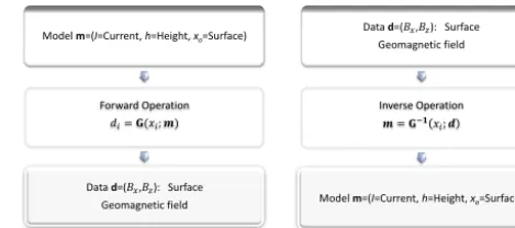
Figure 2. A sketch of the forward (left) and inverse (right) prob-lem. The residual is the difference between modelled and measured magnetic field:ri=di−G(xi;m)for theith data pointdi at sur-face positionxi. Sum of squared residuals over surface position is

S=6ir_i2for a least-squares inversion.Gis the objective function Eq. (1).

the exact quadratic step appropriate for a linear problem in a Gauss–Newton way. LM is adaptive because it controls its own damping. It raises damping if a step fails to reduce error. Otherwise, damping is reduced. In this way, the LM is capa-ble of alternating between a slow descent approach when far from the minimum and a fast convergence when in the neigh-bourhood of the minimum.

3.2.5 The computer software

The inversion set-up used in this study is an optimisa-tion curve-fitting tool in the Matlab programming language (MathWorks Inc., 2012) and the inversion problem is sum-marised in Table 1 and Fig. 2.

The Levenberg–Marquardt algorithm in Matlab terminates when at least one of the following conditions (exitflag value) is met:

4 Magnitude of search direction is smaller than the speci-fied tolerance.

3 Change in the residualwas less than the specified tol-erance.

2 Change inmwas less than the specified tolerance. 1 Function converged to a solutionm.

0 Number of iterations exceeded option “MaxIter”, or number of function evaluations exceeded option “Max-FunEvals”.

3.3 Inversion procedure

One needs a space domain over which the inversion must run. That is provided by the surface positionx, with a grid of data pointsdi=

dBx, dBz

T

(xi), 50 km apart from−1000 to +1000 km, wherexiis theith position of the datumdi along

the meridian. The frequency ω can also be a domain over which a different inversion problem could run. However, for purposes of this paper the period of the frequency is fixed to τ =2π/ω=5 min.

An objective function is the sum-of-squared residuals:

f(d, m)=X

i

[Fi(m)−di]2 (14)

=X

i

Bx Bz

(xi;m)−

dBx

dBz

(xi)

2

.

The model function is the ground geomagnetic field com-ponent expressions of Eq. (1). The comcom-ponents are complex valued and the code of the curve-fitting toolkit cannot oper-ate on complex values. Therefore, the model function should be expanded from the usual vector form

Bx, Bzto a matrix

ReBx,ReBz;ImBx,ImBzinstead. Here commas separate

columns and semi-colons separate rows. The geoelectric field on the ground, Eq. (2), remains in the forward problem. Once the set of output parameters are found by inversion, they can be substituted into Eq. (2) to estimate the geoelectric field.

Using the LM technique the objective function (sum-of-squared residuals) is minimised to determine the output pa-rameters of the model. In the LM, there are no equality or inequality restrictions, but bounds can be set for the parame-ters.

The aim of the inversion is to optimisef(d, m)to an in-put data setdof magnetic values reproduced here in the for-ward problem. Outputs are the parameter setmfrom any el-ements in the current system set [I, h, x0] and the layered Earth set [hn, σn] plusσN+1. In a full inversion, all the pa-rameters are adjusted simultaneously; otherwise, the inver-sion is partial with one or more parameters fixed and at least one parameter adjusted. For instance, adjusting only the cur-rent, when the other parameters do not take part, is a partial inversion. On the other hand, a full inversion adjusts all the parameters of both sets combined. Depending on the aims and scope of any geophysical research project that involves inversion theory, any combination of any number of param-eters from any set can be used in the optimisation (such as

m=[I, hn, σm];mn=1,2, . . .N ). In this study, however, we

will concern ourselves only with adjusting the current system set of parameters and fix the layered Earth set to the values of Quebec’s structure. Thus,m=[m1, m2, m3]=[I, h, x0].

From the placement of the current strengthI in the mag-netic field equations (Eq. 1), it is clear that the current strength is a linear model parameter, leading to a linear least-square inversion problem when only this parameter is adjusted. The current is unbounded and can even be zero

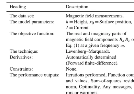
Table 1. Summary of the inversion set-up.

Heading Description

The data set: Magnetic field measurements. The model parameters: h=Height,x0=Surface position,

I=Current.

The objective function: The real and imaginary parts of magnetic field componentsBxBzof Eq. (1) at a given frequencyω. The technique: Levenberg–Marquardt. Derivatives: Automatically determined

(Forward finite-difference).

Constraints: None.

The performance outputs: Iterations performed, Function counts and values, Sum-of-squares residual norm, Optimality, Any messages, er-rors or warnings.

Table 2. Ground conductivity structure parameters for Quebec, Canada, [53◦450N, 71◦590W] (adapted from Boteler et al., 2000).

Layer Thickness (km) Conductivity (mS m−1)

Layer 1 15 0.05

Layer 2 10 5

Layer 3 125 1

Layer 4 200 10

Layer 5 ∞ 333

or negative. Placement of the height h and surface posi-tionx0 in those field expressions turns the inversion prob-lem into a nonlinear least-square fit. The surface position is also unbounded in both the negative and positive directions. The height can have no negative values however, hence the lower bound of 0 km (i.e. the surface). The skin depth and impedance are not output parameters to the inversion, as they are dependent on output parameters from the structure set. Since the structure set is fixed, these two surface quantities will be fixed when the period ofτ =5 min is fixed.

Optimisation results are shown in Sect. 5.

4 Preliminary work

The 1-D approximation of the ground conductivity struc-ture of Quebec, Canada, based on magneto-telluric measure-ments, is summarised in Table 2. Quebec appears to have a resistive structure. This can be used to calculate the material properties (skin depth and impedance) at the surface. This structure determines how the magnetic and electric fields be-have.

Table 3. Extreme values of the magnetic and electric field components at period τ=5 min obtained by using the ground conductivity structure of Quebec.

Bx(nT) Bz(nT) Ey(V km−1)

Complex parts ∼(1000+90i) ∼(−220+60i) ∼(−1.2−3.0i)

Amplitude and phase ∼(1004.04 at 5.14◦) ∼(228.04 at 164.74◦) ∼(3.23 at 248.20◦)

Geomagnetic and geoelectric fields

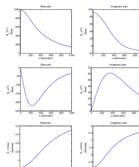
Once the impedance and skin depth were evaluated at the given period, one works out the respective electric and mag-netic fields (still in the forward problem, and shown in Fig. 3) of a line current with strength 1000 kA, positioned at xo=

0 km and a height of 300 km above the surface of the Earth. The extreme values obtained by reading off from the plots of Fig. 3 are listed in Table 3.

Thus, magnetic component Bx oscillates almost in phase

with fluctuations in the current, while componentBz is

al-most out of phase with the current (between 29.74 and 8.75◦ short of 180◦). The electric component Ey is more than

90◦behind the current (between 51.84 and 78.69◦ahead of 180◦).

Figure 3 gives a general idea of how the fields behave in the surface position space. These can be used in an inverse problem, for example to narrow down the region of interest and provide reasonable starting points for the search of the optimal point in parameter space.

5 Inversion results

Using the data reproduced in Fig. 3, an inversion was per-formed as a test to determine the parameters for the cur-rent system. This was done to make sure the inversion works properly and to check that the output parameters settle close to the expected values. The inversion worked no matter how far the parameters were initialised from their expected val-ues (as given in the caption of Fig. 3). The results of a full inversion are given in Fig. 4.

When all the parameters of a model are estimated in the in-version, that inversion is called a full inversion. When some parameters are fixed, that inversion is called a partial inver-sion. For partial inversions with either or both distance pa-rameters fixed, the distance papa-rameters have the constant val-ues given in the caption of Fig. 3. The parameter of the cur-rent was never fixed in all inversion cases. The fitted param-eters were initialised to the values given in the caption of Fig. 4.

Table 4 shows the final parameter values after the inver-sion in the three cases where the current and one or both dis-tance parameters were varied. The full inversion is “Case 1”, while the partial inversions are “Case 2” and “Case 3” re-spectively (with only one fixed parameter). All parameters are within 2 % below their values given in the caption of

0 200 400 600 800 1000

0 200 400 600 800 1000 Real part x (kilometer) Bx ( n T ) fi tt e d

0 200 400 600 800 1000

-20 0 20 40 60 80 100 Imaginary part x (kilometer) Bx ( n T ) fi tt e d

0 200 400 600 800 1000

-250 -200 -150 -100 -50 0 Real part x (kilometer) Bz ( n T ) fi tt e d

0 200 400 600 800 1000

0 10 20 30 40 50 60 70 Imaginary part x (kilometer) Bz ( n T ) fi tt e d

0 200 400 600 800 1000

-1.2 -1 -0.8 -0.6 -0.4 -0.2 Real part x (kilometer) Ey ( V /k m ) e s ti m a te

0 200 400 600 800 1000

-3 -2.5 -2 -1.5 -1 -0.5 0 Imaginary part x (kilometer) Ey ( V /k m ) e s ti m a te

Figure 3. Simulated magnetic (Bx, Bz) and electric (Ey) field com-ponent plots against surface position x in the forward problem (parameters:h=300 km,xo=0 km,I=103kA) for the Quebec structure and periodτ=5 min. Each complex part is plotted sep-arately. All plots are symmetric (Bx, Ey) or anti-symmetric (Bz) aroundx=0 km.

Fig. 3. Rerunning the inversion with both distance parame-ters fixed, thus varying only the current, produces the current strength atI =980±2.405 kA (or1I /I=0.245 %). This is not shown in Table 4; but it may be labelled as “Case 4”.

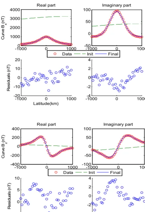
The residuals are not randomly distributed, as could be ex-pected from a Gaussian distribution of errors. The inversion is nevertheless a close to optimal fit of the model to the data. Inversion output parameter standard deviations, denoted by

Table 4. Deviations1mfrom the nominal valuesmof the inverted parameters in the form1m/m, from the inputs of the published data. The notation ofm∈ [I, h, xo]in each case is the parameter of interest.

Full inversion Current and height Current and latitude

(Case 1) (Case 2) (Case 3)

CurrentI[kA] 2.016/990.000 2.083/990.000 2.349/998.000 Heighth[km] 0.977/295.000 1.010/295.000 Fixed. Surfacexo[km] 0.972/1.620 Fixed. 1.144/1.590

-10000 0 1000

1000 2000 3000 4000 Real part C u rv e B x (n T )

Data Init Final

-1000 0 1000

-20 -10 0 10 20 Latitude(km) R e s id u a ls ( n T )

-1000 0 1000

-50 0 50 100

Imaginary part

Data Init Final

-1000-4 0 1000

-2 0 2 4

-1000 0 1000

-400 -200 0 200 400 Real part C u rv e B z (n T )

Data Init Final

-1000-5 0 1000

0 5 10 Latitude(km) R e s id u a ls ( n T )

-1000 0 1000

-100 -50 0 50 100 Imaginary part

Data Init Final

-1000-4 0 1000

-2 0 2 4

Figure 4. Fitted magnetic fieldsBx, Bzfrom inversion for the Que-bec ground conductivity structure at a period of τ=5 min. Ini-tial values of the parameters were as follows: current strengthI= 5×104kA, height h=6000 km, surface position xo=1000 km. Target parameter values were as follows:I=103kA,h=300 km andxo=0 km. A positive value ofxomeans a position north of the equator. All fitted parameters came close to their targeted values. The legends are defined as follows: “Data” is simulated magnetic field observations, “Init” is the initial estimate of the magnetic field before the inversion, “Final” is the final estimate of the magnetic field obtained through the inversion.

-1000 0 1000

-6000 -4000 -2000 0 Real part C u rv e E y (m V /k m )

Data Init Final

-1000 0 1000

-20 -10 0 10 Latitude(km) R e s id u a ls ( m V /k m )

-1000 0 1000

-10000 -5000 0

Imaginary part

Data Init Final

-1000 0 1000

-50 0 50 100

Figure 5. Estimated electric fieldEy from inversion of the simu-lated magnetic field data shown in Fig. 4 using the Quebec ground conductivity structure at a period ofτ=5 min. Initial values of the parameters were as follows: current strengthI=5×104kA, height

h=6000 km, surface positionxo=1000 km. Target parameter val-ues were as follows:I=103kA,h=300 km and xo=0 km. A positive value ofxomeans a position north of the equator. All fitted parameters came close to their target values. The legends are de-fined as follows: “Data” is electric field simulations from simulated magnetic field observations viaEy(xi, ω)= −Z(ω)Hx(xi, ω)(see Fig. 1), “Init” is the initial estimate of the electric field before the in-version (using parameter initial values), “Final” is the final estimate of the electric field obtained after the inversion (using parameter final values obtained by the inversion).

6 Conclusions

This paper demonstrates the use of inversion techniques, us-ing the complex image method to determine the parameters (current strength and/or two positions) of the line current by fitting the ionospheric currents to magnetic data calculated from Eq. (1). For this purpose the ionospheric current was taken as a line current above the Earth. No field-aligned cur-rents were considered.

1 % below target. Case 4 is the worst case: the current is 2 % below target.

The value of the estimated current height decreases by 35 km when the surface position is fixed (in both Cases 1 and 2) and gets closer to a target value of 300 km. The value of the estimated surface position moves south to within 2 km of the target at the equator, when the height is fixed, but not crossing the equator (in Cases 1 and 3 respectively).

Appendix A

A1 Magnetotelluric basics

We start with Faraday’s law of induction, which describes the relationship between the magnetic and electric field: ∇ ×E= −∂B

∂t . (A1)

Variations in the horizontal magnetic field components Bx

andBy induce a geoelectric field which then drives an

elec-tric current in the Earth according to Ohm’s lawJ=σ E. The geoelectric field at the Earth’s surface can be modelled using the plane wave model (Viljanen and Pirjola, 1989; Pirjola, 2002).

A2 Homogeneous Earth model

As a first approximation, we assume the Earth is a uni-form half-space of homogeneous conductivity and assume that there is a plane wave field that propagates vertically downwards. Using a Cartesian coordinate system where the xy plane corresponds to the Earth’s surface, then at a single frequencyωthe fields of a plane wave can be expressed as

E(x, t )=Eoei(ωt−kz)orB(x, t )=Boei(ωt−kz), (A2)

whereEo=(ExEyEz)andBo=(BxByBz).

For the given frequencyω, the propagation constantk is given byk= −iκ, whereκ=ω√εoµo. For a lossy medium

the skin depth is complex. For a good conductor and low frequencies the quasi-static approximation (ωεo/σ1)can

be applied: 1

p =

p

iωµoσ

p

1+iωεo/σ≈

p

iωµoσ=

1+i

δ , (A3)

whereµoandεo are the permeability and permittivity

con-stants of free space andσ the uniform conductivity. Here use was made of a complex identity

√

i=(1+i) / √

2.

In a homogeneous conducting medium with uniform con-ductivity, the plane wave amplitude decays with depth into the medium. The depth at which the amplitude has decayed toe−1 times the amplitude at the surface is the skin depth δ=√2/ωµoσ. And the complex skin depth isp.

It can be shown thatκδ=√2ωεo/σ. The approximation

of the reflection coefficient by an exponential function is based on the assumption κδ1. This assumption is justi-fied in the context of GIC modelling since the spectrum of the geomagnetic field is typically in the range 1 to 10 mHz. For a homogeneous ground conductivity of σ=1 mS m−1, which is typical for the locations of interest, the values ofδκ are in the range 10−6to 10−5.

With Eq. (A2) substituted into Eq. (A1) it follows that the ratios between the orthogonal electric and magnetic field components define the surface impedance Z(ω). The ratio

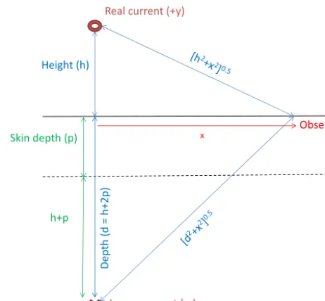
Height (h)

Skin depth (p) x

h+p

Real current (+y)

Image current (-y)

Observer

D

e

p

th

(

d

=

h

+

2

p

)

Figure A1. Plane-Earth model of the current image method for a 1-D representation of a conductivity structure. Labels define the con-cepts of the method.

between the electric field and the spectral component atωof the time derivative of the magnetic field, ∂_∂tB, which will be denoted byB˙ (referred to as B-dot) defines the complex skin depthp(Deri et al., 1981). Thus,

Ex By

= −Ey Bx

=Z (ω) µo

= 1

µo

r

µoω

iσ and (A4)

Ex ˙ By

= −Ey ˙ Bx

=Z (ω) iωµo

= 1

i√iµoωσ

= −ip.

A3 Elementary fields

From Maxwell’s equations in the plane-Earth model (Fig. A1) and the quasi-static approximation, a diffusion equation is derived and an electric field elementary solu-tion is found (Hermance and Peltier, 1970) – i.e.∇2Ey= iωσ µoEy, with Ey(x, z;ω, ν)=e±γ zcosνx where γ2= ν2+iωσ µoin Cartesian coordinates.

There are however both incidente−γ zand reflectede+γ z waves; the solution is symmetrical inx aroundx=0, and above the Earth’s surface (z >0)γ =νbecauseσ=0 there. Thus, the electric field is given by

Ey(x, z;ω, ν)=C e−νz−Reνzcosνx, (A5a)

whereR(ω)is the reflection coefficient andCis an arbitrary constant.

are

Hx(x, z;ω, ν)= −C ν iωµ e

−νz_+Reνz

cosνx (A5b) Hz(x, z;ω, ν)=C

ν iωµ e

−νz_−Reνz

sinνx. (A5c) A4 Layered-Earth model

We next consider a multi-layered model of the Earth. The appendix of Wait (1980) described a general approach to de-termineZ(ω)from the 1-D multilayer ground conductivity structure of a given location. We assume N planar layers in the ground below the Earth’s surface. Each layer (n= N, . . .,1)has a finite thicknesshnand a uniform

conductiv-ityσn. Correspondingly, uniform elementary impedances can

be obtained from the conductivity for each layer. We define a modified wave number for each layer κn. Equation (A3)

still applies, but theµo,εoandσare replaced byµn,εnand σnrespectively for each layer. The intrinsic layer impedance

is defined byKn=iωµn/κn and related to the layer

reflec-tion by Rn=K_Kn_n−+ZZnn. For a good conductor in quasi-static

approximation (ωεn/σn1), we haveκn= √

iωµnσn and Kn=

√

iωµn/σn.

The(N+1)th layer is called the remaining half-space in plane-Earth geometry and is assumed to have infinite thick-ness, uniform conductivityσN+1and layer impedanceKN+1. These layer impedances are independent of each other. To re-late them, a second set of impedancesZn at the boundaries

are defined which are dependent on the layer thicknesses and layer impedances of the layers below and up to that bound-ary. For the lowest boundary, separating the half-space from the next layer, the boundary impedance is ZN+1=KN+1.

Thus, a recursion relation is set up, starting at the bottom and working all the way up to the top (that is forn=N, . . .,1): Zn=Kn

Zn+1−Kntanhνnhn Kn−Zn+1tanhνnhn

. (A6)

Then the surface impedance is the boundary impedance of the Earth’s surface:Z(ω)=Z1. In general, the constants of permittivityεnand permeabilityµnare all different for each

layer. In the present study the layer permittivities are all set toεn=ε0and the layer permeabilities toµn=µ0for alln. A5 Complex image method

Next, we consider the complex image method (CIM) and an approximation to the reflection coefficient to accommo-date this method. For convenience, this also introduces an equally important material property called the skin depth for multi-layered Earth. The other important material property is the surface impedance. The surface skin depth is computed from the surface impedance as p(ω)=Z(ω)/ iωµ0. How-ever, the surface is a boundary of the layered-Earth model and, as with boundary impedances Zn, one can also form

a set of boundary skin depths pn similarly computed from

these impedances (withµnreplacingµ0).

The reflection coefficient (Boteler and Pirjola, 1998) can be expressed as

R (Z;ω, ν)=K−Z K+Z =

iωµ0/ν−Z iωµ0/ν+Z

(A7) =iωµ0−νZ

iωµ0+νZ

=1−νp 1+νp.

Note thatR depends not only on angular frequencyω and wave numberν, but also on the complex surface impedance Z(ω)or skin depthp(ω).

Under the condition that pν1, it can be shown that the reflection coefficient can be written in exponential form which facilitates analytic solution of the inversion integrals. Replace the Taylor expansion of Eq. (A7) with the Taylor expansion of an exponential function; then,R≈e−2pν. This can then be inserted into the Fourier integral expressions for the magnetic and electric fields, which then makes it possible to derive their solutions analytically.

Here the image current is employed to represent the re-flected part of the electromagnetic field off the Earth’s sur-face (or equivalently a layered conductive Earth). An image line current is assumed to be flowing in the opposite direction to the external line current at a depthz=h+2p.

A6 Geomagnetic and geoelectric fields in a plane-Earth model

To relate the elementary fields (in Sect. A3) to that of a line current, one must take Fourier integrals of the components over propagation spaceν. This forms the total fields over surface distance and frequency space at the Earth’s surface (z=0). Adapted from Boteler et al. (2000), the geoelectric and geomagnetic field components are then





Ey Bx Bz



(x, ω)= 



Ey µHx µHz



(x, ω) (A8)

= µ

2π ∞

Z

0 J (ν)





iω (R−1)cos(νx) ν−1 (R+1)cos(νx) (R−1)sin(νx)



e

−νh_dν,

where J (ν)=R_−∞∞ j (x) e−iνxdx is the current density. These integrals look like a Fourier transform of the integral in Biot–Savart’s law in thexν-space.

Boteler et al. (2000) discuss distributions of currents of one type and points out a field equivalence. For a current system defined by a Cauchy distribution, characterised by a spread parametera, we havej (x)= I

π a

a2_+x2 and the

would be equivalent to those created by a line current sys-tem placed at a height ofz= −(h+a). The new height can be denoted as z= −h0. Cauchy distributed current systems are represented by line currents further from the z=0 in-terface (the Earth’s surface), as determined by the Cauchy parameter. Therefore, one can disregard the need for such distributions, and consider only line current systems. A line current would only have j (x)=I δ (x), leading to J (ν)= IR_−∞∞ δ (x) e−iνxdx=I.

The integrals will need to be solved numerically if the ex-act expression for R in Eq. (A7) is substituted for the re-flection coefficient. No closed analytic solutions exist for the combination of elementary functions present in the resulting integrands. However, replacing the reflection coefficient in the integrals by its approximation to Eq. (A7) means there will only be two elementary functions in the integrands: the trigonometric and exponential functions. Exact solutions for

these types of integrals have been derived, and that serves as a motivation for using the image current method in simplify-ing the derivation and evaluation of these integrals. Maksimplify-ing all the substitutions to Eq. (A8), the final form solutions can be obtained from any standard integral table, and is given as





Ey Bx Bz



(x, ω) (A9)

=µI 2π

∞

Z

0





iω e−2pν−1cos(νx) ν−1 e−2pν+1

cos(νx) e−2pν−1sin(νx)



e

−νh_dν

=µI 2π



  

iω

2 ln

h2+x2 (h+2p)2+x2

h+2p (h+2p)2+x2+

h h2_+x2 x

(h+2p)2+x2− x h2_+x2



Acknowledgements. The results presented in this paper rely on the

data collected at SANSA Space Science Directorate (formerly the Hermanus Magnetic Observatory). We thank the South African Na-tional Space Agency (SANSA) for supporting its operation and IN-TERMAGNET for promoting high standards of magnetic observa-tory practice (www.intermagnet.org).

Topical Editor H. Kil thanks D. Danskin and one anonymous referee for their help in evaluating this paper.

References

Albertson, V. D., Bozoki, B., Feero, W. E., Kappenman, J. G., Larsen, E. V., Nordell, D. E., Ponder, J., Prabhakara, F. S., Thompson, K., and Walling, R.: Geomagnetic disturbance effects on power systems, IEEE T. Power Deliver., 8, 1206–1216, 1993. Boteler, D. H. and Pirjola, R. J.: The complex-image method for calculating the electric and magnetic fields produced at the sur-face of the Earth by the auroral electrojet, Geophys. J. Int., 132, 31–40, 1998.

Boteler, D. H., Pirjola, R. J., and Trichtchenko, L.: On calculating the electrical and magnetic fields produced in technological sys-tems at the Earth’s surface by a “wide” electrojet, J. Atmos. Sol.-Terr. Phy., 62, 1311–1315, 2000.

Chave, A. D. and Jones, A. G.: The magnetotelluric method: theory and practice, Cambridge University Press, 2012.

Dearholt, D. W. and McSpadden, W. R.: Electromagnetic wave propagation, McGraw-Hill Incorporated, 1973.

Deri, A., Tevan, G., Semlyen, A., and Castanheira, A.: The complex ground return plane, a simplified model for homogeneous and multi-layer earth return, IEEE T. Power App. Syst., PAS-100, 3686–3693, 1981.

Hadamard, J.: Sur les problemes aux derivees partielles et leur signi-fication physique (English: On problems with partial derivatives and their physical meaning), Princeton Univesrity Bulletin, 49– 52, 1902.

Hakkinen, L. and Pirjola, R.: Calculation of electric and magnetic fields due to an electrojet current system above a layered Earth, Geophysica, 22.1–2, 31–44, 1986.

Hermance, J. F. and Peltier, W. R.: Magnetotelluric fields of a line current, J. Geophys. Res., 75, 3351–3356, 1970.

INTERMAGNET: available at: www.intermagnet.org/publications/ IM_ESTEC.pdf, last access: 7 July 2014.

Kerridge, D.: INTERMAGNET: Worldwide near-real-time geo-magnetic observatory data, in: Proceedings of the Workshop on Space Weather, ESTEC, 34, December 2001.

Lourakis, M. I. A.: A brief description of the Levenberg-Marquardt algorithm implemented by Levmar, Institute of Computer Sci-ence, Foundation for Research and Technology, Hellas, Greece, 2005.

MathWorks Inc.: Optimization theory overview, avail-able at: http://www.mathworks.com/help/optim/ug/ optimization-theory-overview.html (last access: 30 Octo-ber 2013), 2012.

Pirjola, R.: Geomagnetic effects on ground-based technological sys-tems, Surv. Geophys., 23, 71–90, 2002.

Pirjola, R. and Viljanen, A.: Complex image method for cal-culating electric and magnetic fields produced by an auro-ral electrojet of finite length, Ann. Geophys., 16, 1434–1444, doi:10.1007/s00585-998-1434-6, 1998.

Shea, M. A. and Smart, D. F.: Overview of the effects of solar-terrestrial phenomena on man and its environment, Il Nuovo Ci-mento, 19, 945–952, 1996.

Tarantola, A.: Inverse problem theory, Society of Industrial and Ap-plied Mathematics (SIAM), Philadelphia, 2005.

Thomson, D. J. and Weaver, J. T.: The complex image approxima-tion for inducapproxima-tion in a multilayered Earth, J. Geophys. Res., 80.1, 123–129, 1975.

Viljanen, A. and Pirjola, R.: Statistics on geomagnetically-induced currents in the Finnish 400 kV power system based on recordings of geomagnetic variations, J. Geomagn. Geoelectr., 41, 411–420, 1989.

Wait, J. R.: Electromagnetic surface impedance for a layered earth for excitation, Radio Sci., 15.1, 129–134, 1980.

Wait, J. R. and Spies, K. P.: On the representation of the quasi-static fields of a line current source above the ground, Can. J. Phys., 47, 2731–2733, 1969.

Wilkinson, P.: Book review: Space weather: Physics and effects, Space Weather, 5, S11007, doi:10.1029/2007SW000334, 2007. Withbroe, G. L.: Living With a Star, in: Space Weather, edited by: