Influence of infrastructure on water quality and greenhouse gas dynamics in urban streams

https://doi.org/10.5194/bg-14-2831-2017 © Author(s) 2017. This work is distributed under the Creative Commons Attribution 3.0 License.

Influence of infrastructure on water quality and greenhouse gas

dynamics in urban streams

Rose M. Smith1,2, Sujay S. Kaushal2, Jake J. Beaulieu3, Michael J. Pennino4,5, and Claire Welty5

1_{Department of Biology, University of Utah, Salt Lake City, UT 84112, USA}

2_{Department of Geology, Earth System Science Interdisciplinary Center, University of Maryland,}

College Park, MD 20742, USA

3_{US Environmental Protection Agency, Office of Research and Development, National Risk}

Management Research Laboratory, Cincinnati, OH 45220, USA

4_{US Environmental Protection Agency National Health and Environmental Effects Research Lab,}

Corvallis, OR 97333, USA

5_{Department of Chemical, Biochemical, and Environmental Engineering, Center for Urban}

Environmental Research and Education, University of Maryland Baltimore County, Baltimore, MD 21250, USA

Correspondence to:Rose M. Smith (smithrose24@gmail.com)

Received: 8 September 2016 – Discussion started: 15 September 2016

Revised: 11 March 2017 – Accepted: 18 April 2017 – Published: 13 June 2017

Abstract. Streams and rivers are significant sources of ni-trous oxide (N2O), carbon dioxide (CO2), and methane

(CH4)globally, and watershed management can alter

green-house gas (GHG) emissions from streams. We hypothesized that urban infrastructure significantly alters downstream wa-ter quality and contributes to variability in GHG satura-tion and emissions. We measured gas saturasatura-tion and esti-mated emission rates in headwaters of two urban stream net-works (Red Run and Dead Run) of the Baltimore Ecosys-tem Study Long-Term Ecological Research project. We iden-tified four combinations of stormwater and sanitary infras-tructure present in these watersheds, including: (1) stream burial, (2) inline stormwater wetlands, (3) riparian/floodplain preservation, and (4) septic systems. We selected two first-order catchments in each of these categories and measured GHG concentrations, emissions, and dissolved inorganic and organic carbon (DIC and DOC) and nutrient concentrations biweekly for 1 year. From a water quality perspective, the DOC : NO−₃ ratio of streamwater was significantly differ-ent across infrastructure categories. Multiple linear regres-sions including DOC : NO−₃ and other variables (dissolved oxygen, DO; total dissolved nitrogen, TDN; and tempera-ture) explained much of the statistical variation in nitrous oxide (N2O, r2=0.78), carbon dioxide (CO2, r2=0.78),

and methane (CH4,r2=0.50) saturation in stream water. We

measured N2O saturation ratios, which were among the

high-est reported in the literature for streams, ranging from 1.1 to 47 across all sites and dates. N2O saturation ratios were

highest in streams draining watersheds with septic systems and strongly correlated with TDN. The CO2saturation ratio

was highly correlated with the N2O saturation ratio across all

sites and dates, and the CO2saturation ratio ranged from 1.1

to 73. CH4was always supersaturated, with saturation ratios

ranging from 3.0 to 2157. Longitudinal surveys extending form headwaters to third-order outlets of Red Run and Dead Run took place in spring and fall. Linear regressions of these data yielded significant negative relationships between each gas with increasing watershed size as well as consistent re-lationships between solutes (TDN or DOC, and DOC : TDN ratio) and gas saturation. Despite a decline in gas saturation between the headwaters and stream outlet, streams remained saturated with GHGs throughout the drainage network, sug-gesting that urban streams are continuous sources of CO2,

CH4, and N2O. Our results suggest that infrastructure

1 Introduction

Streams and rivers are dynamic networks that emit glob-ally significant quantities of carbon dioxide (CO2), methane

(CH4), and nitrous oxide (N2O) to the atmosphere. CO2

emissions via flowing waters are equivalent to half of the annual terrestrial carbon sink (1.2 Pg CO2-C yr−1, Cole et

al., 2007; Battin et al., 2008). Stanley et al. (2016) re-cently demonstrated that flowing waters are significant CH4

sources as well, emitting approximately 28 Tg yr−1, which is equivalent to between 10 and 35 % of emissions from wet-lands globally (Bridgham et al., 2013). Approximately 10 % of global anthropogenic N2O emissions are emitted from

river networks due to nitrogen contamination of surface and groundwater (UNEP, 2013; Ciais et al., 2013). There is evi-dence that these N2O estimates, based on IPCC guidelines,

might be too low, given growing evidence of high denitrifi-cation rates in small streams with high NO−₃ loads (Beaulieu et al., 2011).

While much of the research on greenhouse gas (GHG) emissions from streams has taken place in agricultural water-sheds, urban-impacted river networks receive similar N loads and have also shown elevated GHG concentrations and emis-sions (e.g., Daniel et al., 2001; Beaulieu et al., 2010, 2011; Kaushal et al., 2014a; Gallo et al., 2014). As urban land cover and populations continue to expand, it is critical to under-stand the impacts on downstream waters, including C and N loading and GHG emissions. While N2O emissions from

both urban and agricultural sources are taken into account in models based on estimated watershed dissolved inorganic ni-trogen loading (Nevison et al., 2000; Seitzinger et al., 2000), measurements validating these estimates or estimates of CO2

and CH4in urban watersheds are rare. Quantifying the

vari-ability, drivers, and sources of GHG emissions from streams will illuminate the biogeochemical processes and potential role of urban infrastructure on nutrient cycling, water qual-ity, and GHG budgets.

1.1 Role of sanitary infrastructure

The form and age of stormwater and sanitary infrastructure within a watershed can influence stream water GHG emis-sions in several ways. GHGs may enter urban streams di-rectly through buried stormwater and sanitary infrastructure or form increased production within streams in response to nutrient loading and/or geomorphic changes. We investigated the role of infrastructure on GHG emissions from streams in order to evaluate these potential drivers of heterogene-ity within urban watersheds. Sanitary infrastructure encom-passes a wide array of systems to manage human waste. In developed countries, sanitary infrastructure includes a com-bination of septic systems, sanitary sewers, and sometimes combined stormwater and sanitary sewers. Storm and sani-tary sewer lines are present in areas with medium-to-high-density development. The sanitary sewer or combined sewer

network delivers waste to centralized wastewater treatment plants (WWTPs), which treat influent and release effluent into larger rivers or coastal zones. Sanitary, storm, and com-bined sewers tend to follow stream valleys (i.e., low points in the landscape), are often made of erodible materials such as terra cotta or concrete, and tend to crack or develop leaks. Leaks in sanitary sewer infrastructure can lead to chronic nutrient loading throughout stream networks (Divers et al., 2013, Kaushal et al., 2011, 2015; Pennino et al., 2016). Sep-tic systems, primarily used in low-density residential areas, are designed to settle out waste solids and leach N-rich liquid waste into subsurface soils and groundwater. Sanitary sewer infrastructure may influence GHG abundance and emission from streams directly via diffusion of gases out of gravity sewer lines (Short et al., 2014) or indirectly by microbial processing along surface and subsurface flow paths (Yu et al., 2013; Beaulieu et al., 2011). While the present study fo-cuses mainly on first- to third-order streams influenced by sanitary sewer lines or septic systems, it is also worth men-tioning that WWTPs are known to be a source of CH4 and

N2O in urban areas and contribute point-source GHG

load-ing to larger rivers and coastal areas (Beaulieu et al., 2010; Strokal and Kroeze, 2014; Alshboul et al., 2016).

Sewage leaks are likely the primary source of N2O

emis-sions from small urban streams (Short et al., 2014). Sev-eral studies have documented that wastewater leakage from municipal sewers often accounts for more than 50 % of dis-solved N in urban streams (Kaushal et al., 2011; Pennino et al., 2016; Divers et al., 2013). While sanitary sewer lines are known to leak dissolved N, N2O losses are not accounted for

in greenhouse gas budgets of the large WWTPs that these pipes feed into. Short et al. (2014) measured intake lines from three municipal WWTPs and estimated that N2O

emis-sions from sewer lines alone are on the same order of mag-nitude (1.7 g N2O person yr−1)as current IPCC estimates for

per capita emissions from secondary WWTPs. Their study demonstrates the importance of constraining biogenic gas emissions from streams, which flow alongside and may re-ceive gaseous inputs from aging sanitary sewer lines. 1.2 Role of stormwater infrastructure

within 100 m of the stream corridor for new developments (Baltimore Department of planning, 2010).

The form of stormwater infrastructure – whether stream burial, infiltration wetland, or restored riparian zone – may contribute to GHG saturation of groundwater and streams. Stormwater control wetlands and riparian/floodplain preser-vation may increase or decrease CH4 and N2O emissions

from streams, depending upon how watershed C and N in-puts are routed along hydro-biogeochemical flow paths. For instance, if these forms of GI are successful at removing excess N inputs to streams, GI may reduce N2O emissions

from flowing waters. Alternatively, GI may increase both N2O and CH4inputs to streams and thus emissions by

facil-itating anaerobic microbial metabolism (Søvik et al., 2006; VanderZaag et al., 2010). The form of GI (i.e., stormwa-ter control wetland vs. riparian/floodplain preservation) may also influence GHGs due to (1) differences in water residence time and oxygen depletion in wetland vs. floodplain soils and (2) differences in watershed-scale N removal capacity of the two different approaches.

1.3 Variables controlling GHG production in urban watersheds

Reach-scale studies in streams across biomes have demon-strated that GHG production and emission is sensitive to changes in nutrient stoichiometry, organic matter quality, re-dox state, and temperature (e.g., Bernot et al., 2010; Kaushal et al., 2014a; Beaulieu et al., 2009; Dinsmore et al., 2009; Baulch et al., 2011; Harrison and Matson, 2003). Several studies have shown that infrastructure can influence so-lute loading and stoichiometry of streams, which could in turn increase GHG production. For instance, Newcomer et al. (2012) measured higher rates of N uptake and denitrifi-cation potential in streams with restored riparian zones com-pared with degraded, incised urban streams. In-stream N up-take is also consistently higher in daylighted streams com-pared with streams buried in pipes (Pennino et al., 2014; Beaulieu et al., 2015). Upland or inline stormwater wetlands and retention ponds provide additional locations for focused N removal in urban watersheds (Newcomer Johnson et al., 2014; Bettez and Groffman, 2012). Sanitary infrastructure (i.e., leaky sewer lines and septic systems) can also be a source of N via leaching into groundwater (Shields et al., 2008; Kaushal et al., 2015; Pennino et al., 2016).

In previous studies, carbon quantity and/or organic mat-ter quality was correlated with N uptake or removal in ur-ban streams and wetlands (Newcomer et al., 2012; Pen-nino et al., 2014; Beaulieu et al., 2015; Bettez and Groff-man, 2012; Kaushal et al., 2014c). Inverse relationships be-tween dissolved organic carbon (DOC) and nitrate (NO−₃) concentrations have been found to persist across a wide va-riety of ecosystems ranging from soils to streams to oceans (e.g., Aitkenhead-Peterson and McDowell, 2000; Dodds et al., 2004; Kaushal and Lewis, 2005; Taylor and Townsend,

2010). Recently, inverse relationships between DOC and NO−₃ have also been reported for urban environments rang-ing from groundwater to streams to river networks (Mayer et al., 2010; Kaushal and Belt, 2012; Kaushal et al., 2014c). A suite of competing biotic processes may control this re-lationship, by either (1) assimilating or reducing NO−₃ in the presence of bioavailable DOC or (2) by producing NO−₃ regardless of DOC status (Hedin et al., 1998; Dodds et al., 2004; Kaushal and Lewis, 2005; Taylor and Townsend, 2010). The former category includes heterotrophic denitrifi-cation, which oxidizes organic carbon to CO2and reduces

NO−₃ to N2O+N2(Knowles, 1982) as well as assimilation

of inorganic N (Wymore et al., 2015; Caraco et al., 1998; Kaushal and Lewis, 2005). In the second category, nitri-fication chemoautotrophically produces NO−₃ by oxidizing NH+₄ and consuming CO2. Nitrification also yields N2O as

an intermediate product and has been shown to dominate N cycling processes in low-DOC environments (Schlesinger, 1997; Taylor and Townsend, 2010; Helton et al., 2015).

In urban watersheds, denitrification is often limited by DOC due to increased N loading and/or decreased connec-tivity with carbon-rich soils in the riparian zone (Mayer et al., 2010; Newcomer et al., 2012). The C : N stoichiometry is likely to be affected by stormwater and sanitary sewer in-frastructure designs as well (Søvik et al., 2006; Collins et al., 2010; Kaushal et al., 2011). Stormwater wetlands may promote anoxic conditions and increase the C : N ratio of stream water by increasing flow through carbon-rich soils (e.g., Søvik et al., 2006; Newcomer et al., 2012). Stream burial can reduce C : N ratios, if streams are buried in storm drains (Pennino et al., 2016; Beaulieu et al., 2014). Leaky sanitary infrastructure may additionally reduce the C : N ra-tio and/or alter the form of carbon in streams (Newcomer et al., 2012).

1.4 Study goals

Figure 1.Site map of headwater stream sites within Red Run and Dead Run watersheds. Green stars signify biweekly sampling sites, and black dots signify longitudinal sampling points sampled seasonally. Land cover categories are colored based on the National Land Cover Database, with dark red areas signifying dense urban land cover, light red signifying medium urban land cover, and green colors signifying forested or undeveloped areas. Close-up views of Dead Run and Red Run on the right represent the study watersheds.

understanding of the relationship between infrastructure type and biogeochemical functions is critical for minimizing un-intended consequences of water quality management, espe-cially as growing urban populations place greater burden on watershed infrastructure (Doyle et al., 2008; Foley et al., 2005; Strokal and Kroeze, 2014).

1.5 Sampling methods 1.5.1 Study sites

This study took place in collaboration with the Baltimore Ecosystem Study Long-Term Ecological Research project (www.beslter.org). We identified four categories based on distinct combinations of stormwater and sanitary infrastruc-ture dominating the greater Baltimore region, based on maps of stormwater control structures, housing age, and inten-sive field surveys. We then selected eight first-order streams paired across the four categories. First-order stream sites were spread equally across two sub-watersheds of Gwynns Falls: Dead Run and Read Run (Fig. 1). We have abbreviated the categories based on the dominant infrastructure feature as follows: (1) stream burial, (2) inline stormwater management wetlands, (3) riparian/floodplain preservation, and (4) septic systems (Table 1).

Sites in the “stream burial” category (DRAL and DIRS) drain watersheds with streams contained in storm sewers. Sanitary infrastructure in these watersheds is composed of aged sanitary sewer lines, installed prior to 1970 (Balti-more County Department of Planning, 2010). Streams in

the “inline stormwater management” category (DRKV and DRGG) originate in stormwater ponds or wetlands and also flow adjacent to aging sanitary sewer lines. Streams in the “riparian/floodplain preservation” category (RRRM and RRSM) drain watersheds with newer development (after 2000), upland infiltration wetlands, and 100 m wide unde-veloped floodplains (Baltimore County Department of Plan-ning, 2010). Sanitary sewers were constructed in these wa-tersheds between 2000 and 2010 (Baltimore County De-partment of Planning, 2010). Sites in the “septic systems” category (RRSM and RRSD) drain lower density develop-ment with stormwater managedevelop-ment in the form of stormwa-ter sewer pipes (Fig. 1). All eight first-order stream sites were sampled every 2 weeks for dissolved carbon and nitrogen concentrations.

1.5.2 Temporal sampling of dissolved gases and stream chemistry

Headwater stream sites were sampled every 2 weeks for so-lutes (DOC; total dissolved nitrogen, TDN; humification in-dex, HIX; and biological autochthonous inputs inin-dex, BIX) and dissolved gas (CO2, CH4 and N2O) concentrations.

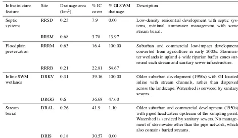
Table 1.Summary of site characteristics including drainage area (km2), percent impervious cover (%IC), and percent of the watershed drained by GI stormwater best management practices (i %GI SWM drainage).

Infrastructure Site Drainage area % IC % GI SWM Description

feature (km2) cover drainage

Septic systems

RRSD 0.23 7.9 0.00 Low-density residential development with septic sys-tems, minimal stormwater management with some stream burial.

RRSM 0.68 3.78 13.97

Floodplain preservation

RRRM 0.63 16.4 100.00 Suburban and commercial low-impact development converted from agriculture in early 2000s. Stormwa-ter wetlands in upland+wide riparian buffer zones sur-round each stream and sanitary sewer infrastructure.

RRRB 0.21 22.81 54.67

Inline SWM wetlands

DRKV 0.31 39.16 100.00 Older suburban development (1950s) with GI located inline with stream channels, rather than dispersed across the landscape. Watershed is serviced by sanitary sewers.

DRGG 0.6 36.68 47.60

Stream burial

DRAL 0.26 41.9 1.10 Older suburban and commercial development (1950s) with piped headwaters upstream of the sampling point. Watershed is serviced by sanitary sewers. No manage-ment of stormwater other than the pipe network, which also contains buried streams.

DRIS 0.18 30.57 0.00

from the fixed starting point of the study reach. Samples were collected by submerging a 140 mL syringe with a three-way Luer lock and pulling 115 mL of stream water into the sy-ringe. We added 25 mL of ultra-high purity helium to the syringe in the field and then shook the syringes vigorously for 5 min to promote equilibration of gases between aqueous and gas phases. After equilibration, 20 mL of the headspace was immediately transferred into a pre-evacuated glass vial capped with a screw-top rubber septum (LabCo Limited, Lampeter, UK) and then transported to the laboratory, where samples were stored at room temperature for up to 4 weeks prior to analyses. Water temperature and barometric pressure during the equilibration were recorded in the field. We col-lected three helium headspace blanks by injecting 25 mL of helium into pre-evacuated vials in the field.

We collected stream water samples in a 250 mL high-density polyethylene bottles, one sample per site. One dupli-cate sample was collected on each sampling date, and the site for duplicate sample collection rotated among the sampling dates. Dissolved oxygen (DO) concentration and pH were measured at the upstream end of each study reach using a handheld YSI 550-A dissolved oxygen meter (YSI Inc., Yel-low Springs, OH) and an Oakton handheld pH meter (Oakton Instruments, Vernon Hills, IL).

1.5.3 Longitudinal sampling of dissolved gases

Longitudinal surveys were conducted in June 2012, March 2014, and December 2014 in Red Run and Dead Run. Longitudinal sampling started at the outlet of each ma-jor tributary (Dead Run or Red Run) and extended every 500 m upstream to include the four biweekly sampled head-water sites in each head-watershed (Fig. 1). During spring and fall months, solute and gas samples were collected along all major tributaries (> 5 % main stem flow) as well as ev-ery 500 m along the main stem of Dead Run and Red Run. Minor tributaries (< 5 % of main stem flow) were not sam-pled. Stream discharge was measured at each sampling point using a Marsh-McBirney Flo-Mate handheld velocity me-ter (Marsh-McBirney Inc., Frederick, MD, USA). We used cross-sectional measurements of stream velocity and wa-ter depth to calculate instantaneous discharge at each sam-pling site. We measured velocity and depth at a minimum of 10 points at each cross section in order to properly charac-terize flow across the channel. Discharge data were provided by USGS when sampling sites were co-located with a USGS gaging station (US Geological Survey, 2017).

were always co-located with road crossings, we were able to acquire the latitude and longitude of sampling sites using Google Earth software (Google Inc., 2009). Watersheds were delineated using a 2 m resolution digital elevation model (DEM; Baltimore County Government, 2002). We first cor-rected the DEM for spurious depressions using the “Fill” tool in the ArcMap10.0 Hydrology toolbox. Next, we calcu-lated flow direction for each pixel of this filled DEM raster. We then used the “Flow Accumulation” tool to evaluate the number of pixels contributing to each downstream pixel. Af-ter ensuring that each pour point was co-located on the map streams (i.e., areas with flow accumulation > 500 pixels), we used the “Watershed” tool to delineate the pixels draining into each sampled location.

1.6 Laboratory methods

1.6.1 Dissolved gas concentrations

Samples of headspace equilibrated gas concentrations (CO2,

CH4, and N2O) were stored at room temperature for up to

1 month in airtight exetainer vials and transported to the EPA National Risk Management Research Laboratory, Cincinnati, Ohio, for analysis. Concentrations of CO2, CH4, and N2O

were measured using a Bruker 450 (Bruker, Billerica, MA, USA) gas chromatograph equipped with a methanizer, flame ionization detector, and electron capture detector. Instrument detection limits were 100 ppb for N2O, 10 ppm for CO2, and

0.1 ppm for CH4.

1.6.2 Solute concentrations

Water samples were transported on ice to the University of Maryland, College Park, and filtered using pre-combusted 0.7 µm glass fiber filters within 24 h. A Shimadzu TOC ana-lyzer (Shimadzu Scientific, Kyoto, Japan) was used to mea-sure total dissolved nitrogen and dissolved organic carbon. The non-purgeable organic carbon (NPOC) method was uti-lized for DOC, despite potential underestimation of volatile compounds because the NPOC method is insensitive to vari-ations in dissolved inorganic carbon (DIC; Findlay et al., 2010). TDN was measured on the same instrument using the “TDN” method, which consists of high-temperature combus-tion in the presence of a platinum catalyst. Nitrate (NO−₃) concentrations were measured via colorimetric reaction us-ing a cadmium reduction column (Lachat method 10-107-04-1-A) on a Lachat flow injection analyzer (Hach, Love-land, CO).

1.6.3 DOM characterization

Filtered water samples were analyzed for optical proper-ties in order to characterize dissolved organic matter (DOM) sources. After filtering (0.7 µm GF/F filter grade), samples were stored in amber glass vials at 4◦C for a maximum of 2 weeks prior to analyses. The detailed methodology for

opti-cal properties and fluorescence indices can be found in Smith and Kaushal (2015), and numerous other studies have fol-lowed a similar filtration and storage procedure (Singh et al., 2014, 2015; Huguet et al., 2009; Dubnick et al., 2010; Gabor et al., 2014). Fluorescently active DOM constitutes a wide range of lability. While some highly labile compounds may break down within hours of sample collection, more recalci-trant forms can remain stable for months. The 2-week win-dow is a convention meant to facilitate comparisons between sites, rather than a biologically based limit to storage (R. Ga-bor and S. Duan, personal communication, 2017). Briefly, fluorescence and absorbance properties of DOM were mea-sured in order to evaluate the relative abundance of terrestrial and aquatic sources to the overall DOM pool.

A FluoroMax-4 Spectrofluorometer (Horiba Jobin Yvon, Edison, NJ, USA) was used to measure the emission spectra of samples in response to a variety of excitation wavelengths. Excitation–emission matrices (EEMs) were used for charac-terizing indices of terrestrial vs. aquatic DOM sources. The humification index is defined as the ratio of emission inten-sity of the 435–480 nm region of the EEM to the emission intensity of the 300–345 nm region of the EEM at the ex-citation wavelength of 254 nm (Zsolnay et al., 1999; Ohno, 2002). HIX varies from 0 to 1, with higher values signify-ing high-molecular-weight DOM molecules characteristic of humic terrestrial sources. Lower HIX indicates DOM of bac-terial or aquatic origin (Zsolnay et al., 1999). The biological autochthonous inputs index is defined as the ratio of fluo-rescence intensity at the emission wavelength 380 nm to the intensity emitted at 430 nm at the excitation wavelength of 310 nm (Huguet et al., 2009). Lower BIX values (< 0.7) resent terrestrial sources, and higher BIX values (> 0.8) rep-resent algal or bacterial sources (Huguet et al., 2009). 1.7 Calculations

Dissolved gas concentrations were calculated using Eqs. (1)– (3). First, we used Henry’s law to convert measured mixing ratios (ppmv) to the molar concentration of each gas in the headspace vial [Cg] (µmol L−1)following Eq. (1):

[C] =P V

RT, (1)

whereP is pressure (1 atm),V is the measured partial pres-sure of the gas of interest (ppmv),Ris the universal gas con-stant (0.0821 L atm mol1K−1), and T is the temperature of a water sample (Kelvin) during headspace equilibration. We used Henry’s law and a temperature-corrected Bunsen solu-bility coefficient to calculate [Caq], which is the

concentra-tion of residual gas remaining in water following headspace equilibration (Eq. 2; Stumm and Morgan, 1981):

[Caq] =

V ·Bp·Bunsen

RT , (2)

in the vessel (L L−1at 1 atm). Calculations of the Bunsen co-efficient were based on Weiss (1974) for CO2, Weiss (1970)

for N2O, and Yamamoto et al. (1976) for CH4.

The final stream water concentration [Cstr] was then

cal-culated using mass balance of these two pools, described in Eq. (3), whereVaqandVgwere the volumes of water and gas

respectively in a water sample with helium headspace.

[Cstr] =

Caq

·Vaq+

Cg

·Vg

RT (3)

Because gas solubility is temperature dependent, it was use-ful to display gas concentrations as the percent saturation, or the ratio of the measured dissolved gas concentration to the equilibrium concentration. To determine gas saturation, the equilibrium concentration, [Ceq], was calculated based

on water temperature, atmospheric pressure, and an assumed value for the current atmospheric mixing ratios of each gas following Eq. (2). We obtained current ratios for CO2from

The Keeling Curve (Scripps Institution of Oceanography, 2017) and N2O and CH4 from the NOAA Earth Systems

Research Laboratory (NOAA ESRL, 2017; Dlugokencky, 2017). The saturation ratio is defined as a ratio [Cstr]/[Ceq],

and excess (i.e., xsCO2)is described as a mass difference

([Cstr]−[Ceq]). Supersaturation is the condition when the

sat-uration ratio is greater than 1 or gas excess (i.e.,xsCO2)is

greater than 0.

1.7.1 Apparent oxygen utilization

Apparent oxygen utilization (AOU) is defined as the dif-ference between the O2concentrations (µM) at equilibrium

with the atmosphere vs. ambient measured O2

concentra-tions in the stream. A positive value of AOU represents net oxygen consumption conditions along the soil–groundwater– stream flow path, while a negative AOU (µM) represents net O2 production within the stream. Because aerobic

res-piration and photosynthesis couples CO2production and O2

consumption, we can assume that AOU is equivalent to the CO2produced/consumed along the same flow path (Richey

et al., 1998). Under aerobic conditions, respiration of or-ganic matter consumes O2 and produces CO2 at

approxi-mately a 1:1 molar ratio (Schlesinger, 1997). Therefore, 1 mol of AOU should result in 1 mol of xsCO2 (measured

minus equilibrium CO2concentration). This ratio was then

used, with an offset to 1.2:1 to account for differences in diffusion constants for the two gases (Stumm and Morgan, 1981; Richey et al., 1988), to determine the proportion of CO2produced by aerobic respiration. When CO2

concentra-tions are greater than AOU, the difference between measured CO2 and AOU (xsCO2-AOU) represents additional sources

from either anaerobic respiration or abiotic sources. We split our analysis of CO2 into these two categories (AOU and

xsCO2-AOU) in order to determine whether patterns in CO2

saturation were solely represented by aerobic respiration or other processes and sources as well.

1.7.2 Greenhouse gas emissions

We calculated the gas flux rate using Eq. (4), whereFGTis

the flux (g m−2d−1)of a given gas (G) at ambient temper-ature (T) andd is water depth (m). KGT (d−1) is the

re-aeration coefficient for a given Gat ambient T. Measured and equilibrium gas concentrations [Cstr] and [Ceq] were

cal-culated following Eqs. (3) and (4) and then converted to units of g m−3.

FGT=KGT·d·([Cstr] − [Ceq]) (4)

We modeledKGT for each site and sampling date using the

energy dissipation model (Tsivoglou and Neal, 1976). The energy dissipation model predicts K from the product of wa-ter velocity (V, m d−1), water surface gradient (S), and the escape coefficient,Cesc(m−1; Eq. 5).

K=Cesc·S·V (5)

Cesc is a parameter related to additional factors other than

streambed slope and velocity that affect gas exchange, such as streambed roughness and the relative abundance of pools and riffles. The Cesc value used in this study was derived

from 22 measurements of K, made using the SF6gas tracer

method, carried out across a range of flow conditions in four streams within 5 km of our study sites and reported in Pen-nino et al. (2014).Cescwas calculated as the slope of the

re-gression of K vs.S·V from data in Pennino et al. (2014) and was assumed to be representative of our headwater stream sites in Dead Run and Red Run.

We calculatedCesc to be 0.653 m−1 (n=22,r2=0.42,

p=0.001). The 95 % confidence interval of thisCescbased

on measuredK20,O2 values was±0.359 m

−1_{, which}

corre-sponds to±55 % of a given gas flux estimate. This estimate ofCescfrom these nearby sites was assumed to be

represen-tative of the eight stream reaches investigated in this study. Given the moderate range of uncertainty inCesc, as well as

additional uncertainties associated with slope estimation and relatingCescto different stream sites, gas flux estimates must

be interpreted with caution.

Measurements of K were converted to K for each GHG (as well as O2for general comparisons) by multiplying by the

ratio of their Schmidt numbers (Stumm and Morgan, 1981). Kmeasured at ambient temperature (KT) was converted to

K (d−1at 20◦C (K20)following Eq. (6).

K20=

KT

1.0421T−20 (6)

In order to compare re-aeration rates across sites and prior studies, we calculated the gas transfer velocity,k600, which

is defined asK20,O2 multiplied by water depth, with units of

m d−1.

stream above and below stream gaging stations. We deter-mined the latitude and longitude of the stream gage, which was co-located with GHG sampling sites in Red Run and Dead Run using a Trimble GeoXH handheld 3.5G edition GPS unit (10 cm accuracy). We then plotted this location atop a 1 m resolution lidar-based DEM (Baltimore County Government, 2002) in ArcMap 10. Using low points in the DEM to represent the stream channel, we then selected one point above and one point below the stream gaging station and measured the distance between these two points along the stream channel with the “Measure” tool. We calculated S based on the change in elevation divided by distance. The slope measurement reach overlapped with, but did not coin-cide exactly with, the gas sampling reach in order to ensure measurable differences in elevation. We followed the same protocol to estimate Sfor reaches in Pennino et al. (2014), except, rather than estimating points above and below a gag-ing station, we determined the change in elevation over the specific reach where SF6 injections took place. Pennino et

al. (2014) provided data on the latitude and longitude of their SF6injection reaches.

Pennino et al.’s (2014) measurements ofV during gas in-jections ranged from 0.02 to 0.15 m s−1.V measured at head-water gaging stations in our sites ranged from undetectable to 0.34 m s−1. In order to avoid extrapolation, we limited our estimation of gas fluxes to sampling sites and dates withV in the range measured by Pennino et al. (2014). These condi-tions corresponded to 37 measurements in total, which were spread unevenly across the four headwater sites with com-plete rating curves (DRAL, DRKV, RRRB, DRGG). K esti-mates were restricted to 5 dates at DRAL, 18 dates at DRKV, 11 dates at RRRB, and 3 dates at DRGG.

1.8 Statistical analyses

1.8.1 Role of infrastructure and seasonality

A linear mixed effects modeling approach was used to deter-mine the significant drivers of each gas across streams in dif-ferent headwater infrastructure categories. Due to uncertain-ties in the gas flux parameters, GHG saturation ratios were used rather than GHG emissions to compare spatial and tem-poral patterns across sites. Mixed effects modeling was car-ried out using R (R Core Team, 2014) and the “nlme” pack-age (Pinheiro et al., 2012) following guidance outlined in Zurr et al. (2009). Separate mixed effects models were used to detect the role of infrastructure category and date on each response variable. Response variables included saturation ra-tios for each gas (CO2, N2O, and CH4), solute concentrations

(DOC, DIC, TDN, and NO−₃), and organic matter source in-dices (HIX and BIX). Fixed effects were “infrastructure cat-egory” and “sampling date” as well as an interaction term for the two. The effect of a random intercept for “site” was in-cluded in each model. The statistical assumptions of normal-ity and equal variances were validated by inspecting model

residuals. When necessary, variances were weighted based on infrastructure category to remove heteroscedasticity in model residuals (Zuur et al., 2009). The assumption of tem-poral independence was examined by testing for temtem-poral autocorrelation in each response variable. This test was per-formed using the function “corAR1”, which is part of the package “nlme” in R. The significance of random effects, weighting variances, and temporal autocorrelation was tested by comparing Akaike information criterion (AIC) scores for models with and without each of these attributes. Addition-ally, pairwise ANOVA tests were run to determine whether each additional level of model complexity significantly re-duced the residual sum of squares. Final model selection was based on meeting model assumptions, minimizing the AIC value, and minimizing the residual standard error. Pair-wise comparisons among infrastructure categories were ex-amined using the Tukey HSD post-hoc test (“lsmeans” pack-age, Lenth, 2016) for each response variable where “infras-tructure category” had a significant effect. Where “infrastruc-ture category” did not have a significant effect on a response variable after incorporating “site” as a random effect, a sep-arate set of linear models was run with “site” and “date” as main effects rather than “infrastructure category”. The role of “site” was evaluated in these cases to determine the de-gree to which site-specific factors overwhelmed the effect of infrastructure category.

1.9 Role of environmental variables on gas saturation A stepwise linear regression approach was used to examine the role of multiple environmental variables on CO2, N2O,

and CH4saturation across sites and dates. Predictor variables

were selected via a backward stepwise procedure, using the “Step” function in R. This involves first running a model that includes all potential driving factors and then running sequential iterations of that model after removing one vari-able at a time until the simplest and most robust combina-tion of predictors was achieved. Model fit at each step was evaluated using the AIC score. Parameters that did not re-duce AIC when comparing models were removed until the model had the best fit with the minimum number of factors. The initial list of potential drivers included temperature, DO, DOC, TDN, DIC, HIX, and the BIX. Prior to the stepwise regression, we calculated the variance inflation factor (VIF) for each response variable to test for multicolinearity. VIF > 3 was the cut off for assessing multicolinearity. All variables in this study were below the VIF > 3 threshold (Zuur et al., 2010).

Analysis of covariance (ANCOVA) was carried out to de-termine whether relationships among gases (CO2 vs. N2O

and CO2vs. CH4)and solutes (log of DOC : NO−₃ ratio)

in-frastructure category to predict the response variable (N2O

or CH4). The second was a linear model with the same two

independent variables but no interaction term. When infras-tructure category had a significant influence on both the inter-cept (first model) and slope (second model) of a relationship, this refuted the null hypothesis that infrastructure category had no influence on a relationship.

Because we used three separate models to evaluate varia-tions in three GHG concentravaria-tions (for across infrastructure categories, continuous variables, and ANCOVA), we used a Bonferroni correction for the 95 % confidence level. We de-termined the new confidence level by dividing the 95 % level (0.05) by the number of models used on all gases across headwater stream sites (6). This new p value (0.008) was then used to determine significance rather than 0.05. 1.9.1 Longitudinal variability in gas saturation

We analyzed longitudinal data using multiple linear regres-sions in order to evaluate whether patterns observed in head-water sites were representative of the broader stream net-work. We compiled data from four surveys – Red Run and Dead Run in spring and fall – and used a stepwise linear regression approach to determine the significant drivers for each gas (Table 6). Covariates included the log of drainage area above each point, watershed (Red Run vs. Dead Run), season (spring vs. fall), DOC concentration, DIC concentra-tion, TDN concentraconcentra-tion, log of discharge, location (tributary vs. main stem), DOC : TDN molar ratio, a TDN by drainage area interaction term, and a DOC by drainage area interaction term. We used the stepAIC function in R to determine the op-timal model formulation, selecting the model with minimum AIC.

2 Results

2.1 Effect of infrastructure on water quality and DOC : NO−₃ ratios

We detected significant differences among TDN, NO−₃, and DOC : NO−₃ ratios across infrastructure categories (Table 2). TDN concentrations ranged from 0.12 to 8.7 mg N L−1 (Ta-ble 3). Pairwise comparisons yielded significantly higher TDN concentrations in sites in the typology of “septic sys-tems”, compared with the “inline SWM wetlands” typology, and sites in the “riparian/floodplain preservation” typology. Sites in the “stream burial” typology fell within the mid-range of TDN concentrations and were not different from any other category. DOC concentrations varied widely from 0.19 to 16.89 mg L−1but were not significantly predicted by infrastructure typology (Table 2). DOC : NO−₃ ratios varied over 4 orders of magnitude, from 0.02 to 112 (Fig. 2). Infras-tructure typology was a significant predictor of DOC : NO−₃, with the lowest ratios in sites with septic systems and highest

b a

b

c

1 100

Inline SWM Floodplain preservation Stream burial Septic systems Infrastructure category

D

O

C

:

N

O3

-Figure 2.Boxplot of molar DOC : NO−₃ ratio across sites in water-sheds with differing infrastructure typologies. The median of each dataset is signified by the middle horizontal line for each category. Boxes signify the range between the first and third quartiles (25th and 75th percentiles). Vertical lines extend to the minimum and maximum points in the dataset that are within 1.5 times the in-terquartile range. Points signify data that fall above or below this range. Letters represent significant (p< 0.01) differences between infrastructure typologies for DOC : NO−₃ across all sampling dates, determined using a linear mixed effects model.

in sites with riparian/floodplain preservation (Fig. 2). Pair-wise comparisons showed no difference in DOC : NO−₃ ra-tios between in the inline SWM wetland and complete stream burial typologies, however (Fig. 2).

2.2 Effect of urban infrastructure on DOM quality Measurements of HIX ranged from 0.30 to 0.90, while BIX ranged from 0.40 to 1.15 across all sites and sampling dates in headwater streams. Streams draining septic system infras-tructure had significantly lower HIX values than any other in-frastructure typology. BIX values showed no significant pat-tern across infrastructure typologies (Table 2).

2.3 Effect of urban infrastructure on gas concentrations

Mixed effects models did not detect significant influence of infrastructure typology alone on CO2, CH4, and N2O

satura-tion in streams. There was, however, a significant interacsatura-tion effect between sampling date and infrastructure typology on the saturation ratios of all three gases (Table 2). This indi-cated that sampling date was important to GHG saturation for some infrastructure typologies or that the effect of infras-tructure is dependent upon sampling date. The second set of linear models, which used site rather than infrastructure cat-egory as a main effect, yielded significant differences across all sites for N2O (Fig. 3). Similarly, for CO2, there were

Table 2.Summary of results (main effectspvalues) from mixed effects models examining the role of infrastructure typology and date on the following response variables: CO2, N2O, and CH4saturation ratios; TDN and DOC concentrations (mg L−1), BIX, and HIX (unitless).

Main effects CO2 CH4 N2O TDN DOC BIX HIX DOC : NO−3

Infrastructure typology

pvalue

0.496 0.298 0.488 0.068 0.200 0.441 0.020 < 0.008∗

Datepvalue 0.957 < 0.008∗ < 0.008∗ 0.086 0.387 0.155 0.765 0.492 Date by infrastructure typology

Interactionpvalue

< 0.008∗ < 0.008∗ < 0.008∗ 0.114 0.978 0.490 0.899 0.894

∗_{indicate variables that are significant at the 0.008 level.}

Table 3.Mean with standard error in parentheses of GHG saturation ratios, TDN and DOC concentrations (mg L−1), BIX values, and HIX values for each site.

Infrastructure Site CO2 CH4 N2O TDN DOC BIX HIX DOC : NO−3 typology

Septic systems RRSD 52.9 14.9 28.0 6.40 0.76 0.89 0.74 0.06 (1.1) (0.5) (0.7) (0.20) (0.12) (0.02) (0.01) (0.01)

RRSM 13.5 25.6 5.9 3.49 1.40 0.70 0.782 0.27 (0.5) (1.5) (0.2) (0.13) (0.25) (0.02) (0.015) (0.04)

Riparian/floodplain RRRM 6.6 207.3 1.7 0.59 2.89 0.67 0.85 12.16 preservation (0.3) (36.2) (0.04) (0.08) (0.27) (0.01) (0.02) (3.45)

RRRB 9.6 103.6 3.6 0.35 1.58 0.716 0.85 9.24 (0.4) (8.6) (0.1) (0.02) (0.18) (0.01) (0.01) (2.43)

Inline SWM DRKV 28.1 50.8 19.1 2.52 2.65 0.75 0.86 2.38

(1.0) (8.5) (0.6) (0.16) (0.24) (0.01) (0.003) (0.67)

DRGG 16.3 225.8 7.9 1.16 5.32 0.73 0.83 8.72 (1.1) (31.9) (0.4) (0.07) (0.60) (0.02) (0.01) (2.23)

Stream burial DRAL 7.9 11.3 5.1 2.68 2.64 0.81 0.83 1.42 (0.3) (0.6) (0.2) (0.09) (0.37) (0.01) (0.01) (0.40)

DRIS 22.6 78.4 10.7 2.42 2.51 0.79 0.82 1.82 (1.0) (5.8) (0.5) (0.09) (0.27) (0.01) (0.01) (0.44)

Pairwise comparisons across sites for CH4saturation were

significant in 23 out of 28 cases. These patterns suggest that site-specific effects overwhelmed the role of infrastructure categories on GHG saturation.

2.4 Effect of environmental variables on gas concentrations

Stepwise model parameter selection yielded several variables that correlate with each GHG saturation ratio (Table 4). TDN was the strongest predictor of N2O saturation, followed by

DO. The final model for N2O (r2=0.78) also included

tem-perature, HIX, BIX, %SWM, and DOC : NO−₃. CO2

satura-tion had a similar pattern of predictors and nearly identical model fit (r2=0.78). The DOC : NO−₃ ratio was the strongest predictor of CH4saturation followed by DO and temperature.

HIX, %IC, and %SWM were also related to CH4saturation,

but TDN and BIX were not.

2.5 Covariance among GHG abundance and C : N stoichiometry

AOU ranged from−180.9 to 293.9 across all sites and sam-pling dates; however, AOU was only negative (net oxy-gen production along surface and subsurface flow paths) in 6 % of samples, or 43 out of 691 measurements. N2O was significantly but weakly correlated with AOU

(p< 0.008, r2=0.12) and strongly correlated withxsCO2

-AOU (p< 0.008,r2=0.87). The log of CH4saturation ratio

was very weakly correlated with AOU (p< 0.008,r2=0.01) as well asxsCO2-AOU (p< 0.008,r2=0.07). The

relation-ships between xsCO2-AOU and both N2O and CH4

cate-N2Osat logCH4sat

CO2sat

DRGG DRKV RRRM RRRB DRAL DRIS RRSD RRSM 0

20 40 60

1 2 3

0 10 20 30 40

Watershed

S

at

ur

at

io

n

ra

tio

Figure 3.Boxplot of CO2, CH4, and N2O saturation ratios across stream sites in varying infrastructure categories. Letters denote sig-nificant pairwise differences across streams for a given gas from lin-ear mixed effects models with “Watershed” as a main effect. Boxes signify the range between the first and third quartiles (25th and 75th percentiles). Vertical lines extend to the minimum and maximum points in the dataset that are within 1.5 times the interquartile range. Points signify outliers outside of 1.5 times the interquartile range.

Table 4.Main effects, model coefficients, adjustedr2, and overall modelpvalue for stepwise regression models examining the rela-tionship between continuous variables and GHG saturation ratios. The model coefficient is the main effect of each parameter, and the absolute value of this coefficient signifies the relative contribution of each predictor. A∗indicates the predictor with the greatest influ-ence for each response variable (CO₂, CH₄, and N₂O). Rows with “n.a.” indicate that the predictor variable was not retained in the final model.

CO2 CH4 N2O

Predictor Coefficient Coefficient Coefficient

TDN 1.08∗ n.a. 1.10∗

Temperature −0.22 0.25 −0.26

DO −0.46 −0.27 −0.37

HIX 0.09 −0.15 0.13

BIX 0.11 n.a. 0.15

%IC n.a. −0.16 0.14

%SWM 0.18 0.16 0.31

log(DOC : NO−₃) 0.32 0.55∗ 0.19 Overall model fit

Adjustedr2 0.78 0.5 0.78

P value < 0.008∗ < 0.0008∗ < 0.008∗

Figure 4.Scatterplots of(a)N2O saturation vs.xsCO2-AOU (µM), (b) CH₄ saturation vs. anaerobic CO₂, and (c) relationships be-tween NO−₃ and DOC. Lines denote significant (p< 0.01) corre-lations among gas or solute concentrations, which vary by infras-tructure category.

gories (Fig. 4). There was an overall negative relationship between DOC and NO−₃, with a significant interaction with infrastructure category (Fig. 4c; ANCOVA,pvalue < 0.008). 2.6 Longitudinal patterns in GHG saturation

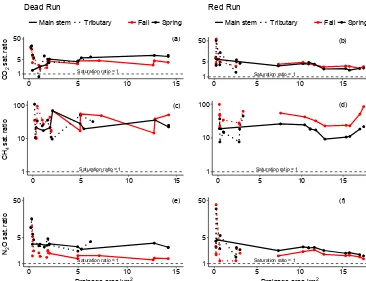
Spatial variability in GHG saturation was examined in or-der to evaluate whether concentrations measured in tribu-taries were consistent between headwaters and the larger third-order watersheds of Red Run and Dead Run respec-tively (Fig. 5). Multiple linear regressions yielded a set of distinct controlling factors on saturation of each gas. The op-timal models for CO2and N2O were similar and included the

log of drainage area, TDN concentration, log of discharge, and TDN×discharge interaction term. The CO2model also

included the DOC : TDN molar ratio. The optimal model for CH4saturation was slightly different and included the log of

drainage area, season (spring vs. fall), DOC concentration, and DOC : TDN molar ratio (Table 6). TDN concentration was not included in the optimal model for CH4. Watershed

location (tributary vs. main stem) was not included in the fi-nal model for any of the three gases.

2.7 Greenhouse gas emissions

GHG emission rates were sensitive to differences in mod-eledk600. Despite having medium-to-low gas saturation

ra-tios compared with other sites, DRKV had the highest GHG emission rates on all dates. This is due in part to having the highest slope (0.10 m m−1) and thus the highest mod-eled k600 (m d−1). Our 37 estimates of k600 ranged from

(a)

Saturation ratio = 1 1

5 50

0 5 10 15

C

O2

s

at

. r

at

io

Main stem Tributary Fall Spring

Dead Run

(c)

Saturation ratio = 1 1

10 100

0 5 10 15

C

H4

s

at

. ra

tio

(e)

Saturation ratio = 1 1

5 50

0 5 10 15

Drainage area km2

N2

O

s

at

. r

at

io

(b)

Saturation ratio = 1 1

5 50

0 5 10 15

Main stem Tributary Fall Spring Red Run

(d)

Saturation ratio = 1 1

10 100

0 5 10 15

(f)

Saturation ratio = 1 1

5 50

0 5 10 15

Drainage area km2

Figure 5.Longitudinal variability in CO2(a–b), CH4(c–d), and N2O(e–f)saturation ratios from spring and fall synoptic surveys of Dead Run and Red Run. Dotted lines denote tributaries to each watershed, while straight lines denote the main stem sites.

5.39±0.73 to 28.0±7.0 m d−1. The median value for all k600 estimates was 13.24 m d−1. This range of values and

site-averaged values extends beyond that measured by Pen-nino et al. (2014) of 0.5 to 9.0 m d−1. The discrepancy be-tween Pennino et al.’s (2014) k600 measurements is driven

by differences in channel gradient. Gradients in the present study ranged from 0.01 to 0.1, while Pennino’s ranged from 0.001 to 0.016 m d−1. Channel gradient (S) is also the param-eter with the greatest uncertainty, thus warranting cautious interpretation of our gas emission estimates.

Site-average CO2 emissions ranged from

6.4±2.3 g C m−2d−1 at DRAL (±standard error) to 134±30.2 at DRKV. Mean emission rates for DRGG and RRRB were 11.5±6.1 and 10.3±1.7 respectively. Site-average CH4emissions ranged from 2.6±1.1 at DRAL

to 102.5±75.6 mg C m−2d−1 at DRKV. N2O emissions

ranged from 5.1±0.8 at RRRB to 149±33.9 mg N m−2d−1 at DRKV. The full range of values and standard errors for fluxes are listed in Table 5.

3 Discussion 3.1 Overview

This study showed strong relationships between urban wa-ter quality and GHG saturation across streams draining

dif-ferent forms of urban infrastructure. N2O and CO2

satura-tion was correlated with nitrogen concentrasatura-tions but did not differ between infrastructure typologies. DOC : NO−₃ did dif-fer among the four infrastructure categories, however (Ta-ble 2). While infrastructure categories did not show a signif-icant predictor of GHG saturation in streams, the gradients in DOC : NO−₃ found across all categories were strongly cor-related with GHG saturation. Stoichiometric variation may thus serve as a predictor of GHG saturation downstream where land cover and infrastructure does not. While direct GHG loading to streams from leaky sanitary and/or stormwa-ter infrastructure may play a role, the strongest predictors of GHGs in this study were continuous/environmental vari-ables (i.e., TDN and DOC concentrations, DO, temperature), rather than categorical (infrastructure category). Relation-ships between anaerobic xsCO2-AOU and N2O saturation

further suggest that anaerobic metabolism contributes to N2O

production along hydrologic flow paths (Fig. 4). 3.2 C : N stoichiometry as an indicator of microbial

metabolism

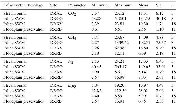
Table 5.Summary of gas flux estimations for the four sites with continuous flow data. Average, standard error (SE), and number of measure-ments (n) are listed for CO2(g C m−2d−1), CH4(mg C m−2d−), N2O (mg N m−2d−), and predictedk600(m d−1).

Infrastructure typology Site Parameter Minimum Maximum Mean SE n

Stream burial DRAL CO2 2.37 23.12 11.51 6.12 5

Inline SWM DRGG 53.28 548.01 134.55 30.18 3

Inline SWM DRKV 3.39 23.81 10.30 1.74 18

Floodplain preservation RRRB 0.61 5.51 2.55 1.10 11

Stream burial DRAL CH4 7.71 23.67 14.09 4.88 5

Inline SWM DRGG 2.27 1339.62 102.51 75.57 3

Inline SWM DRKV 3.26 62.98 16.80 5.29 18

Floodplain preservation RRRB 2.19 12.11 6.69 2.19 11

Stream burial DRAL N2 2.13 24.21 12.33 6.43 5

Inline SWM DRGG 60.45 565.17 149.63 33.91 3

Inline SWM DRKV 1.90 8.61 5.14 0.79 18

Floodplain preservation RRRB 2.57 16.98 7.03 2.63 11

Stream burial DRAL k600 3.84 19.20 10.97 4.47 5

Inline SWM DRGG 12.82 122.59 28.02 7.06 3

Inline SWM DRKV 2.40 8.89 5.39 0.73 18

Floodplain preservation RRRB 2.57 13.91 6.45 2.33 11

Table 6. Covariates and model fit parameters for linear models describing drivers of gas saturation ratios (CO₂, CH₄, and N₂O) from longitudinal surveys of Dead Run and Red Run. X’s denote that a given parameter was used in the final model while dashes (–) denote that parameters were not used.

Covariates tested CO2sat. ratio CH4sat. ratio N2O sat. ratio

Log of drainage area (km2) X X X

Watershed (Dead Run vs. Red Run) – – –

Season – X X

DOC (mg L−1) – X –

DIC (mg L−1) – – –

TDN (mg L−1) X – X

Log of Q (m3s−1) X – X

Location (tributary vs. main stem) – – –

DOC : TDN molar ratio X X –

TDN x log of drainage area interaction X – X

DOC x log of drainage area interaction – – –

Model AIC 336.85 542.14 263.59

Overall modelr2 0.789 0.153 0.795

Overall modelpvalue < 0.008 0.0082 < 0.008

(Fig. 4c) suggest that organic carbon availability modulates inorganic nitrogen loading to streams. DOC availability has been shown to control NO−₃ concentrations across terrestrial and aquatic ecosystems through a variety of coupled mi-crobial processes (Hedin et al., 1998; Kaushal and Lewis, 2005; Taylor and Townsend, 2010). Additionally, the average DOC : NO−₃ ratio (i.e., the slope of this relationship) varied significantly across categories. Variation in this relationship is likely driven by a combination of differential N loading across categories as well as different capacities for microbial N uptake and removal.

case, the higher C : N may have been driven by lower N leak-age rates as well as improved ecological function of the pre-served floodplain wetlands to remove any N that does enter the groundwater from stormwater or sewage leaks.

Understanding the spatial variability in N2O

concentra-tions, as well as the processes responsible for N2O

produc-tion and NO−₃ removal in watersheds, is useful for inform-ing watershed management. The relationship between N2O

and CO2 can provide insight into production mechanisms

because nitrification consumes CO2while denitrification

si-multaneously produces N2O and CO2. We found a strong

positive relationship between N2O saturation and CO2

con-centrations, suggesting that denitrification was the primary source of N2O (Fig. 5c). By contrast, very low DOC : NO−₃

ratios (Fig. 2) in stream water with the highest N2O

sat-uration (Fig. 3a) suggest that nitrification was the domi-nant process at these sites. Taylor and Townsend (2010) suggest that the ideal DOC : NO−₃ stoichiometry for deni-trification is 1:1 and that persistent conditions below that are more ideal for nitrification. DOC : NO−₃ was consis-tently below 1 in streams in septic system infrastructure, suggesting that in-stream denitrification would be carbon limited. We measured DOC : NO−₃ consistently above 1 at sites in riparian/floodplain preservation typology, suggest-ing NO−₃ was limiting for in-stream denitrification in this infrastructure category. Conversely, the mean stoichiomet-ric ratio was consistently near 1 in sites with inline SWM wetlands and stream burial, suggesting that denitrification may be occurring within the stream channel at these sites. While DOC : NO−₃ stoichiometry in watersheds with septic systems appeared more favorable for nitrification, the posi-tivexsCO2-AOU vs. N2O relationships in these streams

sug-gest that these gases were produced anaerobically (by deni-trification). One possible explanation for this discrepancy is that the N2O and CO2observed in the stream were produced

under stoichiometric conditions more favorable for denitri-fication along groundwater flow paths prior to emerging in the stream channel. Denitrification occurring along ground-water flow paths may draw down the DOC concentration as it is converted to CO2; however, the initial N load in

sep-tic plumes may be too high to nosep-ticeably decline. Pabich et al. (2001) documented this phenomenon, in which DOC con-centrations in a septic plume were quite high (> 20 mg L−1) in the upper part of the plume and declined exponentially, resulting in a very low DOC : NO−₃ ratio at depth.

Overall, the relationships between CH4 and CO2 were

much weaker and more variable than the relationships be-tween CO2and N2O (Fig. 4). While CO2and CH4are

some-times correlated in wetlands and rivers with low oxygen (Richey et al., 1998), this was not the case for our study sites. Instead, CO2 and N2O were highly coupled,

suggest-ing prevalence of NO−₃ as a terminal electron acceptor over CO2.

3.3 Effects of infrastructure on N2O saturation and

emissions

The present study documents some of the highest N2O

con-centrations currently reported in the literature for streams and rivers, ranging from 0.009 to 0.55 µM, with a median value of 0.07 µM and mean of 0.11 µM N2O-N. This range of

con-centration is greater than that reported for headwater agricul-tural and mixed land use streams in the Midwestern United States (0.03–0.07 µM, Werner et al., 2012; 0.03 to 0.15 µM, Beaulieu et al., 2008). A similar range of dissolved N2O

concentrations was reported for macrophyte-rich agricultur-ally influenced streams in New Zealand (0.06 to 0.60 µM, Wilcock and Sorrell, 2008). The only report of higher dis-solved N2O concentrations in streams is from a subtropical

stream receiving irrigation runoff, livestock waste, and urban sewage (saturation ratio maximum of 60 compared with 47 in this study; Harrison et al., 2005).

Average daily N2O emissions were high, ranging from

5.1 to 149.6 mg N2O-N m2d−1. Our value rates fall on

the high end compared with numerous studies of N2O

emission from urban and agriculturally influenced wa-terways, including agricultural drains in Japan (maxi-mum=179 mg N m2d−1; Hasegawa et al., 2000) or the Humber Estuary, UK (maximum=121 mg N m2d−1; Barnes and Owens, 1998). When the highest site (DRKV) is removed, these average daily fluxes remain high (range from 5.1 to 12.3 mg N m2d−1) compared with estimates reported for nitrogen-enriched agricultural and mixed land use streams in the Midwestern U.S. from Beaulieu et al. (2008) (mean=0.84 and maximum=6.4 mg N2

O-N m2d−1). Laursen and Seitzinger (2004) reported higher maximum rates (20 mg N m2d−1)to our overall median N2O

emission rates (13.8 mg N m2d−1)and the maximum daily rates measured in tropical agricultural streams in Mexico (mean=1.2 maximum=58.8 mg N2O-N m2d−1; Harrison

and Matson, 2003). While our measured N2O saturation

ra-tios were highly correlated solute concentrations and redox conditions (Table 4), emission rates were sensitive to the gas transfer velocity (k600), which varied by 2 orders of

magni-tude in our study (Table 6), and fell within the range of values estimated by Raymond et al. (2012).

Correlations between TDN and N2O concentrations in this

study highlight the role of urban N loading on GHG pro-duction along urban flow paths, which include groundwater, within pipes, and along the stream networks (Tables 3 and 4). While urban streams receive a mixture of different N sources including fertilizer, wastewater, and atmospheric deposition (e.g., Kaushal et al., 2011; Pennino et al., 2016), the location of aging gravity sewers adjacent to stream channels is likely to influence the relative importance of sewage on N and N2O

loading to streamwater. While this source of N2O emission is

(Gard-ner et al., 2016). N2O emissions from uncollected human

waste (i.e., leaky sanitary sewer lines, septic system efflu-ent, dug pits) are largely unmeasured globally (Strokal and Kroeze, 2014; UNEP, 2013) and warrant further study in the context of watershed management as well as local GHG ac-counting. Direct emissions from wastewater treatment plants are well documented (Foley et al., 2010; Townsend-Small et al., 2011; Strokal and Kroeze, 2014; UNEP, 2013); however, the upstream losses of N2O from delivery pipes into streams

and rivers are not well documented (Short et al., 2014). Short et al. (2014) measured N2O concentrations in WWTP

in-fluent in Australia and determined that sanitary sewers are consistently supersaturated with N2O, with concentrations

in excess of equilibrium by as much as 3.5 µM. Average daily sewer pipexsN2O concentrations were 0.55 µM, which

is nearly identical to the maximumxsN2O measured in the

present study (0.54 µM). While wastewater only contributes a portion of excess N in urban streams, further accounting for this source is necessary to improve municipal N2O budgets.

Synoptic surveys of N2O saturation in Red Run and Dead

Run in this study provide evidence that the entire network is a net source of N2O (Fig. 5). N2O saturation shows a

signif-icant decline with increasing drainage area (Table 6, Fig. 5), suggesting that emissions outpace new sources to the water column. Variability in gas concentration headwater sites and along the third-order stream networks is largely explained by a combination of discharge and/or drainage area as well as N concentrations and C : N stoichiometry in streamwater. 3.4 Effects of infrastructure on CH4saturation and

emissions

Methane was consistently supersaturated across all streams in this study and varied significantly across headwater infras-tructure categories. The highest CH4saturation ratios were

measured in sites with riparian reconnection (RRRM and RRRB) followed by streams draining inline SWM wetlands (DRKV and DRGG; Fig. 3 as with CO2). CH4saturation was

negatively correlated with DO; however, CH4was positively

correlated with DOC : NO−₃. CO2and N2O, by contrast, were

more strongly and positively correlated with TDN (Table 4). These patterns suggest that, along with redox conditions, car-bon availability may modulate CH4production as well.

CH4 concentrations in our study ranged from 0.06 to

6.08 µmol L−1, which is equivalent to the mean ±standard deviation of concentrations reported by a meta-analysis by Stanley et al. (2016). The saturation ratio (3.0 to 2157) fell within the lower range of previously measured values in agricultural streams in Canada (saturation ratio of 500 to 5000; Baulch et al., 2011a). Mean daily CH4 emissions

estimates in this study ranged from 2.6 to 103.5 mg CH4

-C m2d−1 and are comparable to measurements in agri-cultural streams of New Zealand (Wilcock and Sorrel, 2008; 17–56 mg CH4-C m2d−1)and southern Canada (20–

172 mg C m2d−1, Baulch et al., 2011); however, these

stud-ies also measured ebullitive (i.e., bubble) fluxes, whereas the present study only examined diffusive emissions. Stanley et al. (2016) reported the average of all current CH4

emis-sion rates to be 98.7 mg CH4-C m2d−1, with a minimum of −125.3 and a maximum of 5194 overall. While the CH4

emission estimates in the present study have a large margin of uncertainty due to the nature of estimating gas flux param-eters as well as the lack of ebullitive flux measurements, our sites were consistently sources to the atmosphere out the year at both headwater sites (Fig. 3) and through-out third-order drainage networks (Fig. 5b). Differences in CH4 abundance across infrastructure categories, as well as

the negative relationship between CH4saturation and TDN,

suggest that CH4may increase if TDN declines with the

ad-dition of stormwater wetlands and floodplain reconnection in urban areas.

4 Conclusions

Urban watersheds are highly altered systems, with heteroge-neous forms of infrastructure and water quality impairment. The present study demonstrates that N2O and CH4saturation

and emissions from urbanized headwaters are on the high end of estimates currently reported in the literature. Variations in urban infrastructure (i.e., SWM wetlands, riparian connectiv-ity, septic systems) influenced the C : N stoichiometry and re-dox state of urban streams. These in-stream variables, along with potential direct sources from leaky sanitary sewer lines, may contribute to increased GHG production and/or delivery to streams. Our results suggest that N from septic plumes and sanitary sewer lines is the principal source of N2O saturation

in our study sites. Dissolved inorganic N is highly correlated with N2O in our study sites, and the highest values are only

present in watersheds with aging sanitary sewer infrastruc-ture or septic systems. Our observations of N2O saturation

and emissions from urban and suburban headwater streams are comparable with streams and ditches in intensive agri-cultural watersheds (Harrison and Matson, 2003; Outram and Hiscock, 2012). These results suggest that streams draining medium-to-low-density suburban or exurban land cover are comparable to those in intensively managed agricultural ar-eas in terms of N2O emissions.

Code availability. The authors are happy to share any and all codes used to produce this paper. Please contact the corresponding author with inquiries about the codes used.

The Supplement related to this article is available online at https://doi.org/10.5194/bg-14-2831-2017-supplement.

Author contributions. R. Smith, S. Kaushal, C. Welty, and M. Pen-nino selected sampling sites based on infrastructure typology. R. Smith, S. Kaushal, and J. Beaulieu designed the gas and solute sampling design. R. Smith and J. Beaulieu analyzed samples for solute and gas concentrations respectively. C. Welty collected con-tinuous flow data from headwater gaging stations. J. Beaulieu pro-vided key insights into the interpretation of gas concentrations and statistical analyses and gas flux estimations. M. Pennino provided data used for estimatingK20. S. Kaushal and C. Welty provided funding for the project. All coauthors provided feedback on multi-ple versions of the manuscript.

Competing interests. The authors declare that they have no conflict of interest.

Acknowledgements. The authors gratefully acknowledge fund-ing from the National Science Foundation Water Sustainability and Climate program (NSF grants 1058038 and CBET-1058502) as well as the scientific infrastructure provided by the Baltimore Ecosystem Study LTER (www.beslter.org; NSF grant DEB-1027188). Field data collection was also partially supported by NOAA grant NA10OAR431220 to the Center for Urban Environmental Research and Education (http://cuere.umbc.edu) and the Water Resources mission area of the US Geological Survey (http://water.usgs.gov). Daniel Jones provided advice on spatial analyses, and numerous individuals including Tamara New-comer, Tom Doody, Evan McMullen, John Urban, Shahan Haq, Julia Gorman, Julia Miller, John Kemper, Erin Stapleton, and Joshua Cole provided field assistance and/or feedback on drafts of this manuscript. The views expressed in this article are those of the authors and do not necessarily reflect the views or policies of the US Environmental Protection Agency.

Edited by: T. J. Battin

Reviewed by: two anonymous referees

References

Aitkenhead-Peterson, J. A. and McDowell, W. H.: Soil C : N ratio as a predictor of annual riverine DOC flux at lo-cal and global slo-cales, Global Biogeochem. Cy., 14, 127, https://doi.org/10.1029/1999GB900083, 2000.

Alshboul, Z., Encinas-Fernandez, J., Hofmann, H., and Lorke, A.: Export of dissolved methane and carbon dioxide with effluents from municipal wastewater treatment plants, Envir. Sci. Tech. Lib., 50, 5555–5563, 2016.

Baltimore County Department of Planning: Master Plan 2010, available at: http://resources.baltimorecountymd.gov/ Documents/Planning/masterplan/masterplan2010.pdf (last access: 29 December 2015), 2010.

Baltimore County Government: GIS Data Download, available at: http://www.baltimorecountymd.gov/Agencies/infotech/GIS/ datadownload.html (last access: 9 May 2017), 2002.

Barnes, J. and Owens, N. J. P.: Denitrification and nitrous oxide concentrations in the Humber Estuary, UK, and adjacent coastal zones, Mar. Pollut. Bull., 37, 247–260, 1998.

Battin, T. J., Kaplan, L. A., Findlay, S. E. G., Hopkinson, C., Marti, E., Packman, A. I., Newbold, J. D., and Sabater, F.: Biophysi-cal controls on organic carbon fluxes in fluvial networks, Nat. Geosci., 1, 95–100, https://doi.org/10.1038/ngeo101, 2008. Baulch, H. M., Dillon, P. J., Maranger, R., and Schiff, S. L.:

Dif-fusive and ebullitive transport of methane and nitrous oxide from streams: Are bubble-mediated fluxes important? J. Geo-phys. Res., 116, 1–15, https://doi.org/10.1029/2011JG001656, 2011.

Beaulieu, J. J., Arango, C. P., Hamilton, S. K., and Tank, J. L.: The production and emission of nitrous oxide from headwater streams in the Midwestern United States, Glob. Change Biol., 14, 878–894, https://doi.org/10.1111/j.1365-2486.2007.01485.x, 2008.

Beaulieu, J. J., Arango, C. P., and Tank, J. L.: The ef-fects of season and agriculture on nitrous oxide produc-tion in headwater streams, J. Environ. Qual., 38, 637–646, https://doi.org/10.2134/jeq2008.0003, 2009.

Beaulieu, J. J., Shuster, W. D., and Rebholz, J. A.: Nitrous oxide emissions from a large, impounded river: the Ohio River, Envi-ron. Sci. Technol., 44, 7527–7533, 2010.

Beaulieu, J. J., Tank, J. L., Hamilton, S. K, Wollheim, W. M., Hall Jr., R. O., Mulholland, P. J., Peterson, B. J., Ashkenas, L. R., Cooper, L. W., Dahm, C. N., Dodds, W. K., Grimm, N. B., Johnson, S. L., McDowell, W. H., Poole, G. C., Valette, H. M., Arango, C. P., Bernot, M. J., Burgin, A. J., Crenshaw, C. L., Hel-ton, A. M., Johnson, L. T., O’Brien, J. M., Potter, J. D., Sheibley, R. W., Sobota, D. J., and Thomas, S. M.: Nitrous oxide emission from denitrification in stream and river networks, P. Natl. Acad. Sci., 108, 214–219, https://doi.org/10.1073/pnas.1011464108, 2011.

Beaulieu, J. J., Mayer, P. M., Kaushal, S. S., Pennino, M. J., Arango, C. P., Balz, D. A., Canfield, T. J., Elonen, C. M., Fritz, K. M., Hill, B. H., Ryu, H., and Santo Domingo, J.W.: Ef-fects of urban stream burial on organic matter dynamics and reach scale nitrate retention, Biogeochemistry, 121, 107–126, https://doi.org/10.1007/s10533-014-9971-4, 2014.

Beaulieu, J. J., Golden, H. E., Knightes, C. D., Mayer, P. M., Kaushal, S. S., Pennino, M. J., Arango, C. P., Balz, D. A., Elo-nen, C. M., Fritz, K. M., and Hill, B.: Urban Stream Burial In-creases Watershed-Scale Nitrate Export, Plos One, 10, e0132256, https://doi.org/10.1371/journal.pone.0132256, 2015.