A general Cluster data and global MHD simulation comparison

www.ann-geophys.net/26/3411/2008/ © European Geosciences Union 2008

Annales

Geophysicae

A general Cluster data and global MHD simulation comparison

P. Daum1, M. H. Denton1, J. A. Wild1, M. G. G. T. Taylor2, J. ˇSafr´ankov´a3, and M. Hayosh3

1_{Department of Communication Systems, Lancaster University, LA1 4WA Lancaster, UK}

2_{Science Operations Department, European Space Agency, 2201AZ Noordwijk ZH, The Netherlands} 3_{Faculty of Mathematics and Physics, Charles University, Prague, Czech Republic}

Received: 15 May 2008 – Revised: 11 August 2008 – Accepted: 27 August 2008 – Published: 4 November 2008

Abstract. Among the many challenges facing the space

weather modelling community today, is the need for val-idation and verification methods of the numerical models available describing the complex nonlinear Sun-Earth sys-tem. Magnetohydrodynamic (MHD) models represent the latest numerical models of this environment and have the unique ability to span the enormous distances present in the magnetosphere, from several hundred kilometres to several thousand kilometres above the Earth’s surface. This makes it especially difficult to develop verification and validation methods which posses the same range spans as the models. In this paper we present a first general large-scale compari-son between four years (2001–2004) worth of in situ Cluster plasma observations and the corresponding simulated pre-dictions from the coupled Block-Adaptive-Tree-Solarwind-Roe-Upwind-Scheme (BATS-R-US) MHD code. The com-parison between the in situ measurements and the model predictions reveals that by systematically constraining the MHD model inflow boundary conditions a good correlation between the in situ observations and the modeled data can be found. These results have an implication for modelling studies addressing also smaller scale features of the magne-tosphere. The global MHD simulation can therefore be used to place localised satellite and/or ground-based observations into a global context and fill the gaps left by measurements.

Keywords. Magnetospheric physics (Magnetopause, cusp,

and boundary layers; Solar wind-magnetosphere interac-tions) – Space plasma physics (Numerical simulation stud-ies)

Correspondence to: P. Daum

([email protected])

1 Introduction

The Earth’s magnetosphere is a highly complex nonlinear system mainly influenced by the interaction of the solar wind with the terrestrial magnetic field. The processes by which energy, mass, and momentum are transferred between these two domains is a primary focus of space physics research to-day. The dynamic processes controlling this highly disturbed near- to far-Earth plasma domain can reach from several kilo-metres to several thousand kilokilo-metres above the Earth’s sur-face. Modern satellite and ground-based measurements of this environment can only describe the processes and phe-nomena over limited spatial regions. They can be used as indicators for large-scale processes but in order to describe the physical processes on a global scale they often refer to three-dimensional numerical based models. By exploiting the full three-dimensional predictions of these models it is then possible to establish causal relationships between the localised observations and the global dynamics (Berchem, 2000). Here MHD codes represent the state-of-the-art com-putational models which are widely applicable and practical to execute in order to simulate the complex processes which are present in the geospace environment.

2008; Fedder et al., 1995, 1998, 2002; Gombosi et al., 2000; Hayosh et al., 2006; Palmroth et al., 2006; Pulkkinen et al., 1998; Raeder et al., 1997; Raeder, 2006; Siscoe et al., 2007; T´oth et al., 2007; Zhang et al., 2006). For these types of studies it is essential that the MHD simulations are precisely calibrated and constrained as outlined by Walker and Ashour-Abdalla (1995) and Berchem (2000) before they can be used to fill the gaps left by measurements and link the various lo-calised ground- and/or space-based observations. Validation and verification of the models therefore becomes indispens-able since only reliindispens-able model predictions can provide these links.

Whereas verification and validation methods in the com-puter science community are widely standardised (IEEE Standard 1012-1986/1998/2004) and well documented (e.g. Schlesinger, 1979; Adrion et al., 1982; Balci, 1997; Lipaev, 2003; Dasso and Funes, 2006) the same standards and tech-niques cannot be used for models of natural systems as out-lined by Oreskes et al. (1994). This is because natural sys-tems are never closed and because model results are always non-unique. Models can therefore only be verified and vali-dated to a certain degree by demonstrating an agreement be-tween observations and predictions and all confirmation is therefore inherently partial.

In addition to the lack of standardised verification and val-idation techniques, most modern MHD models are executed in “frameworks” and combine different numerical models in order to achieve the vast spatial coverage they offer. Each of these models can be seen as a module representing one spe-cific domain of the Sun-Earth system which are then coupled by control modules via standardised interfaces to achieve a global representation of the geospace environment. Simi-lar features in the observations of each individual domain within each module of the model provides a necessary but not sufficient condition for the “grand” MHD model (all ules coupled together) “validation”. Since the coupled mod-ules themselves represent a complete new model of a natural system, the coupled model itself needs to be validated by demonstrating an agreement between observations and pre-dictions. Based on the techniques for the verification and validation of large model systems described in Balci (1997) and Lipaev (2003) and in regards to the conclusions of the study by Oreskes et al. (1994) such combined models need two steps of “validation” before a general evaluation can be made; (1) each module on its own needs to be validated, (2) the combined and coupled modules need to be validated.

The second step consequently can only be used to evaluate the specific module configuration and has to be repeated ev-ery time the inner model configuration is changed. Whereas the first step of validation can be achieved via case and comparison studies utilizing localised ground- and/or space-based observations, the second relies on a large spatial cov-erage of the complete geospace environment to perform a reliable comparison between observations and predictions.

Recent case studies (Nozawa et al., 2001; Marsh and Roble, 2002; Mozzoni et al., 2007; Garner et al., 2004) have addressed the first step of validation of the different models describing the different sub-domains of the geospace envi-ronment; starting from the ionospheric electrodynamic (IE) models, through to the inner magnetosphere (IM) models, and further to the global magnetosphere (GM) models, but there exist only very limited studies addressing the second step of validation for the global coupled model (IE/IM/GM) runs. The existing studies rely mostly on limited spatial (few Earth radii) and temporal (few hours, several orbit progres-sions) comparisons between the model predictions and the observations and can therefore only be seen as a limited ap-proach for the second step of validation.

Our approach to this validation problem is presented in this study and based on the technique described in Den-ton and Taylor (2008) for the analysis of Cluster data sets. We utilize a large statistical sample (up to 825 000 data points; depending on the instrument) of magnetic field and plasma measurements from the Cluster spacecraft forma-tion collected in the years between 2001 and 2004, which are publicly available via the Cluster Active Archive (CAA: http://caa.estec.esa.int/caa/; Perry et al., 2006) and com-pare them to simulation runs of the Block-Adaptive-Tree-Solarwind-Roe-Upwind-Scheme (BATS-R-US) MHD code, coupled with the Rice Convection Model (RCM) and the Thermosphere Ionosphere Electrodynamic General Circula-tion Model (TIE-GCM). By using this large Cluster data set, we are able to achieve the vast spatial coverage needed for the second validation step. Thus, we attempt to validate the BATS-R-US/RCM/TIE-GCM coupled model to find con-straints and calibration factors to improve the model. By achieving a better accuracy of the model predictions, a bet-ter understanding of the physical processes present in the various domains can be achieved with implications of the model’s capabilities to enlarge the localised point-to-point measurements taken by ground- and/or space-based instru-ments.

2 Instrumentation/data analysis

The quartet of ESA Cluster spacecraft (Escoubet et al., 2001) were launched in July/August 2000 into a highly elliptical orbit(19.6 (apogee)/4.0 (perigee)RE). The orbital plane is fixed in the inertial frame of the Earth, therefore the apogee processes through 24 h of Local Time (LT) with a 12 month periodicity.

!20 !15 !10 !5 0 5 10 15 20 !20

!15 !10 !5 0 5 10 15 20

x_GSM [R_E] zGSM

[R

E

]

B z =!0.29nT nP = 6.03 #/cm3 v_sw=!477 km/s p = 2.3 nPa

ACE 235 R

E magnetopause

bowshock year: 2001!2004 days: 001!365

|B| = 0.07 nT

!20 !15 !10 !5 0 5 10 15 20 !20

!15 !10 !5 0 5 10 15 20

y_GSM [R_E] xGSM

[R

E

]

ACE235 R

E

data range magneto! pause bowshock

!20 !15 !10 !5 0 5 10 15 20 !20

!15 !10 !5 0 5 10 15 20

y_GSM [R_E]

zGSM

[R

E

]

data range

magneto!

pause

bowshock

Fig. 1. Plots showing thex–z,x–y, andy–zGSM projections of the Cluster 1 (Rumba) orbit for the time period from 1 January 2001 to 31 December 2004 in 100 min resolution for every 10th full orbit. Overlaid are the modeled magnetopause shape (Shue et al., 1997) indicated by the solid grey lines and the modeled bowshock shape (Bennett et al., 1997) indicated by the dashed grey lines. The models are parameterised by the solar wind and IMF conditions as shown in the upper right hand corner of the left-hand panel. In thex–yGSM projection (centre panel) the dayside magnetosphere area which is swept over by the orbit in the first 120 days of each year is highlighted by an underlying grey area. In thex–yand they–zGSM projections the Cluster orbits falling into a range of±5REofy=0REare highlighted in yellow and represent the data range for the performed comparisons.

(Bennett et al., 1997) indicated by the dashed grey lines. The models are parameterised by the averaged solar wind and in-terplanetary magnetic field (IMF) conditions for the time of interest as shown in the upper right hand corner of thex–z

GSM projection (left-hand panel). The solar wind parame-ters were obtained from the Solar Wind Electron, Proton, and Alpha Monitor (SWEPAM; McComas et al., 1998), and the IMF conditions were obtained from the Magnetic Field Ex-periment (MAG; Smith et al., 1998) onboard the Advanced Composition Explorer (ACE) satellite (Stone et al., 1998). The utilised data were accessed via the ACE Science Center (ASC: http://www.srl.caltech.edu/ACE/ASC/; Garrard et al., 1998). As shown in Fig. 1 the Cluster orbit offers a great spa-tial coverage of the near-Earth plasma environment stretch-ing from ±19.4RE in x- and y-GSM direction and from ±12.5REinz-GSM direction. The measurements taken dur-ing the four years of interest offer an extensive data set for the validation of the coupled MHD model.

For the comparison between the Cluster measurements and the MHD model predictions we use the plasma parti-cle observations from the Cluster Ion Spectrometry (CIS) in-strument (R`eme et al., 1997, 2001) and the magnetic field measurements taken by the Cluster fluxgate magnetometer (FGM) instrument (Balogh et al., 1997, 2001). The measure-ments of the ion distribution function in the energy ranges from∼0–40 keV obtained from the Composition and Distri-bution Function (CODIF) sensor of the CIS instrument that allows calculations of the moments of the distribution and thus provides averaged values for temperature, density, and velocity. These data combined with the magnetic field ponents obtained from the FGM instrument allow us a

com-parison with the prime MHD model output parameters (see Sect. 3, Fig. 2).

To allow an efficient analysis of this extensive in situ data set, we apply the technique first described in Denton and Tay-lor (2008). The derived and observed individual parameters (density, pressure, temperature, magnetic field strength, and velocity components) are first interpolated to a time resolu-tion of one minute. Following this temporal interpolaresolu-tion the parameters are binned according to the location of the Clus-ter spacecraft onto an equidistal cartesian grid with a size of 1×1RE and averaged values within each bin are calcu-lated. By combining several of these data files it is then possible to produce quasi two-dimensional representations of the geospace environment at any given location. To enhance the data range of these “data-planes”, measurements taken in an orbital position within a perpendicular distance of±5RE from the required plane are used as complement. Figure 1 highlights this technique in the case for anx–zGSM plane at

y=0RE, here all measurements taken in an orbital position which falls into a range of±5RE(highlighted in yellow) are used to make up the data range of thex–zGSM data-plane. Following these criteria averaged data-planes of all before mentioned prime plasma parameters can be created.

!"#$%"&'%!()*#+,-).)

/!'0$%*+1.12+3

45567&'8956:;<=>676 /4'0.?'3

4;5;<=>676 )@6A:7;BC58DEA<

/4)0*4)1!?'3

FE6

@B

1%

@E9

56

B

?

G7

76

5:<

)

@6

A:

7E

A&

,

;:

65

:E8

@ !"#$%&!'%(#!)*+%,-./%&0*#+%#0"*) 1 =;E5:<&;H&E5:67<6A:E;5&;H&:>6&

!1"!+'&6IG8:;7E8@&=@856 1 D89J&HE6@B&<:7659:> 1 D89J&H@GK&:GL6&M;@GD6 1 8M67896B&B65<E:C& 1 8M67896B&=76<<G76

N6

5<

E:C

0&

,

76

<<

G7

6

)@6A:7EA ,;:65:E8@

(%!

%1

%2

%#%*

%+

%%%,

%!

%+

%1

%#%*

%)

%%3

%4

%5

%6%7

%5

%6%7

%8

%9

!

1

%:%2

%1

%:

3;9%%B65<E:C&/!3 3<9%%M6@J&A;D=J&/"#O"$O"%3

3=9%%=76<<G76&/&3 3>96@6AJ&AG7765:&A;D=J&/'#O&'$O&'%3

3?9%%D89J&HE6@B&A;D=J&/(#O&($O&(%3&&&&&&&&&3@9 -8@@&85B&,6B67<;5&A;5BJ&/!-O!,3&

Fig. 2. Coupling scheme of the GM (Block-Adaptive-Tree-Solarwind-Roe-Upwind-Scheme), the IM (Rice Convection Model), and the IE (Thermosphere Ionosphere Electrodynamic General Circulation Model) modules.

to identify and exclude times where extreme solar wind con-ditions (high solar wind speeds and high proton densities) were present. The data points therefore can vary according to time and selected orientation of the data-plane. For the here presented study we mainly usex–z(noon-midnight merid-ian plane) GSM andx–y(equatorial) GSM data-planes with data sets consisting of 80 000 to 825 000 points.

In addition to the physical limitations of the instruments also the fact that Cluster 1 (Rumba) does not operate an ac-tive spacecraft potential remediation mechanisms has to be accounted for. Depending upon ambient plasma conditions, this can affect how well the distributions (and hence the de-rived moments) represent the actual local plasma conditions. The effect is most obvious when the plasma contains a very hot (or very cold) component with energies beyond the range of the instrument. Hence, as noted by Denton and Taylor (2008), the resultant plasma densities shown are likely to un-derestimate the actual values. It should be noted here, that in the high flux regions (cusps, magnetosheath) the spacecraft potential is quite low (<10 V) and so does not affect the CIS instrument measurements as much as in the plasma sheet and in particular the lobe region. These issues should be borne in mind not only when interpreting the results presented below, but when utilising any thermal plasma measurement. How-ever, a comparison between densities measured on Cluster 1 (Rumba) and densities from other Cluster spacecraft where active spacecraft potential control is operating shows little quantitative difference. Therefore for the statistical purpose of this study the differences are negligible.

3 MHD model (coupled modules GM/IM/IE)

The corresponding MHD study uses simulation results from the coupled BATS-R-US MHD code (Powell et al., 1999), which was originally developed by the Computational MHD Group at the University of Michigan, now the Center for Space Environment Modeling (CSEM: http://csem.engin. umich.edu). The code used is version 7.73 which is part of the Space Weather Modeling Framework (SWMF: http://csem.engin.umich.edu/swmf/) described by T´oth et al. (2005) and Volberg et al. (2005). The BATS-R-US code solves three-dimensional MHD equations in a finite volume form using numerical methods related to Roe’s Approximate Riemann Solver (Roe, 1981). The code employs an adap-tive grid composed of rectangular blocks arranged in varying degrees of spatial refinement levels. A detailed description of the model and the numerical/parallel implementation can be found in Gombosi et al. (2003). The BATS-R-US MHD code represents the GM module of the here discussed cou-pled simulation.

The IM module is described by the RCM which represents the inner and middle magnetosphere with a coupling to the ionosphere (Toffoletto et al., 2003). The RCM represents the particles in terms of multiple fluids. Its equations and nu-merical methods have been especially designed for an accu-rate treatment of the inner magnetosphere, including the flow of electric currents along magnetic field lines to and from the conducting ionosphere. The RCM computes these cur-rents and the associated electric fields self-consistently. It assumes perfectly conducting field lines and employs a pre-computed time-dependent magnetic field with associated in-duction electric fields. The Vasyliunas equation (Vasyliunas, 1970) is used to compute the magnetic-field-aligned currents (Birkeland currents), and Ohm’s law is used to compute the self-consistent ionospheric potential distribution. A detailed description of the BATS-R-US/RCM coupling can be found in De Zeeuw et al. (2004). The IE module is described by the TIE-GCM code (Ridley and Liemohn, 2002; Ridley et al., 2004). It is a two-dimensional electrostatic potential solver that obtains the field-aligned currents from the global magne-tosphere (GM) module included in the SWMF and employs a statistical auroral ionosphere conductance model driven by the solar irradiation index (F10.7) and by the field-aligned current patterns.

The three modules (GM/IM/IE) are then coupled un-der the SWMF to form a consistent representation of the geospace environment. The coupling is achieved with near-continuously two-way flow information between the differ-ent modules via standardised interfaces. A schematic of the coupling is presented in Fig. 2. We shall only briefly out-line the fundamental coupling aspects and refer to De Zeeuw et al. (2004) and T´oth et al. (2004, 2005) for a detailed de-scription.

0 10

Dens. [#/cm

!

3]

Jan!Apr (1) Jan!Apr (2) Jan!Apr (3) Jan!Apr (4)

a)

0 20

Temp. [K]

104 b)

!700 !600 !500 !400

vx GSM

[km/s]

c)

!20 0 20

vy GSM

[km/s]

d)

!20 0 20

vz GSM

[km/s]

e)

!10 0 10

Bx GSM

[nT]

f)

!10 0 10

By GSM

[nT]

g)

!5 0 5

Bz GSM

[nT]

h)

2001 2002 2003 2004 2005

!100 0 100

clock angle [°]

Year i)

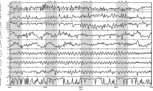
Fig. 3. Solar wind and IMF conditions (model upstream input boundary conditions) obtained from the ACE satellite between 2001–2004 in six day averages. The first panel (a) represents the solar wind density, the light grey trace in this panel represents the 50% decrease of the solar wind density used in the model runs. The second panel (b) represents the temperature. The following panels represent from (c)–(e) the GSMvx,vy,vzcomponents of the solar wind, and (f)–(h) the GSMBx,By,Bzcomponents of the interplanetary magnetic field, (i) shows the IMF clock angle (defined as arctan By/Bz). The periods when the Cluster orbit swept over the dayside magnetosphere (first 120 days of each year; cf. Fig. 1 centre panel) are highlighted with underlying grey areas.

magnetosphere. Starting from these calculations closed field line positions are determined and their intersections with the equatorial plane are passed to the IM module along with the overall magnetic field strength, the magnetic flux tube vol-umes, and the corresponding pressure and density values. IM derives its plasma distribution outer boundary and supplies the time-evolving plasma density and pressure on its spheri-cal grid to adjust the GM values.

The IM and IE modules are only one-way coupled, the IE takes the field-aligned currents from the GM module, the electric potential of the IE calculations is then passed back via the IM to the inner GM boundary.

This GM/IM/IE coupling allows us to retrieve a wide range of output parameters from the different domains of in-terest. The model outputs (cf. Fig. 2) include the plasma pa-rameters (atomic mass unit densityn; kinetic pressurep; ve-locityvx,vy,vz), the magnetic field componentsBx,By,Bz, and the electric current componentsjx,jy,jz (prime model outputs) as well as ionospheric electrodynamic parameters (electric potential 8; Hall and Pedersen conductance6H,

6P) and the ionospheric electric current densityJ. We shall not further comment on the electrodynamic parameters since

a comparison of these data sets is not in the scope of this pa-per. It should be noted, that the IE module is only included in the coupled simulation for completeness to represent the most commonly used coupled simulation run especially for coordinated ground- and space-based studies. The IE mod-ule is not neglectable since a change in the configuration of the coupled modules would represent a complete new natural system which then again would need validation as outlined by Oreskes et al. (1994) and Lipaev (2003).

±21RE. Since the CCMC is running the SWMF version 2.1 and the Lancaster HPC is running version 2.3 with a different CPU layout an initial test of the simulation results was per-formed by comparing the two runs. This step serves as first verification level to rule out computational and numerical er-rors which could arise from the different CPU layouts and the different compiler infrastructures used. The runs showed equivalent results so that we are confident in using the simu-lation run results for the comparison with the averaged bulk plasma parameters obtained from the instruments onboard the Cluster spacecraft.

The global MHD simulation is driven by real upstream so-lar wind conditions (see Fig. 3) of the y–z GSM plane at

x=33RE, at the other boundaries the code assumes a zero gradient for the plasma variables since these boundaries are far enough from the Earth that they have no significant ef-fect on the dynamics due to the fact that they introduce a negligible effect in the resistive MHD equations describing the domain. Since a real time simulation run over the com-plete time span (2001–2004) was not operable (each time step in the simulation represents a full three-dimensional bounding box calculation with over 22.8 million data points), we have calculated six day averages from the hourly ACE Level 2 merged IMF, solar wind, and energetic particle data files. Figure 3 presents an overview of these six day aver-aged data sets from 2001 to 2004. The first panel shows the solar wind density (also the 50% decrease, light grey trace which was used in the simulation runs as constraining fac-tor) followed by the solar wind temperature, the velocity, and magnetic field strength components in a GSM reference frame. The last panel shows the IMF clock angle defined as arctan By/Bz. With these six day averaged solar wind and IMF conditions a quasi time-accurate simulation was per-formed and every cadence in the simulation therefore rep-resents a six day cadence in real-time. Subsequently with the 243 dependent IMF and solar wind condition also 243 model outputs with an average dipole tilt of 0◦ (corresponding to the four years observation time) were computed and used for the comparison.

For the times where the Cluster orbit swept over the day-side magnetosphere region, highlighted in Fig. 3 by the un-derlying grey areas, additional fixed input boundary model runs with an averaged dipole tilt of−11.68◦(calculated from the daily dipole tilts in the time from January to April of each year) were performed. These runs were then used for an ini-tial comparison of the magnetopause shape and location in the model and the data in order to give a first implication if the presented constraining factor (50% density decrease) is applicable. It has to be noted here, that the model runs with fixed input boundary conditions converge into a steady-state solution through unphysical intermediate solutions but since we only use these runs for a comparison of the directly driven part of the magnetosphere reasonable implications for the constraining factor can be drawn.

4 Comparison

The model and data comparison contains two steps. The first step develops and evaluates the constraining factor used for the model runs and the second then builds upon this factor to present a first general large-scale comparison of the Cluster observations and the coupled MHD model run predictions. 4.1 Initial comparison

As outlined in the studies by Daum and Wild (2006) and Hayosh et al. (2003, 2006) using the coupled BATS-R-US model (GM/IM/IE) in comparison with high-latitude Cluster and high-/low-latitude INTERBALL-1 observations respec-tively, the coupled model seems to overestimate the general magnetic field and plasma compression. Therefore the bow-shock and magnetopause boundary is pushed further towards the Earth as indicated by the in situ satellite observations. In order to compensate for this and to “calibrate” the model, a constraining factor for the upstream input boundary condi-tions is necessary. As shown in Fig. 2 the parameter which has a direct linear influence on the coupling between the GM and IM module is the solar wind proton density, this factor then also determines the location and shape of the bowshock and the magnetopause in the simulation. In respect to the results presented by Daum and Wild (2006); Hayosh et al. (2003, 2006); Koval et al. (2006) we have computed differ-ent simulation runs (not shown here) with varying densities (from 100% to 30% of the original value) and have compared the location of the magnetopause in these simulation runs with actual Cluster magnetopause crossings. Therefore we used the simulated data to estimate the times of the Cluster magnetopause crossings exploiting the spacecraft orbit path and the prime model output parameters. The crossing times were identified manually on the basis of several independent criteria of changing fields along the orbit path: (1) the mag-netic field variations in strength and direction, (2) sudden increases in the x-GSM velocity component, and (3) loca-tions/regions where the vector field of∇p−pdiffers from zero and exhibits a drastic magnitude change. The so de-duced times of crossing were then compared with the actual in situ field and plasma indications observed by the instru-ments. Here the simulation runs performed with density de-creases of∼50%±3% showed the best agreement between the predicted times and the actual times of the magnetopause crossings.

!20 !15 !10 !5 0 5 10 15 20 !20 !15 !10 !5 0 5 10 15 20

x_GSM [R_E] zGSM

[R

E

]

year: 2001

days: 001!120 |B| = 0.49_B nT z =!0.3 nT nP = 6.5 #/cm3 vsw=!449 km/s p = 2.2 nPa T = 93444 K

ACE

235 RE magnetopause

bowshock

CPQSTER 1 orbit projection (1)

!20 !10 0 10 20 !20 !15 !10 !5 0 5 10 15 20

x_GSM [R_E] zGSM

[R

E

]

CLUSTER 1 data | 2001 | GRID 1.00 R_E

av. dipole tilt !11.68°

PRESSURE [nPa] 0 0.1 0.2 0.3 0.4 0.5 0.6 0.7 0.8

x_GSM [R_E] zGSM

[R

E

]

BATS!R!US / RCM | 2001 | GRID 0.50 R_E

av. dipole tilt !11.68°

!20 !10 0 10 20 !20 !15 !10 !5 0 5 10 15 20 PRESSURE [nPa] 0 0.1 0.2 0.3 0.4 0.5 0.6 0.7 0.8 !20 !15 !10 !5 0 5 10 15 20 !20 !15 !10 !5 0 5 10 15 20

x_GSM [R_E]

zGSM

[R

E

]

year: 2002

days: 001!120 |B| = 1.1 nT

B

z = 0.58 nT

nP = 7.3 #/cm3

vsw=!446 km/s

p = 2.4 nPa

T = 101318K

ACE 235 R

E magnetopause

bowshock

CQRSTER 1 orbit projection (2)

!20 !10 0 10 20 !20 !15 !10 !5 0 5 10 15 20

x_GSM [R_E] zGSM

[R

E

]

CLUSTER 1 data | 2002 | GRID 1.00 R_E

av. dipole tilt !11.68°

PRESSURE [nPa] 0 0.1 0.2 0.3 0.4 0.5 0.6 0.7 0.8

x_GSM [R_E] zGSM

[R

E

]

BATS!R!US / RCM | 2002 | GRID 0.50 R_E

av. dipole tilt !11.68°

!20 !10 0 10 20 !20 !15 !10 !5 0 5 10 15 20 PRESSURE [nPa] 0 0.1 0.2 0.3 0.4 0.5 0.6 0.7 0.8 !20 !15 !10 !5 0 5 10 15 20 !20 !15 !10 !5 0 5 10 15 20

x_GSM [R_E]

zGSM

[R

E

]

year: 2003

days: 001!120 |B| = 0.47_B nT

z =!0.22 nT

nP = 6 #/cm3

vsw=!515 km/s

p = 2.7 nPa

T = 140970K

ACE 235 R

E magnetopause

bowshock

CQRSTER 1 orbit projection (3)

!20 !10 0 10 20 !20 !15 !10 !5 0 5 10 15 20

xGSM [RE] zGSM

[R

E

]

CLUSTER 1 data | 2003 | GRID 1.00 R_E

av. dipole tilt !11.68°

PRESSURE [nPa] 0 0.1 0.2 0.3 0.4 0.5 0.6 0.7 0.8

xGSM [RE] zGSM

[R

E

]

BATS!R!US / RCM | 2003 | GRID 0.50 R_E

av. dipole tilt !11.68°

!20 !10 0 10 20 !20 !15 !10 !5 0 5 10 15 20 PRESSURE [nPa] 0 0.1 0.2 0.3 0.4 0.5 0.6 0.7 0.8 !20 !15 !10 !5 0 5 10 15 20 !20 !15 !10 !5 0 5 10 15 20

x_GSM [R_E]

zGSM

[R

E

]

year: 2004

days: 001!120 |B| = 0.22_B nT

z =!0.17 nT

n

P = 4.8 #/cm3

v

sw=!500 km/s

p = 2 nPa T = 135165K

ACE

235 R

E magnetopause

bowshock

CQRSTER 1 orbit projection (4)

!20 !10 0 10 20 !20 !15 !10 !5 0 5 10 15 20

xGSM [RE]

zGSM

[R

E

]

CLUSTER 1 data | 2004 | GRID 1.00 R_E

av. dipole tilt !11.68°

PRESSURE [nPa] 0 0.1 0.2 0.3 0.4 0.5 0.6 0.7 0.8

xGSM [RE] zGSM

[R

E

]

BATS!R!US / RCM | 2004 | GRID 0.50 R_E

av. dipole tilt !11.68°

!20 !10 0 10 20 !20 !15 !10 !5 0 5 10 15 20 PRESSURE [nPa] 0 0.1 0.2 0.3 0.4 0.5 0.6 0.7 0.8

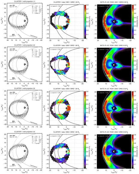
distributions. Overlaid are the magnetopause boundary af-ter Shue et al. (1997) and the bowshock shape afaf-ter Bennett et al. (1997) parameterised by the averaged IMF and solar wind conditions as shown in the upper right hand corner of each of the orbit projections. The averaged dipole tilt for the times of interest is indicated by the−11.68◦tilted day-/nightside representation of the Earth.

The observational results shown in the second column of Fig. 4 agree with similar studies previously published (Es-coubet et al., 1997; Lavraud et al., 2004; Denton and Tay-lor, 2008) and exhibit the classical distinguishable plasma re-gions. From left to right; the solar wind, then the compressed magnetosheath followed by the inner plasmasphere. Assum-ing that the Cluster data-planes are representative of the av-erage dayside magnetosphere state for the times of interest, we can now compare these data-planes with corresponding simulation runs. Therefore we have used the averaged so-lar wind and IMF conditions present at the four time spans (see (1), (2), (3) and (4) in Fig. 3) when Cluster was located in the dayside magnetosphere and have computed the cor-responding coupled MHD predictions. The model runs were performed with fixed input boundary condition (shown in the upper right hand corner of the orbit projections) but with a 50% decrease of the solar wind proton density and a fixed dipole tilt of−11.68◦was used. Figure 4 third column shows the colour-codedx–zGSM pressure distributions aty=0RE for the BATS-R-US/RCM/TIE-GCM coupled model runs. Also here the bowshock shape (Bennett et al., 1997) and the magnetopause boundary (Shue et al., 1997) are overlaid.

Comparing the in situ pressure distributions with the mod-eled ones, it can be seen that both modelled and measured pressures exhibit three distinct plasma regimes and their as-sociated boundaries after Bennett et al. (1997) and Shue et al. (1997). Here it should be noted, that the bowshock model seems to perform slightly better than the magne-topause model especially in the tailward flank regions. But as shown in ˇSafr´ankov´a et al. (2002) these variations are com-mon for second order surface fits as used in the Shue et al. (1997) model and spreads of 2RE to 3REinside or outside the model surface are expected. Therefore the slight vari-ances between the here employed MHD model and the mag-netopause representation are expected. Both boundaries can therefore be used as reference for the following comparison and give a first indication of the applicability of the constraint used.

Following on from this initial referential comparison it can be seen that from the solar wind to the compressed magne-tosheath region, the model as well as the data show a steep gradient in the pressure with similar values and distributions upstream and downstream of the bowshock. Inside the mag-netosheath region the pressure values raise up top0.8 nPa. Here the observations exhibit the highest values in the north-ern and southnorth-ern cusp regions (x∼7RE andz∼±7RE) and the model data exhibit the highest values at the subsolar nose region (x∼10RE andz∼3RE) which then extend into the

cusps. At a normal distance of 1RE to 3RE downstream of the magnetopause boundary the values drop again to lev-els of around 0.1–0.2 nPa. Here the two tail lobes above and beneath the neutral sheet become apparent. Continuing in-wards to the nightside of the Earth at lower L-shell positions, the values raise again to magnetosheath level. This steep gra-dient in the observations is not present in the model data and suggests that the model underestimates the nightside plasma injection in L-shell regions under 3RE.

As outlined in De Zeeuw et al. (2004); Danov and Koleva (2007); Garner et al. (2004); Lemon et al. (2004, 2005) this underestimation is common in the coupled IM module and is heavily dependent upon the initialisation time given for the model run, until its sets into a steady state for the ring current distribution and it is dependent on the grid resolution used. The grid resolution change between the GM and IM module can cause diffusion regions which then have an influence on the current distribution and subsequently the plasma pressure distribution especially in the near-Earth regions. In the case presented here it is most likely that the underestimation is the result of the fixed input boundary conditions since the model runs therefore do not include the temporal (120 days) and spatial (±5RE perpendicular to y=0RE) variations of the high-energetic plasma processes (unlike the observations).

Overall it can be said that the coupled MHD simulation re-produces reasonable well the actual statistical parameterisa-tion of the dayside magnetosphere given by the observaparameterisa-tions and clearly exhibits the three main plasma regions separated by the boundary representations of Bennett et al. (1997) and Shue et al. (1997). Whereas with the 50% decrease these boundaries are reproduced reasonably well the>60% den-sity runs (not shown here) put the location of the bowshock and the magnetosphere further towards the Earth due to their overestimation of the magnetic field and plasma compres-sion. We are therefore confident in using the 50% decrease of the solar wind proton density as a constraining factor to calibrate and adjust the MHD model runs.

4.2 General comparison

!20 !10 0 10 20 !20 !15 !10 !5 0 5 10 15 20

xGSM [RE] zGSM

[R

E

]

CLUSTER 1 data | 2001!2004 | GRID 1.00 R_E

av. dipole tilt 0°

(a) PRESSURE [nPa] 0 0.1 0.2 0.3 0.4 0.5 0.6 0.7 0.8

xGSM [RE] zGSM

[R

E

]

BATS!R!US / RCM | 2001!2004 | GRID 0.50 R_E

av. dipole tilt 0°

(b) !20 !10 0 10 20 !20 !15 !10 !5 0 5 10 15 20 PRESSURE [nPa] 0 0.1 0.2 0.3 0.4 0.5 0.6 0.7 0.8 !20 !10 0 10 20 !20 !15 !10 !5 0 5 10 15 20

x_GSM [R_E] zGSM

[R

E

]

a0. dipole tilt 0°

(c)

C;USTER 1 data / BATS!R!US | GRID 1.00 R_E

! PRESSURE [nPa] 0.00 0.05 0.10 0.15 0.20 0.25 0.30 0.35 0.40 !20 !10 0 10 20 !20 !15 !10 !5 0 5 10 15 20

y_GSM [R_E] xGSM

[R

E

]

CLUSTER 1 data | 2001!2004 | GRID 1.00 R E

av. dipole tilt 0°

(d) PRESSURE [nPa] 0 0.1 0.2 0.3 0.4 0.5 0.6 0.7 0.8

y_GSM [R_E]

xGSM

[R

E

]

BATS!R!US / RCM | 2001!2004 | GRID 0.50 R E

av. dipole tilt 0°

(e) !20 !10 0 10 20 !20 !15 !10 !5 0 5 10 15 20 PRESSURE [nPa] 0 0.1 0.2 0.3 0.4 0.5 0.6 0.7 0.8 !20 !10 0 10 20 !20 !15 !10 !5 0 5 10 15 20

y_GSM [R_E] xGSM

[R

E

]

av. dipole tilt 0°

(f)

CLUSTER 1 data / BATS!R!US | GRID 1.00 R E ! PRESSURE [nPa] 0.00 0.05 0.10 0.15 0.20 0.25 0.30 0.35 0.40

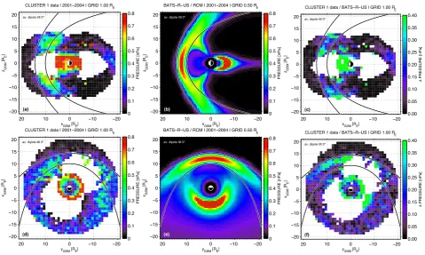
Fig. 5. Cluster 1 (Rumba) data and model comparison in thex–zandx–yGSM planes for the time from 2001 to 2004 with up to 825 000 data points; (a)/(d) plasma pressure measurements, (b)/(e) MHD model predictions, and (c)/(f) resultant deviation. Overlaid are the magnetopause boundary (Shue et al., 1997) and the bowshock shape (Bennett et al., 1997) parameterised by the IMF and solar wind conditions as previously shown in Fig. 1.

the empirical Tsyganenko (T’96) magnetic field model (Tsy-ganenko, 1995; Tsyganenko and Stern, 1996) predictions. Overlaid on all resultant maps are the magnetopause bound-ary (Shue et al., 1997) and the bowshock shape (Bennett et al., 1997) parameterised by the averaged IMF and solar wind conditions obtained from the six day averages as shown in Fig. 3.

4.2.1 Pressure comparison

The x–z GSM pressure maps of the observations and the model (see Fig. 5a–e) exhibit again the three clear distin-guishable plasma regions with similar values and distribu-tions. By using the complete Cluster data set, the night-side distribution is also shown and exhibits, in addition to the above described characteristics, a slight increase of pres-sure in the far tail region atx∼−15RE with values raising to about 0.3 nPa. This is reproduced by the model but with a much thinnerz-GSM spread, this is due to the fact that the model uses a fixed 0◦ dipole tilt whereas the observa-tions include the daily and annual variaobserva-tions. Figure 5c also shows that the Cluster data and the model predictions devi-ate the most on the dayside inner plasmasphere atx∼3RE, here a difference of upto 0.4 nPa can be observed. Elsewhere

the model predictions and the Cluster data are in reasonable agreement with a standard deviation of∼0.13 nPa.

In thex–y GSM pressure map of the observations (see Fig. 5d) the clearly distinguishable plasma regions men-tioned previously blend into each other and only two clear regions are apparent, the solar wind and the quasi com-bined magnetosheath and magnetosphere. It should be noted that the observations do not include values in the

5RE<x<10RE,−10RE<y<0RE region (also the inverse

is true for the nightside) due to the orbit path and therefore only limited comparisons can be made. The data do not show the three plasma regions and clearly defined boundaries pre-sented in the model predictions, with high plasma pressure values inside the magnetosheath and lower pressure values downstream of the dayside magnetopause. In the inner plas-masphere the model and the observations have a better agree-ment but the model exhibits smoother gradients, this is also reflected in the deviation plot see Fig. 5f.

year: 2001 day: 096

CRCM model of the ring current fluxes

y

GSM [RE] xGSM

[R

E

]

x104

B_z =!0.93 nT nP = 3.93 #/cm3 v_sw=!614 km/s p = 3.27 nPa

!10

!5 0

5 10

!10

!8

!6

!4

!2 0 2 4 6 8 10

PROTON FLUX [1/(cm

2 s sr keV)]

0 1 2 3 4 5

Fig. 6. Colour-coded proton flux in the equatorial plane derived from the one-way coupled RCM and Fok et al. (2001) model. Over-laid is the magnetopause boundary after Shue et al. (1997) parame-terised by the IMF and solar wind condition as shown in the lower right hand corner.

is consistent with the results presented by e.g. Antonova et al. (1999); De Michelis et al. (1999); Lui (2003). These near-Earth high plasma values encounters are not well reproduced by the model.

Comparing the simulation runs with the results presented in Lemon et al. (2004, 2005) a consistency can be found. The magnetic-field perturbations in the RCM model seems to prevent the injection of a significant ring current and sub-sequently prevent the occurrence of a high plasma pressure in the near-Earth region. In order to get a fully self-consistent representation of the near-Earth environment, the RCM has to be further coupled with a ring current model. At the cur-rent state the SWMF does include a coupling between the RCM and the Fok et al. (2001) ring current and radiation belt model. But, this so called Comprehensive Ring Cur-rent Model (CRCM) is strictly one-way coupled and does not interfere or alter the general GM/IM/IE MHD simula-tion. Therefore it can be used for case studies addressing this specific plasma domain but can not be included in the general validation of the coupled MHD model under investi-gation here. For completeness and since it does not interfere with the general simulation in the sense of changing the nat-ural system (Oreskes et al., 1994), in addition to the MHD model steps we have also computed the corresponding 243 coupled CRCM steps.

Figure 6 shows the proton fluxes in the equatorial plane derived from the CRCM at one instant of time during the simulation runs. It can be seen that with the CRCM model, the near-Earth plasma domain can be described in great detail (e.g. Sazykin et al., 2005; Taktakishvili et al., 2007) and that the high fluxes predicted by the model are consistent with the location of the high pressure values indicated by the

obser-vations. Other in situ/model comparisons of this type reveal clues to physical processes responsible for such high pressure values (e.g. Denton et al., 2005a; Lavraud and Jordanova, 2007).

Overall it can be said that the GM/IM/IE coupled MHD model plasma predictions, also without a two-way coupling to the CRCM, represent the plasma pressure observations reasonable well in all major regions forL>4RE, considering the above mentioned instrument and model limitations. 4.2.2 Magnetic field comparison

Since the Cluster data-planes are spatially confined by the orbit path, we have additionally calculated the correspond-ing magnetic field strengths in the planes of interest uscorrespond-ing the T’96 magnetic field model. Due to the fact that no Cluster data are included in the T’96 database, the model can be used as an independent further reference for the comparison be-tween the Cluster data and the MHD model predictions. Here has to be noted that the T’96 model is limited and confined by a parabolic magnetopause shape and does not produce val-ues outside this boundary. Therefore the T’96 model should here only be used for a comparison of the inner plasmasphere values. This limitation is also why MHD models become in-dispensable for the community especially when focusing on processes which extend over this natural boundary. The T’96 calculations used here were performed with the six day aver-aged solar wind and IMF conditions as shown in Fig. 3 and a generalDst-index of−25 nT. With these input parameters 243 model steps were calculated and averaged. The resul-tant total magnetic field strength distributions are shown in Fig. 7d, i.

In all six magnetic field strength representations (Fig. 7a, b, d, f, g, i) four clear defined regions of different magnetic field strength can be observed. From left to right (top to bot-tom), the low magnetic field strength of∼10 nT in the solar wind upstream of the bowshock, followed by 20–30 nT in the magnetosheath, followed by the geomagnetic field indicated by 50–75 nT in the vicinity of the magnetopause and magni-tudes of over 100 nT closer to the Earth.

!20 !10 0 10 20 !20 !15 !10 !5 0 5 10 15 20

xGSM [RE] zGSM

[R

E

]

CLUSTER 1 data | 2001!2004 | GRID 1.00 R_E

av. dipole tilt 0°

(a) BTOTAL [nT] 0 10 20 30 40 50 60 70 80 90 100

xGSM [RE] zGSM

[R

E

]

BATS!R!US / RCM | 2001!2004 | GRID 0.50 R_E

av. dipole tilt 0°

(b)

50% decreased sw values are not shown

!20 !10 0 10 20 !20 !15 !10 !5 0 5 10 15 20 BTOTAL [nT] 0 10 20 30 40 50 60 70 80 90 100 !20 !10 0 10 20 !20 !15 !10 !5 0 5 10 15 20

xGSM [RE]

zGSM

[R

E

]

av. dipole tilt 0°

(c)

CLUSTER 1 data / BATS!R!US | GRID 1.00 R_E

! BTOTAL [nT] 0 5 10 15 20 25 30 35 40 45 50

x_GSM [R_E] zGSM

[R

E

]

TSYGANENKO 96 | 2001!2004 | GRID 0.50 R_E

av. dipole tilt 0°

(d) !20 !10 0 10 20 !20 !15 !10 !5 0 5 10 15 20 BTOTAL [nT] 0 10 20 30 40 50 60 70 80 90 100 !!" !#" " #" !" !!" !#$ !#" !$ " $ #" #$ !"

%_&'()*+_,

-.&'( )*+ , -/01'2,+)#)3454)6)2'7&89,9:;)<=)>)&+?@)#A"")+_, ) ) 4BA)3CDEFG)5CF5)"H (e) ! )I2;280)*J2-" $ #" #$ !" !$ K" K$ L" L$ $" !20 !10 0 10 20 !20 !15 !10 !5 0 5 10 15 20

y_GSM [R_E]

xGSM

[R

E

]

CLUSTER 1 data | 2001!2004 | GRID 1.00 R_E

av. dipole tilt 0°

(f) BTOTAL [nT] 0 10 20 30 40 50 60 70 80 90 100

y_GSM [R_E]

xGSM

[R

E

]

BATS!R!US / RCM | 2001!2004 | GRID 0.50 R_E

av. dipole tilt 0°

(g) !20 !10 0 10 20 !20 !15 !10 !5 0 5 10 15 20 BTOTAL [nT] 0 10 20 30 40 50 60 70 80 90 100 !20 !10 0 10 20 !20 !15 !10 !5 0 5 10 15 20

y_GSM [R_E] xGSM

[R

E

]

av. dipole tilt 0°

(h)

CLUSTER 1 data / BATS!R!US | GRID 1.00 R E ! BTDTAL [nT] 0.00 0.05 0.10 0.15 0.20 0.25 0.30 0.35 0.40 0.00 0.05

yGSM [RE]

xGSM

[R

E

]

TSYGANENKO 96 | 2001!2004 | GRID 0.50 R_E

av. dipole tilt 0°

(i) !20 !10 0 10 20 !20 !15 !10 !5 0 5 10 15 20 BTOTAL [nT] 0 10 20 30 40 50 60 70 80 90 100 !20 !10 0 10 20 !20 !15 !10 !5 0 5 10 15 20

yGSM [RE] xGSM

[R

E

]

CLUSTER 1 data / TSYGANENKO 96 | GRID 1.00 R_E

av. dipole tilt 0°

(j) ! BTOTAL [nT] 0 5 10 15 20 25 30 35 40 45 50

!20 !10

0 10

20 !20 !15 !10 !5 0 5 10 15 20

x_GSM [R_E] zGSM

[R

E

]

av. dipole tilt 0°

BATS!R!US / RCM / Cluster (RUMBA) | 2001!2004

220 km/s

Cluster

!

II vel. comp.

BATS

!

R

!

US / RCM vel. comp.

!20 !10

0 10

20 !20 !15 !10 !5 0 5 10 15 20

y_GSM [R_E] xGSM

[R

E

]

av. dipole tilt 0°

BATS!R!US / RCM / Cluster (RUMBA) | 2001!2004

220 km/s

Cluster

!

II vel. comp.

BATS

!

R

!

US / RCM vel. comp.

Fig. 8. BATS-R-US/Cluster 1 (Rumba) vectors of the magneto-spheric flows in thex–zandx–yGSM reference planes. The ve-locity flow vectors are scaled in accordance to the key on the right and colour-coded in accordance to the coupled MHD and the ob-servations, respectively. Overlaid are the magnetopause boundary (Shue et al., 1997) and the bowshock shape (Bennett et al., 1997) parameterised by the IMF and solar wind conditions as previously shown in Fig. 1.

(cf. Fig. 7b). Also compared to the T’96 model, the MHD model exhibits a much steeper gradient of the field strength in the plasma cavities. This is especially evident in thex–y

GSM representation.

The observations exhibit higher magnetic field strength values throughout the nightside plasmasphere, which are not well reflected by both model predictions (cf. Fig. 7h, j).

Here it should be noted, that the observations do include the daily/annual dipole variations and include fluctuations asso-ciated with high plasma measurements. The observational data-planes therefore represent a smoothed picture of reality but with systematic spikes whereas the models do not ac-count for this fluctuations and the daily/annual variations.

Therefore it can be found that on average, both models de-scribe reasonable well the dayside magnetic field strengths but lack accuracy on the nightside. These discrepancies es-pecially have to be taken into account by studies using map-ping predictions between the Earth and the nightside magne-tosphere near- to far-tail regions. Due to this overestimation of the magnetic compression mapping and tracing calcula-tion along field lines exploiting the three-dimensional model data would lead to the underestimation of the actualxextent of the magnetic field lines.

4.2.3 Velocity comparison

Figure 8 shows the velocity flow vector comparison of the Cluster data and the coupled MHD model predictions in the

x–z GSM and x–y GSM reference planes. The observa-tional flow vectors indicated by the red arrows are overlaid on the gridded MHD vectors indicated by the light grey arrows. Overlaid in both panels are the magnetopause shape (Shue et al., 1997) and the bowshock shape (Bennett et al., 1997) parameterised by the averaged IMF and solar wind condi-tions as shown in Fig. 3.

Here in both panels the three clearly defined plasma re-gions as seen before are apparent, namely the solar wind (with velocities mainly directed perpendicular to the bow-shock) followed by velocity vectors indicating plasma flows around the magnetopause inside the magnetosheath and a quiet inner plasmasphere with velocities of mainly under ∼40 km/s. In the solar wind and the magnetosheath region the plasma flow vectors given by the observations are well reproduced by the model, both in direction and magnitude. The boundaries which infer to exist are perfectly matched by the model and well reflected by the Bennett et al. (1997) and Shue et al. (1997) representations. These consistencies indi-cate, that the constraining factor (50% decrease of the solar wind density) employed is germane.

Upstream the bowshock, the model strictly reflects the given input boundary conditions determined by the single-point ACE observations and does not include the variations as seen in the observations (Balogh et al., 2005). Due to this, variations between the model and the observations are expected but marginal.

4.2.4 Plasma density comparison

much influence the upstream input density has on the general model run. Figure 9a–d show the plasma proton density dis-tribution given by the observations and the model in thex–z

GSM andx–yGSM reference planes. Overlaid are the mag-netopause boundary (Shue et al., 1997) and the bowshock shape (Bennett et al., 1997) parameterised by the IMF and solar wind conditions as previously shown in Fig. 1. For bet-ter comparison the constraint upstream values of the proton density in the model data are not shown and the plots only show values starting in close proximity of the bowshock.

Despite the lowering of the solar wind density in the sim-ulation, the model matches the values in the IM region rea-sonably well. Whereas the solar wind region in the model exhibits values of around∼3 cm−3_{(blocked out but cf. Fig. 1} left-hand panel) the observations show values of∼6–7 cm−3 as expected due to the 50% decrease, but starting down-stream of the bowshock the agreement improves in both mag-nitude and distribution. The observations especially show high plasma densities in the magnetosheath region with a vasty- andz-GSM extent of over 20RE. This is only par-tially reflected in the model predictions, but considering the constraining factor used there is still a reasonable agreement. Considering the above comparisons it can be said, that even with the 50% decrease of the input density, the plasma, magnetic field, and velocity flow observations of Cluster are reflected well by the model on a global/medium scale.

5 Discussion and conclusions

The accurate global-scale modelling of the geospace envi-ronment becomes more and more relevant for solar-terrestrial studies, in order to link the various small-scale observations of space- and/or ground-based instruments. As outlined by Berchem (2000) the present global MHD models posses the unique ability to span the enormous distances present in the magnetosphere and can put the point-to-point observa-tions into a global context. In order to give a first general large-scale evaluation of one of these global coupled MHD models, we have performed a statistical study of the bulk plasma properties as measured by the Cluster spacecraft dur-ing 2001–2004, and the near- to far-Earth simulation domain of the coupled BATS-R-US/RCM/TIE-GCM global MHD model.

Our study finds very similar statistical plasma pressure, magnetic field strength, flow velocities, and density values in the Cluster measurements and the coupled MHD model runs. This gives an indication for various kinds of event studies using the coupled model. It shows, that the current models included in the SWMF can not just be used to accomplish causal relationships, but that they also have developed into a state where they can describe the highly variable dynamics in the different plasma domains self-consistently. They can now address the linked sets of objectives concerning the nature of various time- and spatially-varying phenomena present in

!20 !10 0 10 20 !20 !15 !10 !5 0 5 10 15 20

xGSM [RE] zGSM

[R

E

]

CLUSTER 1 data | 2001!2004 | GRID 1.00 R_E

av. dipole tilt 0°

(a)

PROTON DENSITY [#/cm

3]

0 2 4 6 8 10 12

!20 !10 0 10 20 !20 !15 !10 !5 0 5 10 15 20

xGSM [RE]

zGSM

[R

E

]

BATS!R!US / RCM | 2001!2004 | GRID 0.50 R_E

av. dipole tilt 0°

(b)

50% decreased sw values are not shown

PROTON DENSITY [#/cm

3]

0 2 4 6 8 10 12

!20 !10 0 10 20 !20 !15 !10 !5 0 5 10 15 20

yGSM [RE] xGSM

[R

E

]

CLUSTER 1 data | 2001!2004 | GRID 1.00 R

E

av. dipole tilt 0°

(c)

PROTON DENSITY [#/cm

3]

0 2 4 6 8 10 12

!20

!10

0 10 20

!20

!15

!10

!5

0 5 10 15 20

y_GSM [R_E]

xGSM

[R

E

]

BATS!R!US / RCM | 2001!2004 | GRID 0.50 R E

av. dipole tilt 0°

(d)

50% decreased sw values are not shown

PROTON DENSITY [#/cm

3]

0 2 4 6 8 10 12

the geospace environment and can be used for space weather applications.

As outlined by Walker and Ashour-Abdalla (1995) the global simulations can only be used to address these linked set of objectives, when they are correctly adjusted and cali-brated. In order to do so, the models need to be compared with huge data sets covering the vast spatial extent of the near- to far-Earth plasma environment. The here presented technique for using several years worth of in situ Cluster data (Denton and Taylor, 2008) to produce noon-midnight meridian and equatorial data-planes and to compare them to the coupled simulations, demonstrates a novel general val-idation step for the models. While the presented data set already contains over 825 000 data points, the observations of the space plasma environment still remains sparse and the focus of future work will be to incorporation further satel-lite data from missions such as Double Star, THEMIS, and LANL data (Denton et al., 2005b) in order to extend the pre-sented data-planes and to lower the grid resolution to match the model grids.

But in general, it can be said that the presented model runs do reflect the observations reasonably well on a global to medium scale, considering the general MHD code lim-itations. These limitations contain the lack of a description of reconnection, a self-consistent description of multicompo-nent and multienergetic plasma systems as well as the inclu-sion of localised resistivity, nevertheless the GM domain up to the inner magnetopause boundary is well reproduced by the BATS-R-US code and can provide a valuable larger con-text for the localised point-to-point observations. Discrepan-cies between the coupled model and the in situ observations were found in the IM domain especially in the lower L-shell regions. These discrepancies between the RCM model and the in situ observations are the result of the inherent lim-itations of the coupled model. The BATS-R-US code is a single-fluid code that solves the ideal MHD equations, thus when coupled to the RCM the general plasma composition is unknown. The RCM therefore has to make assumptions re-garding the plasma composition, since the energy dependent particle drifts are dominating the IM region especially in the lower L-shell regions, already small derivations in the plasma composition can lead to variations between the model and the in situ data (De Zeeuw et al., 2005). Improving this ma-jor limitation and to include more precisely the high-energy processes present in the near- and far-tail regions are still the important remaining questions of ongoing research. The actual physical processes in this domain are only very lim-ited reflected in the actual model describing the domain (De Zeeuw et al., 2004; Danov and Koleva, 2007; Garner et al., 2004; Lemon et al., 2004, 2005). To include the physics of this highly dynamical and chancing environment into global simulations will be the focus of further studies. The created Cluster data-planes and the presented comparison study can aid these simulations to better represent the highly variable inner magnetosphere especially in close vicinity to the Earth.

But also with the encountered variations between the model and the in situ data in the IM regions, the model still reason-able well describes the large-scale processes in this domain and therefore can also be used for event studies as outlined before for the GM domain, especially with further coupling to different models.

While the presented study has shown that the coupled BATS-R-US/RCM/TIE-GCM MHD code is a powerful tool to model the geospace environment on a large-scale, it has also shown that in order to get a more realistic representation of the highly dynamic plasma domains, small-scale global kinetic simulations are indispensable and will be subject of future studies in the modelling community. Although global kinetic models are still a few years from being widely used in the community, first multi-scale modelling approaches have been developed in order to fill the gap between the small-scale kinetic models and the global simulations. A first ap-proach is described in Kuznetsova et al. (2007) and bridges the gap successfully between the two modelling domains, further studies of this kind will follow until the advances in technology will allow the global kinetic models to substitute the currently dominant global MHD simulations. Also gen-eral global validation studies of these combined model runs are still pending.

Acknowledgements. Simulation results have been provided by the Community Coordinated Modeling Center at Goddard Space Flight Center. The CCMC is a multi-agency partnership between NASA, AFMC, AFOSR, AFRL, AFWA, NOAA, NSF and ONR. Further runs have been performed on the Lancaster University HPC, the facility is SRIF-funded. We would like to thank all model devel-opers and A. Chulaki and L. Rast¨atter who provided us with data and deeper insight of the global MHD model. The authors would like to thank all members of the Cluster mission, and in partic-ular members of the CIS (PI: H. R`eme/I. Dandouras) and FGM (PI: A. Balogh/E. Lucek) instrument teams and the Cluster Active Archive curators. MHD wishes to thank the ESTEC Faculty for their hospitality during his visit in June 2007 under the Visiting Sci-entist Programme. PD also thanks M. Pacey for his support and help during the process of installing the SWMF on the Lancaster HPC and his help during the model runs. PD was supported by a Lancaster University studentship.

Topical Editor I. A. Daglis thanks one anonymous referee for her/his help in evaluating this paper.

References

Adrion, W. R., Branstad, M. A., and Cherniavsky, J. C.: Validation, Verification, and Testing of Computer Software, ACM Comput. Surv., 14, 159–192, doi:10.1145/356876.356879, 1982. Antonova, E. E., Bashkirov, V. F., and Ganushkina, N. Y.: Quiet

time plasma pressure distribution in the Earth’s magnetospheric trap calculated on the basis of the existing models of trapped radi-ation, Radiat. Meas., 30, 523–527, doi:10.1016/S1350-4487(99) 00221-8, 1999.

Confer-ence, edited by: Andrad´ottir, S., Healy, K. J., Withers, D. H., and Nelson, B. L., pp. 135–141, 1997.

Balogh, A., Dunlop, M. W., Cowley, S. W. H., Southwood, D. J., Thomlinson, J. G., Glassmeier, K.-H., Musmann, G., L¨uhr, H., Buchert, S., Acuna, M. H., Fairfield, D. H., Slavin, J. A., Riedler, W., Schwingenschuh, K., and Kivelson, M. G.: The Cluster magnetic field investigation, Space Sci. Rev., 79, 65–91, doi: 10.1023/A:1004970907748, 1997.

Balogh, A., Carr, C. M., Acu˜na, M. H., Dunlop, M. W., Beek, T. J., Brown, P., Fornacon, K.-H., Georgescu, E., Glassmeier, K.-H., Harris, J., Musmann, G., Oddy, T., and Schwingenschuh, K.: The Cluster Magnetic Field Investigation: overview of in-flight performance and initial results, Ann. Geophys., 19, 1207–1217, 2001, http://www.ann-geophys.net/19/1207/2001/.

Balogh, A., Schwartz, S. J., Bale, S. D., Balikhin, M. A., Burgess, D., Horbury, T. S., Krasnoselskikh, V. V., Kucharek, H., Lem-bege, B., Lucek, E. A., M¨obius, E., Scholer, M., Thomsen, M. F., and Walker, S. N.: Cluster at the bowshock: Introduction, Space Sci. Rev., 118, 155–160, 2005.

Bennett, L., Kivelson, M. G., Khurana, K. K., Frank, L. A., and Pa-terson, W. R.: A model of the Earth’s distant bow shock, J. Geo-phys. Res., 102, 26 927–26 942, doi:10.1029/97JA01906, 1997. Berchem, J.: Global MHD Simulations for Cluster-II, in:

Proceed-ings of the Cluster-II Workshop: Multiscale/Multipoint Plasma Measurements, vol. SP-449, pp. 211–217, ESA Publisher Divi-sion, 2000.

Berchem, J., Fuselier, S. A., Petrinec, S. M., Frey, H. U., and Burch, J. L.: Dayside Proton Aurora: Comparisons between Global MHD Simulations and IMAGE Observations, Space Sci. Rev., 109, 313–349, doi:10.1023/B:SPAC.0000007523.23002. 92, 2003.

Berchem, J., Marchaudon, A., Dunlop, M. W., Escoubet, C. P., Bosqued, J.-M., R`eme, H., Dandouras, I., Balogh, A., Lucek, E. A., Carr, C. M., and Pu, Z.: Reconnection at the dayside mag-netopause: Comparisons of global MHD simulation results with Cluster and Double Star observations, J. Geophys. Res., 113, A07S12, doi:10.1029/2007JA012743, 2008.

Birn, J., Borovsky, J. E., and Hesse, M.: Properties of asymmetric magnetic reconnection, Phys. Plasmas, 15, 032 101, doi:10.1063/ 1.2888491, 2008.

Brecht, S. H., Lyon, J. G., Fedder, J. A., and Hain, K.: A time-dependent three-dimensional simulation of the Earth’s magneto-sphere: Reconnection event, J. Geophys. Res., 87, 6098–6108, doi:10.1029/JA087iA08p06098, 1982.

Danov, D. L. and Koleva, R. T.: Field-Aligned Currents on board of Intercosmos Bulgaria-1300 Satellite in comparison with mod-elled large scale currents, Sun and Geosphere, 2, 39–42, 2007. Dasso, A. and Funes, A.: Verification, Validation and Testing in

Software Engineering, Idea Group Inc., London, UK, 2006. Daum, P.: VisAn MHD: a toolbox in Matlab for MHD computer

model data visualisation and analysis, Ann. Geophys., 25, 779– 784, 2007, http://www.ann-geophys.net/25/779/2007/.

Daum, P. and Wild, J. A.: MHD Models for Multi-Spacecraft/Ground-based Analysis and Conjunction Visualisa-tions, in: Numerical Modeling of Space Plasma Flows, edited by: Pogorelov, N. V. and Zank, G. P., pp. 125–130, ASP Confer-ence Series, 2006.

Daum, P., Wild, J. A., Penz, T., Woodfield, E. E., R`eme, H., Fazakerley, A. N., Daly, P. W., and Lester, M.: Global MHD

simulation of flux transfer events at the high-latitude magne-topause observed by the Cluster spacecraft and the SuperDARN radar system, J. Geophys. Res., 113, A07S22, doi:10.1029/ 2007JA012749, 2008.

De Michelis, P., Daglis, I. A., and Consolini, G.: An average image of proton plasma pressure and of current systems in the equatorial plane derived from AMPTE/CCE-CHEM mea-surements, J. Geophys. Res., 104, 28 615–28 624, doi:10.1029/ 1999JA900310, 1999.

De Zeeuw, D. L., Sazykin, S., Wolf, R. A., Gombosi, T. I., Ridley, A. J., and T´oth, G.: Coupling of a global MHD code and an inner magnetospheric model: Initial results, J. Geophys. Res., 109, A12 219, doi:10.1029/2003JA010366, 2004.

De Zeeuw, D. L., Sazykin, S., Liemohn, M. W., Ridley, A. J., Gom-bosi, T. I., and Wolf, R.: Oxygen effects in the Rice Convection Model when coupled to the Space Weather Modeling Framework (SWMF), AGU Fall Meeting Abstracts, 2005.

Denton, M. H. and Taylor, M. G. G. T.: Solar wind dependence of Ion parameters in the Earth’s magnetospheric region calculated from Cluster observations, Ann. Geophys., 26, 387–394, 2008, http://www.ann-geophys.net/26/387/2008/.

Denton, M. H., Jordanova, V. K., Henderson, M. G., Skoug, R. M., Thomsen, M. F., Pollocks, C. J., Zaharia, S., and Funsten, H. O.: Storm-time plasma signatures observed by IMAGE/MENA and comparison with a global physics-based model, Geophys. Res. Lett., 32, L17 102, doi:10.1029/2005GL023353, 2005a. Denton, M. H., Thomsen, M. F., Korth, A., Lynch, S., Zhang,

J.-C., and Liemohn, M. W.: Bulk plasma properties at geosyn-chronous orbit, J. Geophys. Res., 110, A07 223, doi:10.1029/ 2004JA010861, 2005b.

Escoubet, C. P., Pedersen, A., Schmidt, R., and Lindqvist, P. A.: Density in the magnetosphere inferred from the ISEE 1 space-craft potential, J. Geophys. Res., 102, 17 595–17 609, doi:10. 1029/97JA00290, 1997.

Escoubet, C. P., Fehringer, M., and Goldstein, M. L.: The Cluster mission, Ann. Geophys., 19, 1197–1200, 2001,

http://www.ann-geophys.net/19/1197/2001/.

Fedder, J. A., Slinker, P. A., Lyon, J. G., and Elphinstone, R. D.: Global Numerical Simulation of the Growth Phase and the Ex-pansion Onset for a Substorm Observed by Viking, J. Geophys. Res., 100, 19 083–19 093, doi:10.1029/95JA01524, 1995. Fedder, J. A., Slinker, P. A., and Lyon, J. G.: A comparison of

global numerical simulation results to data for the January 27–28, 1992, Geospace Environment Modeling challenge event, J. Geo-phys. Res., 103, 14 799–14 810, doi:10.1029/97JA03664, 1998. Fedder, J. A., Slinker, P. A., Lyon, J. G., and Russell, C. T.:

Flux transfer events in global numerical simulations of the magnetosphere, J. Geophys. Res., 107, 1048, doi:10.1029/ 2001JA000025, 2002.

Fok, M.-C., Wolf, R. A., Spiro, R. W., and Moore, T. E.: Com-prhensive computational model of Earth’s ring current, J. Geo-phys. Res., 106, 8417–8424, doi:10.1029/2000JA000235, 2001. Garner, T. W., Wolf, R. A., Spiro, R. W., Burke, W. J., Fejer, B. G.,

Sazykin, S., Roeder, J. L., and Hairston, M. R.: Magnetospheric electric fields and plasma sheet injection to low L-shells during the 4–5 June 1991 magnetic storm: Comparison between the Rice Convection Model and observations, J. Geophys. Res., 109, A02 214, doi:10.1029/2003JA010208, 2004.