TEACHING ARTICLE
EMJ SERIES ON METHODS AND STATISTICS
Part III: Presenting and Summarizing Data Using Summary Statistics
Sanni Ali, DVM, MSc, PhD1,2, Sileshi Lulseged, MD, MMed3*, Girmay Medhin, MSc, PhD4
ABSTRACT
Research data is collected on individual units of observation, which can only be interpreted meaningfully if ana-lyzed and summarized using descriptive statistics. This, often done as an initial step in the analysis of a data set, provides simple summaries about the sample and about the observations that have been made. The summaries may be in the form of summary statistics or in the form of tables or graphs. These summaries may either form the basis of the initial description of the data as part of a more extensive statistical analysis, or they may be sufficient in themselves for a particular investigation. Some measures that are commonly used to summarize or describe a data set are measures of central tendency or location and measures of dispersion or variability. Measures of central ten-dency or location include the mean, median and mode, while measures of dispersion or variability include the standard deviation (or variance), the range and interquartile range. The mean is the most informative measure when the data is symmetrical and the median is a preferred measure of central tendency when data is skewed (non-symmetrical). The measures of dispersion are usually used in conjunction with a measure of central tendency. A thorough understanding of these descriptive measures is important first step of data analysis that helps to do in-formed selection of inferential analysis methods, critical appraisal of the literature and write-up of scientific arti-cles.
INTRODUCTION
Data analysis is the process we follow to understand what is contained within a data set collected from individual units of interest. Individual observations in a data set can always be examined individually. However, individual observations cannot be interpreted meaningfully until and unless described in a summarized and useful way. In-deed, to make sense of individual units in a data set, it is an accepted practice to begin by summarizing data using descriptive statistics, which essentially constitutes the first step in data analysis. Descriptive statistical method helps to summarize and describe a data set within the scope of the sample (1). On their own, they do not help to reach conclusions about hypotheses or make inference about the target population on which the investigation is based.
Descriptive summaries may be sufficient in and of themselves for a particular investigation(2).For example, agen-cies that carry out Demographic Health Survey and Census finish their investigation with the report based on de-scriptive summary of the collected data. Dede-scriptive statistics may also form the basis of the initial description of the data as part of a more extensive statistical analysis. Even when a data analysis draws conclusions using inferen-tial statistics, for example, in papers reporting on human subjects, typically a table is included giving the over-all sample size, sample sizes in important subgroups (e.g., for each treatment or exposure group), and demographic or clinical characteristics such as the average age, the proportion of subjects of each sex, and the proportion of subjects with related comorbidities.
Descriptive statistics typically involves either quantitative (summary statistics), or visual (simple-to-understand graphs and/or tables). It is often convenient to summarize a numerical variable in terms of two quantities or meas-urements, one indicating the average or the center of the data set (e.g. mean, median, and mode) and the other indi-cating the spread of the values (e.g. range, interquartile range, standard deviation or variance. Summarizing data in tables and/or graphs provides several additional advantages (3,4). Tabular and graphic presentation covered de-scribed in Part IV (next article in this Issue of EMJ). This article (Part II) focuses on quantitative summary
statis-1.Faculty of Epidemiology and Population Health, Department of Infectious Disease Epidemiology, London School of Hygiene and Tropical Medicine, London, UK .
2. Center for Statistics in Medicine, Nuffield Department of Orthopaedics, Rheumatology and Musculoskeletal Sciences, University of Oxford, Oxford, UK.
Measures of central tendency
Central tendency is a statistical measure that identifies a single value as representative or typical of set of data. It aims to provide an accurate description of the entire data (5). As such, measures of central tendency are sometimes called measures of location. The mean, median, and mode are different measures of center in a numerical data set: each try to summarize a data set with a single number to represent a "typical" data point from the data set. All are valid measures of central tendency, but under different conditions.
Mean
The arithmetic mean, customarily just called the mean, is the most popular and well known average value of meas-ures of central tendency. It is calculated as the sum of all the values in a data set divided by the total number of values in the data set. If the data set was based on a series of observations obtained by sampling from a population, the arithmetic mean is the sample mean (denoted , spoken as X bar) to distinguish it from the mean of the population from which the sample was obtained, the population mean (denoted as or x, spoken as mu or
mu x).
The mean, , of a set of n values x1, x2, x3, …, xn is denoted by the mathematical formula:
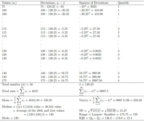
For example, Table 1 presents a synthetic data set on systolic blood pressure (in mmHg) measurements of 40 indi-viduals. The mean systolic blood pressure measurement in this example is 120.5 mmHg (see Table 1 for the calcu-lation).
Table 1. Systolic blood pressure measurements of 40 Individuals
X
erties that make it useful, especially as a measure of central tendency:
1. The mean is the only single number, for which the sum of the residuals (deviations) of each value from the estimate (the mean) is always zero. In other words, the values to the left of the mean are balanced by the values to the right of the mean. If values x1, …, xn have mean , then (x1 - ) + …+ (xn - ) =
0. Since xi - is the distance from a given number to (deviations from) the mean.
2. The mean is also the best single predictor in the sense of having the lowest root mean squared error, i.e. it minimizes error in the prediction of any one value in a given data set. In other words, if it is required to use a single value as a "typical" value for a set of known values x1, …, xn, then the mean of the values does this best,
in the sense of minimizing the sum of squared deviations from the typical value: the sum of (xi - )2.
3. The mean of a sample ( ) drawn from the population is an unbiased estimate of the population mean (µ or µx). The mean of a sample gets closer to, or converges on, the population mean as the sample size
in-crease. This property is also called the Weak Law of Large Numbers (6).
4. The mean is the most informative measure since it includes every value in the data set as part of the calcu-lation (see Equation 1).
The mean can be used with both discrete and continuous variables (interval and ratio scale), although its use is most often connected with continuous data such as age, blood pressure, body mass index (BMI), and heart rate. The mean values from ordinal scale data (such as Apgar scale, Glasgow coma score, Trauma score, and Framing-ham score) are generally misleading or invalid due to the lack of consistent level of magnitude between numeric units of the scale (7). The mean is not a useful measure when data is skewed, it will not accurately represent the data; it loses its ability to provide the best central location for the data because the skewed data is dragging it away from the "typical" value.
The mean has one main disadvantage: it is strongly influenced by outliers. Outliers are values that are unusual or extreme compared to the majority of the data points by being especially small or large in numerical value. In other words, an outlier is an observation that is numerically distant from the rest of the data (See Interquartile Range below). Outlier may be the result of measurement error, coding error, or extreme variability in an observation. It can be identified by visual inspection of the data, graphical displays, or complex modelling. Depending on the number of outliers, they are either statistically transformed (using a complex statistical formula to balance all other values) or excluded from the data set.
Arithmetic mean is a special case of weighted arithmetic mean where all values have an equal weight of one. In survey data and meta-analysis, it is common for different observations to have different weights (indicating differ-ent contributions or represdiffer-entations, some observations or samples have more weights than others). In this case, the mean calculated is called the weighted arithmetic mean (for short, the weighted mean). For example, for a set of n values x1, x2, ..., xn, with weights w1, w2, …, wn, respectively, the weighted mean is defined as:
X
X
X
X
X
Although not often used as arithmetic mean in descriptive statistics, there is another type of average or mean called the geometric mean. The geometric mean indicates the central tendency or “typical” value of a data set using the product of their values (as opposed to the arithmetic mean which uses their sum, as described above). It is defined as the nth root of the product of n numbers, for example, for a set of n values x1, x2, ..., xn, the geometric mean is
defined as:
Median
The median is the "mid-way" or central value of data that has been sorted in (ascending or descending) order of magnitude. Half the values lie below the median and half the values lie above it. It is less influenced by outliers in a data set, and more useful than the mean to describe such data sets. It is also useful for summarizing ordinal data as the magnitude of the difference between values of a data set need not be consistent to determine the median. However, it is not useful for describing nominal data such as gender or blood groups due to the arbitrary selection of numbers to denote this scale (7).
The median is a preferred measure of central tendency over the mean (or mode) when data is skewed (i.e., the fre-quency distribution for the data is non-symmetrical) or if there are one or two outliers which would make the mean unrepresentative of the majority of the data. In skewed data, unlike the mean, the median best retains its position and is not as strongly influenced by the skewed values (Figures 1A and 1C). Alternatively, geometric mean may be an appropriate summary when the distribution is positively skewed, i.e. when the most of the observations are around the centre but some on the right tail of the distributions.
If there is odd number of observations, the median is simply the middle value; if there is even number of values (n) then there is no middle one, hence the median is calculated as the average of the middle two values.
For example, for the data set in Table 1, the 40 systolic blood pressure measurements, the number of observations (n=40) is even. Hence, the median will be the [(40+1)/2]th term, i.e. the 20.5th value which is the average of the 20th
and 21st values, 20 (120+120 divided by 2 = 120) (Table 2).
Mode
The mode is the most frequent value(s) in a data set or the highest point of a peak on a frequency distribution. It is most useful to describe bi-modal distributions (when two clusters of data exist) and categorical or nominal data such as blood type (,"A", "B", "AB" and "O"), sex, race, or education level defining the most prevalent characteris-tics of a sample. The mode can also be calculated for quantitative or continuous data.
In a situation where the data is symmetrical and unimodal or does have perfect normal distribution the three meas-ures of central tendency (i.e. the mean, median and mode) are all identical (Figure 1A).
Figure 1: Density plots of different distributions. Negatively skewed (A), perfectly Normal (no skewness, B), and positively skewed (C).
Quantiles
When presenting and analyzing continuous variables, one way of categorizing observations is the use of cut-off points that classify observations into intervals where all intervals take equal proportion of the data points. These cut-off values are called quantiles (8). For example, the systolic blood pressure measurements in Table 1 can be grouped in to (a) ten equal parts using 9 deciles, (b) five classes using 4 quintiles, (c) four classes using 3 quartiles, or (d) three classes using 2 tertiles. Similarly, percentiles or centiles in short, divide a continuous variable in to hundred equal groups. The terms tertiles, quartiles, quintiles, deciles, and percentiles (or centiles) refer to the cut-off points rather than the groups obtained using these cut-cut-off values.
Quartiles are used to form four equal groups each containing 25% of the observations. In this case, only three cut-off values are required and hence, there are three quartiles (often represented as Q1, Q2, and Q3). The second
quar-tile (Q2) is known as the median since it divides the observations ordered in terms of magnitude in to two equal
halves. The lower quartile (Q1) is located one quarter of the way along the data set when the values have been
sorted in order of magnitude and the upper quartile (Q3) is located three quarters along the data set. Similarly,
Measures of Spread
A measure of spread, sometimes also called a measure of dispersion or measures of variation, is used to describe the variability that exist in a data set. It is usually used in conjunction with a measure of central tendency, such as the mean or median, to provide an overall description of a data set. Examples of measures of spread include range, interquartile range, variance and standard deviations.
Range
The range is the difference between the lowest and highest values in a data set. It the most obvious measure of variability.
It is useful for showing the spread within a data set as well as for comparing the spread between similar data set s. In the systolic blood pressure measurement (Table 1), the highest measurement is 175 and the lowest measurement is 75. Hence, the difference of these two numbers is 100, representing the range. Since range is based solely on the two most extreme values within the data set, there is a risk that it may not be representative of the variability within the data set and can sometimes be misleading. This becomes obvious if one of the two extreme values or both ex-treme values are outliers. One remedy to reduce the impact of outliers is to use inter-quartile range, which consid-ers the variability of the middle 50% of the data set.
Interquartile range
The inter-quartile range (IQR) is a measure that indicates the extent to which the central 50% of values within the data set are dispersed. It is based upon, and related to, the median or the second quartile (Q2) hence often reported
with the median as a measure of spread. The lower quartile (Q1) lies halfway between the median (Q2) and the
low-est value in the data set whilst the upper quartile (Q3) lies half way between the median (Q2) and the highest value
in the data set. The observations between the lower and upper quartiles, Q1 and Q3 constitute 50% of the total
ob-servations in the data set. The inter-quartile range is calculated by subtracting the lower quartile (Q1) from the
up-per quartile (Q3).
Quartiles and IQR are used in plotting of box and whisker plots as well as to identify outliers. In a boxplot, an outlier is often defined as a value that is located outside the fences (“whiskers") of the boxplot (e.g. outside 1.5 times the IQR above the upper quartile and below the lower quartile.
Range = Highest value - Lowest value (6)
IQR = Upper quartile (Q
3) - Lower quartile (Q
1)
(7)
80 10 0 12 0 14 0 16 0 18 0 S ys to lic _b lo od _p re ss ur e
and 126.2, respectively. The IQR is 12.4 hence the two values 75 and 175 are outside 1.5 times the IQR below the lower quartile (Q1) and above the upper quartile (Q3), respectively. Hence, both can be considered outliers in the
data set.
Variance
Variance is the average of the squared deviations (differences) of individual values from the mean. It measures how far a data set is spread out from their average value or the mean of the data set. A value of zero means that there is no variability; all the values in the data set are the same or identical hence the deviations of individual val-ues from the mean are all zero. Variance is not generally used in data description but it has a central role in statis-tics. It is used in statistical inference, hypothesis testing such as analysis of variance (ANOVA) and goodness of fit tests which will be discussed in detail in subsequent reviews in this series.
Variance is often represented by , referring to population variance and s2, referring to sample variance or Var
(X). It is calculated by squaring the deviations of each individual values from the mean, adding them together and dividing by the total number of values (n) for population variance and by n-1 (for sample variance), using the fol-lowing mathematical formulas, population variance (Equation 6) and sample variance (Equation 7):
The deviations are squared to overcome any negative deviations from the mean since it is not possible simply to average the deviations. As mentioned before, the deviations from the mean always add up to zero, the positive de-viations of values above the mean will balance out the negative dede-viations of values below the mean. Squaring the deviations, as opposed to ignoring the minus sign, also makes the summary measure mathematically tractable (3,9).
While working with the sample data, dividing the sum of deviations by (n-1) rather than n, gives a better estimate of the variance of underlying population. The n-1 in the denominator is known as the degree of freedom (df) of the variance. This is the same as the number of independent deviations (from the mean) available to estimate the vari-ance. The n deviations from the mean should add up to zero. Hence, there are only n-1 rather than n independent deviations available to calculate variance since the last one (i.e. nth deviation) can always be calculated from the rest.
A disadvantage of the variance is that it is measured in square of the units used for individual measurements. For example, in the systolic blood pressure measurements, individual units are mmHg whereas the unit if variance is mmHg2.
2
Standard deviation
The standard deviation (SD) is a measure that summarizes the amount by which every value within a data set devi-ates from the mean. It is calculated as the square root of the variance. While variance gives us a rough idea of spread, the standard deviation is more concrete, that provides average distances from the mean across all observa-tions. It is an indication of how closely the values in the data set are bunched around the mean value. The standard deviation is small when the values in a data set are bunched closely around the mean (and it is zero if all the values are equal to the mean) and large when the values are scattered over considerable distance (Figure 3).
Similar to variance, standard deviation is often represented by δ, referring to population standard deviation and s or SD, referring to sample standard deviation.
The standard deviations of n observations, sampled from a population, with means equal to is calculated us-ing the followus-ing formula:
Figure 3:Density plots of Normal distributions with the same mean ( ) but different variations (standard deviations, δ).
Table 2 shows how to calculate standard deviation and other measures of location and spread (range, interquartile range, and variance) using the example data set on systolic blood pressure measurements (in mm Hg) presented in Table 1.
X
)
(
1
1
2
X
Var
n
x
x
SD
n
i i
with the mean. Unlike the range and inter-quartile range, it takes into account every value in the data set. Unlike variance, standardized deviation is measured in the same units as the mean and, like the mean, it summarizes a great deal of information in one number and has useful mathematical properties. For example, using the standard deviation, we could tell the percentage of values or observations that are within a certain distance (standard devia-tions, SD) from the mean. For normally distributed variable, 68.26% of the observations lie within 1SD from the mean; 95.44% of the observations lie within 2 SD from the mean; and 99.7% the observations lie within 3 SD from the mean; and 95% of the observations lie between in mean-1.96 SD and mean+1.96 SD (9).
Table 2. Computing different summary measures of location and spread for the systolic blood pressure measure-ments (in mmHG) in Table 1
Standard Error of the mean (SE)
Standard error of the mean measures the average deviation of individual sample mean from the population mean. Let us assume that there is a defined population where the true population mean of a given variable, say Y, is . Let us consider all possible samples of size n (assume that there are only m possible samples of size n). For one of these possible samples, say kth sample, it is easy to calculate sample mean, . Hence, there will be one mean for each sample resulting in m different sample means for m possible samples of size n. Each of these sam-ple means is meant to serve as an estimate of the true population mean implying the need for the measure of vari-ability among these sample means taking the population mean as a reference point. This measure of varivari-ability is called standard error of the mean and calculated as follows:
It is important to distinguish standard deviation from standard error and the relationship between them. Standard deviation tells the amount of variation between observations in a given sample of size n. On the other hand, stan-dard error tells us variation between sample means obtained from all possible samples of size n generated from the same underlying population. Without requiring to take all possible samples of size n from a given population, stan-dard error can also be calculated using the SD obtained from one random sample of size n using the following
formula:
REFERENCES
1. Mann PS. Introductory Statistics (6th ed). John Wiley & Sons, 2006.
2. Trochim WM. (2006). "Descriptive statistics". Research Methods Knowledge Base. Retrieved 15 Septem-ber 2018
3. Whitley E, Ball J. Statistics review 1: Presenting and summarizing data. Critical Care 2002, 6: 143. 4. Bland J, Altman D. Transformations, means, and confidence intervals. BMJ 1996;312: 1079.
5. van Belle G, Fisher LD, Heajerty EJ, Lumley T. et al. Biostatistics: A methodology for the health sciences. Vol. 519. John Wiley & Sons, 2004.
6. Riffenburg RH . Statistics in Medicine (3rd ed). Elsevier, 2012.
7. Gaddis G, Gaddis M. Introduction to biostatistics: Part 2, descriptive statistics. Annals of Emergency Medicine 1990;19:309-315
8. Altman D, Bland J. Quartiles, quintiles, centiles, and other quantiles. BMJ 1994, 309: 996. 9. Betty R Kirkwood and Jonathan AC Sterne. Essential medical statistics. John Wiley & Sons, 2010.
y
k