R E S E A R C H A R T I C L E
Open Access
Introducing the Logarithmic finite
element method: a geometrically exact
planar Bernoulli beam element
Christian Schröppel and Jens Wackerfuß
**Correspondence: [email protected] Emmy Noether Research Group MISMO “Mechanical Instabilities in Self-similar Molecular Structures of Higher Order”, Institute of Structural Analysis, University of Kassel, Mönchebergstraße 7, 34125 Kassel, Germany
Abstract
We propose a novel finite element formulation that significantly reduces the number of degrees of freedom necessary to obtain reasonably accurate approximations of the low-frequency component of the deformation in boundary-value problems. In contrast to the standard Ritz–Galerkin approach, the shape functions are defined on a Lie algebra—the logarithmic space—of the deformation function. We construct a deformation function based on an interpolation of transformations at the nodes of the finite element. In the case of the geometrically exact planar Bernoulli beam element presented in this work, these transformation functions at the nodes are given as rotations. However, due to an intrinsic coupling between rotational and translational components of the deformation function, the formulation provides for a good approximation of the deflection of the beam, as well as of the resultant forces and moments. As both the translational and the rotational components of the deformation function are defined on the logarithmic space, we propose to refer to the novel approach as the “Logarithmic finite element method”, or “LogFE” method. Keywords: Logarithmic finite element method, Geometrically exact beam, Finite rotations, Large deformations, Lie group theory, Bernoulli kinematics
Background
We propose a novel finite element formulation, the Logarithmic finite element, or “LogFE” method, that significantly reduces the number of degrees of freedom necessary to obtain accurate approximations of boundary-value problems. The LogFE method focuses on the low-frequency part of a deformation and minimizes spurious high-frequency components in the solution.
In order to keep the exposition as simple as possible, we restrict the model presented in this paper to the case of a planar Bernoulli beam, i.e. a beam endowed with Bernoulli kinematics embedded in the Euclidean plane. In addition, we limit the degrees of freedom to coefficients related to rotations and dilatations at the nodes of the element. While we restrict the numerical examples to the evaluation of a beam consisting of one single element only, we explicitly show that degrees of freedom related to adjacent finite elements can be linked together by linear maps, based on geometrically meaningful continuity
©2016 The Author(s). This article is distributed under the terms of the Creative Commons Attribution 4.0 International License (http://creativecommons.org/licenses/by/4.0/), which permits unrestricted use, distribution, and reproduction in any medium, provided you give appropriate credit to the original author(s) and the source, provide a link to the Creative Commons license, and indicate if changes were made.
conditions. Hence, the construction of a global finite element system based on the beam elements presented in this work is possible.
Following the approach outlined in [24] and [25], we intend to present a formulation
that includes, in addition to rotations and dilatations, the translations at the nodes of the configuration in a future publication.
Interpolating on the logarithmic space
Geometrically exact beam formulations generally include both translations and rotations
as kinematic variables, following the continuum mechanics model of theelastica
devel-oped by Cosserat and Cosserat [9]. In most of the literature, the interpolation of the kine-matic variables at the integration points is performed separately for the translational and the rotational variables. Well-known deficiencies of many of these formulations, such as lack of geometric invariance, path dependence and poor accuracy in coarse meshes, have been traced back to the characteristics of the various methods proposed for the interpola-tion of the rotainterpola-tional variables by Jeleni´c and Crisfield [14] and Romero [22], among others. The modelling of beams endowed with Bernoulli kinematics within this setting presents particular challenges, especially membrane locking, as rotations and translations, although interpolated separately, must jointly satisfy the Bernoulli condition along the neutral axis. Similar difficulties characterize finite element formulations based on Lagrange functions for the axial and Hermitean functions for the transversal displacements [3,20]. As a result, the characteristics of existing finite element formulations for geometrically exact Bernoulli beams remain inferior to those available for kinematics that include shear deformations
[17]. Armero and Valverde provide an account of the historical development of
geomet-rically exact beam formulations, including a brief description of different methods that aim to eliminate or reduce the effects of the drawbacks associated with the classical beam formulations [3].
To preserve the orthogonality of the interpolated directors, a number of existing geo-metrically exact models, such as [11,14,27], identify the kinematic variables with elements
of a Lie group, the special orthogonal groupSO(3). (In the work of Ericksen and
Trues-dell, the use of the Lie group and its associated Lie algebra is implied by the differential equation given on page 306.)
In a different approach, Armero and Valverde interpolate the director frame associated with the neutral axis of the underlying geometry of a Bernoulli beam by using its angle in the plane case [3], and in the general linear groupGL(3,R) for the three-dimensional case [4]. In the latter case, orthogonality is achieved by applying a projection operator to the resulting interpolated set of vectors that preserves the direction of the vector tangent to the neutral axis, effectively resulting in an interpolation on the special orthogonal group. As the shape functions are defined not on the global coordinate system, but with regard to the local coordinate systems induced by the director frame, membrane locking is minimized due to an appropriate coupling of axial and transversal displacements. Meier, Popp and Wall extend this approach from the linear domain to large deformations, introducing an
orthogonal interpolation method based on the torsion of the neutral axis [17].
Betsch and Steinmann enforce the orthogonality of the director frame at the nodes by introducing Lagrange multipliers, thus restricting the function space of the weak form of
the equations of motion [6]. The effects of a non-orthogonal interpolation of the director
frame can be addressed by reformulating the weak form of the equations of motions in
Although the concept of the Lie group and the Lie algebra is central to the method we are proposing in the present work, we do not interpolate the kinematic variables themselves in a Lie group or in its associated Lie algebra. Instead, we aim to identify, in a function space generated by polynomial shape functions on the logarithmic space, i.e. the space of the Lie algebra, a deformation function that, in the case of the Bernoulli beam, transforms the neutral axis of the given initial configuration so as to obtain an equilibrium configuration. Choosing appropriate shape functions, both with regard to their scalar part and to their respective vector in the Lie algebra of the deformation function, is of crucial impor-tance for the performance of the proposed method. In particular, although we do not allow translations at the nodes in the present work, the vectors associated with the shape functions are not restricted to either the rotational/dilatational or the transla-tional part of the Lie algebra associated with group of planar similarity transforma-tions,sim(2,R) = (gl(1,R)⊕so(2))⊕Idt(2,R). (In this formula, Id identifies the
func-tion ϕ : g → End(n) defining the commutator of the semidirect sum of two Lie
algebras, gandn, gi ∈ g, ni ∈ n,
(g1, n1),(g2, n2)
:= (g1, n1)(g2, n2)−(g2, n2)(g1, n1),
with (g, n)(g, n) :=(gg,ϕg(n)) [14, p. 84–85] [17, p. 38–40]. For matrix Lie algebras, we
assume thatg(n)= gnis given by the matrix product). Instead, the vectors span across
the entire Lie algebrasim(2,R), inducing a strong coupling of rotational and translational kinematic variables, which results from the multiplicative group operation given as a semidirect product.
Accessible introductions to Lie group theory can be found in [13] and [17]. [2] develops formulations for the description of large rotations from elementary calculations, leading to a geometrically motivated approach to the theory of Lie groups and Lie algebras. A number of more advanced topics in Lie group theory, including the construction of semidirect products, are discussed in [26] and [16].
Interplay of rotations and translations
Due to the specific problems related to the interpolation on the group of rotations, which are not present with regard to translations, many geometrically exact formulations for finite beam elements rely on a complete separation of the rotations from the translations, e.g. [14,23,27]. This uncoupling has the obvious advantage of isolating the shape functions related to the rotations from spurious effects of the approximation of the translational part of the deformation. However, it also results in a larger number of degrees of freedom, opening up dimensions of the deformation space which are largely irrelevant in order to achieve a reasonably close approximation of the exact deformation, especially when focusing on its low-frequency component.
In contrast to the approach referred to above, which effectively is based on linear inter-polations on the Lie algebraso(3)⊕t(3,R), the direct sum of the Lie algebras associated
with the Lie groups of rotationsSO(3) and of translationsT(3,R)R3in three
dimen-sions, Sonneville, Cardona and Brüls offer a geometrically exact formulation based on the Lie algebra associated with the semidirect product of translations and rotations, i.e. the Lie algebrase(3) associated with the special Euclidean groupSE(3) :=SO(3)IdT(3,R),
the semidirect product of rotations and translations in three dimensions [28]. By
iden-tifying the local material frames, i.e. the positions and orientations of the cross-sections
of the beam along the neutral axis, with elements of the Lie groupSE(3), and linearly
translational and rotational components of the deformation. An earlier formulation that implicitly uses an interpolation of the neutral axis of a beam as well as of the orientation
of its cross-section on a the Lie algebrase(3), instead of polynomial shape functions, has
been presented by Borri and Bottasso [7]. Selig and Ding explicitly introduce Lie groups
and Lie algebras in their exposition of a screw-theoretic formulation for a planar beam
[26]. The formulations proposed in these works are ultimately based on concepts from
screw theory [5,15], also referred to as motor calculus [30,31].
To the knowledge of the authors, existing formulations for geometrically exact beam models, whether based on the Lie algebraso(n)⊕t(n,R), or on the Lie algebrase(n), for
n = 2 orn = 3, rely on a strictly linear interpolation between the degrees of freedom
given at the respective nodes (in the logarithmic space) and thus do not make use of internal degrees of freedom associated with additional shape functions, such as polynomial shape functions of higher order, that may be constructed on the Lie algebra. As a result, the image of the neutral axis of a beam element is located on an arc or a section of a helix with curvature and torsion depending exclusively on the nodal degrees of freedom. In particular, the curvature and the torsion remain constant along the neutral axis on
each beam element for both the formulation based on the special orthogonal group [22,
p. 125] as well as for the formulation based on the special Euclidean group [28, p. 460].
Due to the relatively low computational complexity of a single element, this restriction can often be compensated for by a finer discretization of the beam model. For example,
Sonneville, Cardona, and Brüls [28] achieve good convergence characteristics and small
approximation errors for a standard test case based on a bent Cantilever beam subjected to a fixed load.
However, in order to reduce the number of nodal degrees of freedom, as well as the overall number of internal and nodal degrees of freedom in the approximation algorithm, it is necessary to overcome the restriction given by a constant curvature along the neutral axis of a single beam element. In addition, by reducing the degrees of freedom, it is possible to focus on the degrees of freedom associated with the low-frequency component of the deformation while minimizing the spurious high-frequency effects. In a multigrid setting, this has the advantage of being able to separate the low-frequency component of the deformation, which is being approximated on the coarse grid, and the high-frequency part which may be approximated by a high-frequency smoothing algorithm on the fine grid.
Bernoulli kinematics rather than Timoshenko kinematics. In particular, if the orientation of the cross-section would be taken directly from the deformation function, rather than implicitly calculated from the orientation of the neutral axis, the formulation would imply the absence of shear deformation at the nodes, also for Timoshenko kinematics, a clearly non-physical result.
The deformation function
In contrast to [11,14,27], the formulation presented in this paper is based on finding a
deformation functionacting on the given initial configurationthat realizes an equilibrium
configuration of the system. It is thus thedeformation functionthat results from a function
that maps elements of the parametrization of the beam to elements of the Lie group. Thus, both the initial configuration and the current configuration are fully defined by the positions of the points along the neutral axis of the beam, with rotations obtained from the derivative of the neutral axis. As a result, in order to identify individual points on the interpolant with elements of a Lie group, one would necessarily need to take the location of the neutral axis in a neighborhood of the respective points into account.
While the interpolant of the resulting finite element contains both a rotational and a translational component, the degrees of freedom at the nodes—in the simplified variant that we describe in this work—only include rotations and dilatations (i.e. radial displace-ments with respect to a given center). Dilatational and rotational degrees of freedom determine the local dilatation and rotation in a neighborhood of the associated node, respectively, while the position of the node itself remains unchanged. The translational component on the interior of the interpolant thus arises from the impact of rotations and dilatations associated with different nodes belonging to the same finite element, as well as their interaction.
In general, the deformation functions obtained with the formulation proposed in the present work will result in current configurations that are not characterized by a constant curvature within the single finite elements, even when restricting the shape functions on the Lie algebra to linear interpolations.
Essential characteristics
The essential characteristics of the LogFE method, which distinguish it from the differ-ent approaches referenced above, can thus be summarized as follows: In the proposed formulation, the degrees of freedom, together with the shape functions, determine a multiplicative deformation functionthat is defined on the Lie group of planar similarity transformationsSim(2,R). Associating the scalar part of the shape functions with vectors thatspan across the rotational and translational subalgebrasof its associated Lie algebra induces a strong coupling of translational and rotational variables of the configuration. In
addition, it allows for the introduction of polynomial shape functions of higher order on
the logarithmic space.
shape functions can be linked by rotational values, both with each other as well as with other finite elements that accommodate continuity conditions based on rotations. Ele-ments endowed with Hermite-type shape functions may also be linked to other finite elements through common values of curvature and of the derivative of the strain at a common node. Similarly, boundary conditions may be incorporated into the set-up of a global finite element system.
Multigrid methods
Multigrid methods rely on the interplay of a smoothing algorithm on the fine grid and a general solver on the coarse grid. To obtain good convergence characteristics, the coarse grid algorithm must operate on the low-frequency part of the approximation error. At the same time, its influence on the high frequencies must be minimized. Employing a coarse grid correction that supplies, together with an approximation of the degrees of freedom, an interpolant characterized by a small high-frequency component minimized two potential difficulties that may arise in multigrid-based calculations: it can prevent the emergence of situations in which effects related to the high-frequency component of the deformation obstruct the approximation on the coarse grid, and it minimizes the risk that changes in the approximation of the high-frequency component induced by the coarse grid correction degrade the convergence characteristics of the algorithm applied on the fine grid. For a discussion of the impact of the order of the prolongation function being used to transfer the coarse grid correction to the fine grid, see [19], as well as the literature referred to in that publication.
We envisage multigrid methods as a major application of the LogFE formulation. How-ever, we have chosen not to present a complete multigrid formulation in the present paper. The model satisfies the conditions necessary for its incorporation in a multi-grid formulation as a coarse multi-grid solver, as it focuses on the low-frequency compo-nent of the deformation and allows for a straightforward calculation of the values of the degrees of freedom on the fine grid from the interpolant on the coarse grid. We therefore leave the practical implementation of the LogFE model in a multigrid context to future research.
Outline of the paper
Some aspects more closely related to the implementation of the method have been included in the appendices. Appendix 1 outlines how LogFE element formulations adjusted for given boundary conditions can be constructed. Appendix 2 presents a sharp upper bound for the absolute value of the error of an approximate solution for the deriv-ative of the matrix exponential.
Methods
Kinematics
The basic concepts of the LogFE model can be used to develop formulations for different classes of finite elements. However, in order to keep the exposition as simple as possi-ble, and in order to focus on the essential aspects of the model, we restrict the following description of the LogFE model to the example of large deformations of a prismatic beam in the Euclidean plane with rectangular cross-section, endowed with Bernoulli kinemat-ics. In addition, we limit the degrees of freedom to coefficients related to rotations and dilatations at the nodes of the element. The beam is assumed to consist of a homoge-neous, isotropic material. The beam model can be classified as a geometrically exact beam formulation for finite rotations.
The deformation function
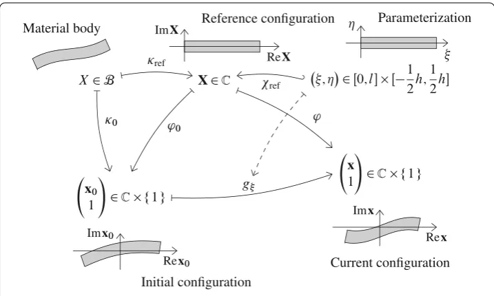
The continuous body B, which is composed of the particles X of the beam, is given
as a domain in a topological space (see Fig.1). After placing the particles of the beam
in the reference configuration, we discretize the beam into finite elements and endow the elements with a parametrization, such that set of particles of the beam along the codimension of the parameterization (i.e. the width) can be unambiguously identified with a tuple of parameterizing variables (ξ,η)∈R2. The variableξ determines the location of the cross-section containing a given material point of the beam along the neutral axis. As a result of assuming Bernoulli kinematics, the position and orientation of the points in a
given cross-section of the beam are fully determined by the location and the orientation of the neutral axis.
The location of a material point in the reference configuration is given byX=κref(X),
withκref mapping the domainBcontinuously into the Euclidean plane, which we will,
after choosing an arbitrary origin, identify with the complex plane. This identification serves two purposes: it simplifies the notation, and it immediately clarifies, by the use
of complex numbers instead of matrices representing linear maps on R2, that, within
this work, all linear maps operating onR2are restricted to the commutative subgroup
GL(1,R)×SO(2)GL(1,C) of the general linear groupGL(2,R) given by the dilatations and rotations. In particular, the deformation functiongξ(see Fig.1), as a function of the degrees of freedom, assumes values that can be represented by matrices with complex entries.
We discretize the beam as a single finite element. The parameterization, a Lipschitz continuous embedding, maps into the reference configuration according to the function
χref : [0, l]×
−1
2h,12h
→C, (ξ,η)→ξ+iη, (1)
in whichlandhdenote the length and the height of the beam, respectively.
In order to express both rotations and translations as a single, multiplicative operation,
we will use the concept of homogeneous coordinates. By placing a vector spaceV into a
larger constructV×{1}, we can express the translation of a vector inVas a multiplication of an element ofV× {1}by a matrix. Givenv0,v∈V,R∈GL(V), we have
Rv0+v
Rv0
1
+
v 1
=
R v0
0 1
v 1
. (2)
Expressing both linear maps and translations in this way also allows us to describe the
logarithm of the functionv0 →Rv0+v, as the logarithm of the matrix
R v 0 1
. The
logarithm plays an essential role in the theory of Lie groups and Lie algebras, on which the LogFE method is based. It is given as the (generally multi-valued) inverse of the exponential function, which is defined as exp(•) :=∞k=0k1!•k. In this definition, the symbol “•” may denote a scalar, a matrix, or a function. In the case of a function, taking thekth power is
defined as consecutively applying the function for a total ofktimes.
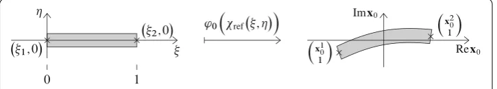
We therefore embed both the initial configuration,x0, and the current configuration,
x, into the homogenized Euclidean planeE2× {1}, which we identify withC× {1}.
Fig-ure 2 illustrates the map from the parametrization space into the space of the initial
configuration.
The motion of the body from the initial configuration to the current configuration
is given by a continuous mapg(ξ) which depends on the parameter ξ and acts on the
initial configuration, i.e. on
x0
1
=ϕ0(X)=ϕ0(χref(ξ,η)). A point x in the current
configuration is given by
x 1
=gξ
x0
1
=gξ(ϕ0(X))=gξ(ϕ0(χref(ξ,η))). (3)
For points of the neutral axis, we haveη≡0, thus their position in the current
configu-ration only depends on the parameterξ. The mapg(ξ) depends on the parameterization
variableξ, but acts on the space of the initial configuration, i.e. onC× {1}.
Lie groups and Lie algebras
All functionsg(ξ) are given in the form exp ( ¯Z(ξ)) and act on elements ofC× {1}. ¯Z(ξ) is an element of a Lie algebra and is therefore endowed with specific properties. We recall some basic results from the theory of Lie groups and Lie algebras, which are relevant for the subsequent formulation of the model.
Members of a set form a group, denotedG, if there exists an associative binary operation
G×G→G, there exists a neutral elemente∈ Gwith regard to this operation, and for
every elementg ∈Gthere is an inverse elementgsuch thatgg =e.
The values of the functiong(ξ) are elements of the subgroup
a b
0 1 a∈C\ {0}, b∈C
(4)
of the 2 ×2 matrices over the complex numbers. They form a group with regard to
the multiplication, which we will also denote G. The identity map, denoted Id, is the
neutral element of G. While this group can be embedded in the general linear group
GL(2,C), as shown in Eq. (4), a more concise description characterizes this Lie group of the valuesg(ξ) as the group of complex similarity transformationsSim(1,C)=GL(1,C)Id T(1,C), which is isomorphic to the group of planar similarity transformationsSim(2,R)= (GL(1,R)×SO(2))IdT(2,R), with the group action defined as (s, R, t)◦
s, R, t =
ss, RR, sRt+t,SO(2) being the special planar orthogonal group. With regard to these operations,sis a scaling parameter,Ris a rotation matrix, andtis a translation vector. The action of this Lie group on a vector in the Euclidean space is defined bys, R, t◦x=sRx+t,
with x ∈ R2. For the isomorphic complex Lie group, the group operation is given as
(a, b)◦a, b=aa, ab+b, and the action on a vector space as (a, b)◦z=az+b, with
z ∈C. As these group operations indicate, calculations on a Lie group generally do not
involve multiplications of complete matrices, although many Lie groups, including those referred to in this work, can be embedded in the general linear group, thus facilitating the understanding of the group action and the action of the group on a vector space.
Each element of the group can be obtained by taking the exponential of an element ¯Z(ξ). Furthermore, exptZ¯(ξ)∈ Gfor allt ∈ R. Therefore,Gis a Lie group, and the set of elements ¯Z(ξ) forms the Lie algebra ofG, denotedg.
As a Lie algebra,gis a vector space together with the adjoint map, a skew-symmetric
commutatorof the Lie algebra. The specific Lie algebra that will be used in the remainder of the text,g:=sim(1,C)=gl(1,C)Idt(1,C), can be represented by the matrices
a b
0 0 a∈C, b∈C
. (5)
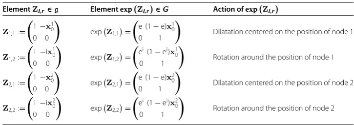
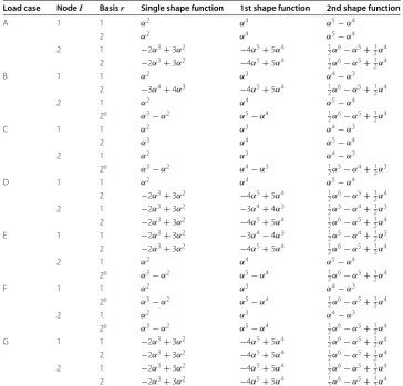
In particular, it contains the elementsZI,r given in Table1. As will be described below
in more detail, each element is associated with one or more shape functions. The index
I designates the node associated with the shape functions constructed from the element
ZI,r, whiler, which can assume the values 1 or 2, denotes the type of the deformation. The
caser = 1 indicates that the shape function characterizes a dilatation with the position
of the nodeIas its fixed point, whiler=2 indicates a rotation around the position of the
nodeI. By the term “dilatation”, we refer to a radial displacement of the material points
with regard to a given center, the fixed point of the deformation. A dilatation thus induces volumetric strain in the body.
Each of the elementsZI,r generate a subalgebra ofg. We also note that ZI,1 andZI,2
are independent vectors ofg, understood as a vector space. ForλI,1,λI,2∈R, the element
exp ( ¯ZI)∈G, with ¯ZI=λI,1ZI,1+λI,2ZI,2, represents the action of simultaneously rotating
and dilatating the initial configuration, with the positionxI0of the nodeIas the invariant
point. The exponential of a linear combination of the elementsZI,rrepresents a mixture of
their respective actions on the initial configuration whose invariant point generally does not coincide with the position of either node.
A parameterized curve on the Lie algebra, seen as a vector space, can be given by
γ(ξ) :=
1≤I≤nel 1≤r≤2
λI,r(ξ)ZI,r, (6)
withγ(ξ)∈g. In this equation,nel denotes the number of nodes per element. For each
locationξ, the curveγ(ξ) determines the map expγ(ξ)∈G, that will be applied to the
material points of the initial configuration associated withξ. In particular, as every node
I is associated with a specific valueξIof the parameterization variable,γ(ξ) provides an interpolation of the transformation applied to the respective nodes.
Shape functions
In the following, we will construct the shape functions for a finite beam element consisting
of two nodes, i.e.nel=2. Both nodes are located on the neutral axis. The coordinates of
Table 1 Elements of the Lie algebragand the associated Lie groupG
ElementZI,r∈g ElementexpZI,r∈G Action ofexpZI,r
Z1,1:=
1−x1 0 0 0
expZ1,1
=
e (1−e)x1 0
0 1
Dilatation centered on the position of node 1
Z1,2:=
i−ix10 0 0
expZ1,2=
ei(1−ei)x10
0 1
Rotation around the position of node 1
Z2,1:=
1−x20 0 0
expZ2,1=
e (1−e)x20
0 1
Dilatation centered on the position of node 2
Z2,2:=
i−ix2 0 0 0
expZ2,2=
ei(1−ei)x2 0
0 1
the locations of the node with indexIare given as (ξI,0). We define the functiong(ξ) in Eq. (3) as
gξ:=expZ¯(ξ)=exp ⎛ ⎜ ⎜ ⎜ ⎜ ⎜ ⎝
1≤I≤nel 1≤r≤2 0≤q≤nq−1
uI,r,q
NI,r,q(ξ)
pI,r,q(ψI(ξ))ZI,r
NI,r,q(ξ)
⎞ ⎟ ⎟ ⎟ ⎟ ⎟ ⎠
, (7)
In this equation,rdenotes the index of the respective element of the Lie algebra, andnq
denotes the number of polynomial functionspI,r,q that are being used to construct the
shape functionsNI,r,q(ξ) related to an elementZI,r of the the Lie algebrag, such that, for a given nodeI,ZI,r are linearly independent.NI,r,q(ξ) may be understood as the scalar part of the shape function, determining the “intensity” of the deformation, while its basic characteristics (dilatation/rotation, invariant point) are given byZI,r. The termZI,rin Eq. (7) is generally not present in conventional finite element models, in which shape functions are understood as translations defined by the scalar valueN(ξ) and a basis vectorei, and are defined separately for each dimension in the vector space of the configuration. In such formulations, a coordinate-based description if often used, thus dropping the basis vectorei. In the context of the beam model described, we havenel = 2,r ∈ {1,2}, and nq≥1.ψI(ξ) are the barycentric coordinates constructed on the interval=[ξ1,ξ2] and
associated with the nodeI. The function ¯Z(ξ) thus is Lipschitz continuous, differentiable
and bounded on.
Continuity conditions
All numerical calculations in this work are restricted to dilatations and rotations at the nodes. It is, however, natural to ask whether the model can, in principle, be extended to a formulation including translations, and whether it is possible, based on that formulation, to perform numerical simulations not just for a single finite element, but for a complete finite element system, by applying standard procedures of the finite element on the global level. In order to be able to answer these questions in the affirmative, we show
(1) that the formulation presented here is indeed a special case of an extended formula-tion that includes translaformula-tions, and
(2) that the extended formulation, given suitable shape functions, results, in a sufficiently large domain of the space of the degrees of freedom, in a completely additively sepa-rable linear isomorphism (i.e., a one-to-one correspondence with possibly different proportionality factors) between the degrees of freedom and certain functionals of the interpolant which can be used as continuity conditions. This condition corre-sponds to the third criterion for finite elements as given by Ciarlet in [8, p. 78–9].
Preliminary considerations
In addition to the Lie groupG, we are considering the Lie group ˜G, and show that the
application of ˜G, together with a suitable set of embeddings and projections, results in the
same deformation function as the application of the Lie algebraGwith the embeddings
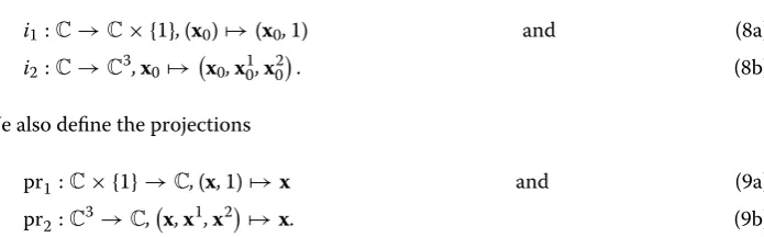
i1:C→C× {1},(x0)→(x0,1) and (8a)
i2:C→C3,x0→
x0,x01,x02
. (8b)
We also define the projections
pr1:C× {1} →C,(x,1)→x and (9a)
pr2:C3→C,x,x1,x2→x. (9b)
Table2shows the generators of the Lie algebra ˜g, as well as their exponentials, which are elements of the Lie group ˜G.
We note that the Lie algebra ˜gcan be extended to a larger Lie algebras:=g˜⊕Idt(3,C),
which includes translations. Table3shows the bases of the vector space of the Lie algebra
t(3,C)=t1⊕t2⊕t3and their respective exponentials.
For matrix Lie algebras, the multiplication is given by the canonical matrix
multipli-cation, and thecommutator [X, Y] is defined as [X, Y] := XY −YX. A Lie algebragis
calledabelianif its commutator vanishes identically, i.e. if [X, Y] = 0for allX, Y ∈ g.
If a Lie algebragis abelian, then the elements of its associated Lie group commute, i.e.
forX, Y ∈ g, we have eXeY = eYeX and therefore eXeY = eX+Y. We note that the Lie algebra ˜ghas the abelian subalgebras ˜g1and ˜g2, giving rise to their respective commutative
Lie groupsG1andG2, and that the Lie algebrass1 := g˜1⊕Idt1ands2:= g˜2⊕Idt2are
abelian and constitute subalgebras of the Lie algebras. Neither of the Lie algebras ˜gand s, however, is abelian.
Table 2 Elements of the Lie algebrag˜and the associated Lie groupG˜
ElementZ˜I,r∈g˜ ElementexpZ˜I,r∈G˜ Subalgebra ing˜
˜ Z1,r:=
⎛ ⎜ ⎝
z1,r −z1,r 0
0 0 0
0 0 0
⎞ ⎟
⎠ expZ1˜ ,r=
⎛ ⎜ ⎝
expz1,r1−expz1,r0
0 1 0
0 0 1
⎞ ⎟
⎠ g˜1= Z1˜ ,r,r∈ {1,2}
˜ Z2,r:=
⎛ ⎜ ⎝
z2,r 0−z2,r
0 0 0 0 0 0
⎞ ⎟
⎠ expZ2˜ ,r=
⎛ ⎜ ⎝
expz2,r0 1−expz2,r
0 1 0
0 0 1
⎞ ⎟
⎠ g˜2= Z2˜ ,r,r∈ {1,2}
zI,rassumes the following values:z1,1=z2,1=1,z1,2=z2,2=i
Table 3 Elements of the Lie algebratand the associated Lie groupT
ElementTI,r∈t(3,C) ElementexpTI,r∈T(3,C) Subalgebra int(3,C)
T1,r:=
⎛ ⎜ ⎝
t1,r
t1,r
0
⎞ ⎟
⎠ expT1,r=
⎛ ⎜ ⎝
t1,r
t1,r
0
⎞ ⎟
⎠ t1= T1,r,r∈ {1,2}
T2,r:=
⎛ ⎜ ⎝
t2,r
0 t2,r
⎞ ⎟
⎠ expT2,r=
⎛ ⎜ ⎝
t2,r
0 t2,r
⎞ ⎟
⎠ t2= T2,r,r∈ {1,2}
T3,r:=
⎛ ⎜ ⎝
t3,r
0 0
⎞ ⎟
⎠ expT3,r=
⎛ ⎜ ⎝
t3,r
0 0
⎞ ⎟
⎠ t3= T3,r,r∈ {1,2}
Thus, at the border of a finite element, the deformation function assumes values belong-ing to commutative subgroups of the Lie group ˜G, while its values in the interior of a finite element generally do not commute. It is this property, arising from the specific embedding of the two abelian subalgebras into a larger Lie algebra, in which the interpolation takes place, that results in a strong coupling of rotational and translational components of the deformation function in the interior of a finite element, while preserving the separability of the components on its borders.
In future work, we intend to demonstrate that most of the steps in the subsequent calculations can be readily applied to deformation functions based on the larger Lie algebra s, which includes the translational Lie algebrat(3,C). In order to keep the calculations as simple as possible, however, we restrict the following exposition to the case of rotations and dilations, i.e. to a deformation function based on the Lie algebra ˜g. In this context, we note that our current research on a model involving translations has shown that in order to obtain good approximations of solutions involving large, simultaneous translations and rotations, the application of a co-rotational approach is necessary. The restricted model presented in the subsequent exposition, however, can be formulated without that additional layer of complexity.
For a given value ofξ, the deformation functiongξis an element of the Lie groupG. Given
the valuesNI,r,q(ξ) of the shape functions at the positionξ and the degrees of freedom
uI,r,q, which may be assembled into a vector of d.o.f.u ∈ U R4nq, the deformation function results from the application of the map
ψ1:U→C1(R,g), u→ϕ1:R→g, ξ →
1≤I≤nel 1≤r≤2 0≤q≤nq−1
uI,r,qNI,r,q(ξ)ZI,r, (10)
followed by subsequent exponentiation. Similarly, a deformation function ˜gξresults from
the map
ψ2:U→C1(R,g˜), u→ϕ2:R→g˜, ξ →
1≤I≤nel 1≤r≤2 0≤q≤nq−1
uI,r,qNI,r,q(ξ) ˜ZI,r, (11)
and subsequent exponentiation. By elementary calculations, it can be shown that, for identical shape functions NI,r,q(ξ) and initial configurationx0(ξ,η), the results of the
action ofgξ := exp (ψ1(u)(ξ)) and ˜gξ := exp (ψ2(u)(ξ)) on the respective embeddingsi1
resp.i2of the initial configuration result in the same current configuration [25]. That is,
we have
x(ξ,η)≡pr1◦exp (ψ1(u)(ξ))
=gξ
◦i1◦x0(ξ,η)≡pr2◦exp (ψ2(u)(ξ))
=g˜ξ
◦i2◦x0(ξ,η) (12)
for everyx0and everyu. The calculations are available from the authors upon request.
other than by the condition that it be an immersion of the parametrization space into the physical space. Without loss of generality, we assume, in the remainder of this section, that the first node of the beam element is located at the origin, i.e.x0(0,0)=0.
Conditions related to the first derivative of the deformation function
Due to the underlying Bernoulli kinematics, the orientation of the cross-section depends solely on the orientation of the neutral axis of the beam. We also note that, as a result of the application of constitutive equations for beams with invariant cross-sections, the dilatational component of the deformation of the cross-section implied by the construc-tion of the deformaconstruc-tion funcconstruc-tion does not enter into the evaluaconstruc-tion of the internal energy.
The derivative of the current configurationxwith regard to the parameterization variable
of the neutral axis,ξ, is given by
∂x
∂ξ(ξ,η)=pr2◦
∂exp (ψ2(u))
∂ξ (ξ)◦i2◦x0(ξ,η)
+pr2◦exp (ψ2(u)(ξ))◦i2◦ ∂x0
∂ξ (ξ,η), (13)
Given an appropriate choice of shape functionsNI,r,q(ξ), this equation can be reduced
to a much simpler expression. In particular, we will impose the following restrictions on the basis functions:
NI,r,q(0)=0 for nodes and indices (I, q)=(1,0), (14a)
NI,r,q(0)=0 for all nodesIand indicesq,except for (I, q)=(1,0), (14b)
∂NI,r,q
∂ξ (0)=0 for nodeI=2. (14c)
With regard to the derivative of the exponential of a matrix-valued function, we note that for a differentiable functionX(t) :R→h, whose codomain is the Lie algebrah, we have
∂eX(t) ∂t (t
∗)=eX(t∗)∞
k=0
(−1)k (k+1)!adX(t∗)
k∂X
∂t (t
∗). (15)
This equation results from transforming the fractional expression involving the exponen-tial of the adjoint map given in [13, p. 71],
∂eX(t)
∂t (t
∗)=eX(t∗)ad X(t∗)−1
I−exp−adX(t∗) ∂
X ∂t (t
∗), (16)
into a power series. In this equation, we use the adjoint operator ad, which, forX, Y ∈h,
is given by
ad :h→GL(h), X→adX :h→h, Y →[X, Y], (17)
where [X, Y] is the commutator as defined above. Furthermore, adXkdenotes the repeated
application of adX. Thus, ifXandY are elements of a Lie algebrah, the power series in
(15), as well as the sum of any subset of its summands, evaluates to an element ofh. In
particular, ifhis an abelian Lie algebra, then Eq. (15) simplifies to
∂eX(t)
∂t (t
∗)=eX(t∗)∂X ∂t(t
∗). (18)
Given the restrictions in (14), we observe thatψ2(u)(0)∈g˜1,∂ ψ∂ξ2(u)(0)∈g˜1, and therefore,
∂exp (ψ2(u))
∂ξ (0)=exp (ψ2(u)(0))
∂ ψ2(u)
∂ξ (0). (19)
Asx0(0,0)=0andx10=0, forξ =0, the first summand in Eq. (13) is of the form
pr2◦ ⎛ ⎜ ⎝
z −z 0
0 0 0
0 0 0
⎞ ⎟ ⎠
⎛ ⎜ ⎝ 0 0 x20
⎞ ⎟
⎠, (20)
withz∈C, and thus vanishes. Given the restriction (14b), the remaining terms in Eq. (13) simplify to
∂x
∂ξ(0,0)=exp
⎛
⎝
1≤r≤2
u1,r,0N1,r,0(0)z1,r ⎞ ⎠◦∂x0
∂ξ (0,0), (21)
Withxξ= ∂∂ξx,x0ξ = ∂
x0
∂ξ , the main branch of the logarithm of the directional derivative of the deformation function, Log◦∂∂xxξ
0ξ(0,0)=
1≤r≤2u1,r,0N1,r,0(0)z1,r, a (nonlinear) func-tional of the deformation function, is an element of the Lie algebrag1and, asN1,r,0(0)=0
forr ∈ {1,2}due to condition (14a), depends linearly on the degrees of freedomu1,r,0, r∈ {1,2}in a neighborhoodUof the origin. We note thatUis a strip of width 2πin the
space of the degrees of freedomU, due to the ambiguous nature of the logarithm function.
Thus, inU, there is a one-to-one relationship between the parametersu1,r,0in the
defor-mation function of a single finite element and the respective functional of the defordefor-mation function at the border of the finite element. Therefore, by defining continuity conditions based on these functionals, the respective parameters can be linked together at the global level and thus serve as global degrees of freedom of a finite element system composed of LogFE-based finite elements, as well as other compatible finite elements.
Conditions related to the second derivative of the deformation function
If one intends to use not only the first derivative of the current configuration w.r.t. the para-meterization of the neutral axis, but also its second derivative, then additional restrictions must be imposed on the shape functions. We impose the following additions restrictions on the shape functions:
∂NI,r,q
∂ξ (0)=0 for nodes and indices (I, q)=(1,1), (22a)
∂NI,r,q
∂ξ (0)=0 for all nodesIand indicesq,except for (I, q)=(1,1), (22b)
∂2N I,r,q
∂ξ2 (0)=0 for nodeI=2. (22c)
The second derivative of the current configuration w.r.t. the parameterization of the neutral axis is given by
∂2x
∂ξ2(ξ,η)=pr2◦
∂2exp(ψ 2(u))
∂ξ2 (ξ)◦i2◦x0(ξ,η)
+2pr2◦∂exp(ψ2(u))
∂ξ (ξ)◦i2◦
∂x0(ξ,η) ∂ξ
+pr2◦exp(ψ2(u)(ξ))◦i2◦∂ 2x
0
With restriction (22c), we have∂2ψ2(u)
∂ξ2 (0)∈ g˜1and thus,∂
2exp(ψ2(u))
∂ξ2 (0)∈g˜1. As for the first derivative, the first summand in Eq. (23) vanishes forξ =0, i.e. pr2◦∂2exp(ψ2(u))
∂ξ2 (0)◦ i2◦x0(0,0)=0. With restriction (22b), we obtain
∂2x
∂ξ2(0,0)=2pr2◦
∂exp (ψ2(u))
∂ξ (0)◦i2◦∂
x0
∂ξ (0,0)
+pr2◦exp (ψ2(u))(0)◦i2◦∂ 2x
0 ∂ξ2(0,0)
=pr2◦exp (ψ2(u)(0))
2∂ ψ2(u)
∂ξ (0)◦i2◦ ∂x0
∂ξ (0,0)+i2◦ ∂2x
0 ∂ξ2(0,0)
= ∂xξ
∂x0ξ
(0,0) ⎛
⎝2
1≤r≤2
u1,r,1∂ N1,r,1
∂ξ (0)z1,r
∂
x0
∂ξ (0,0)+ ∂2x
0 ∂ξ2(0,0)
⎞ ⎠.
(24)
Based on the well-known definitions of the (geometric) curvatureκof the current
config-uration andκ0of the initial configuration, we define the “material curvature”κmatof the
current configuration andκ0matof the initial configuration of the neutral axis, as
κmat:= |∂ξx|
|∂ξX|κ =
|∂ξx×∂ξ2x|
|∂ξx|2|∂ξX|, κ mat 0 :=
|∂ξx0|
|∂ξX|κ0=
|∂ξx0×∂ξ2x0|
|∂ξx0|2|∂ξX|
. (25)
We denotes:= ∂∂xxξ
0ξ(0,0)∈C. Then, by inserting the derivatives from Eqs. (13) and (24), followed by elementary calculations, we obtain
κmat(0,0)=
|s|22Im
1≤r≤2u1,r,1∂ξN1,r,1(0)z1,r
|∂ξx0(0,0)|2+ |∂ξx0(0,0)×∂ξ2x0(0,0)|
|s|2|∂ξx
0(0,0)|2|∂ξX(0,0)|
=2u1,1,1∂ξN1,1,1(0)
|∂ξX(0,0)| +κ
mat
0 . (26)
Therefore, the change in the material curvature of the current configuration relative to the initial configuration is a linear function in the degree of freedomu1,1,1, and condition
(22a) ensures that this function is non-trivial. Obviously, care must be taken to ensure that different finite elements, which may not have the same parameterization with regard to their material points, are linked through appropriately formulated continuity conditions w.r.t. their material curvature.
We define the “material derivative of strain” ˙εmatof the current configuration and ˙εmat0 of the initial configuration of the neutral axis, as
˙
εmat =
∂ξx,∂ξ2x
|∂ξx|2|∂ξX|, ε˙
mat 0 =
∂ξx0,∂ξ2x0
|∂ξx0|2|∂ξX|
. (27)
An elementary calculation similar to that performed in Eq. (26) yields
˙
εmat(0,0)=2u1,0,1∂ξN1,0,1(0)
|∂ξX(0,0)| +˙ε
mat
0 (0,0). (28)
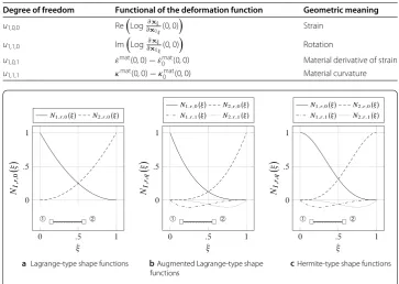
The choice of shape functions
Table4summarizes the degrees of freedom, their respective functionals, which may be
used to impose continuity conditions at the global level, and their respective geometric meaning.
A set of shape functions that satisfies the conditions (14) and (22) and thus
accommo-dates the application of continuity conditions both with regard to the first and the second derivative of the deformation function, generally does not generate the same deformation space as a set of shape functions that satisfies none or only some of these conditions, and may also have inferior numerical properties. Therefore, the optimal choice of shape functions for a finite element constructed on the basis of the Logarithmic finite element method will depend on the presence of continuity conditions and boundary conditions at its borders.
For a beam element endowed with one shape function per nodeIand Lie algebra
ele-ment ZI,r (Lagrange-type shape functions), the polynomialspI,r,0 : α → α2 therefore
satisfy the conditions (14). For the case of two shape functions per nodeIand Lie algebra
elementZI,r(augmented Lagrange-type shape functions), the polynomialspI,r,0:α→α3
andpI,r,1:α→α4−α3satisfy these conditions. Figure3displays the Lagrange-type and
augmented Lagrange-type shape functions for a two-node beam element. Note that both
sets of Langrangian-type shape functions (see Fig.3) do not satisfy the additional
condi-tions (22), and therefore cannot be used to model finite elements subjected to continuity
conditions or boundary conditions involving the second derivative of the deformation
function. However, the Hermite-type shape functions (see Fig.3) satisfy both sets of
con-Table 4 Degrees of freedom and related functionals of the deformation function, for node 1 withx10=x0(0,0), and shape functions satisfying conditions (14) and (22)
Degree of freedom Functional of the deformation function Geometric meaning
u1,0,0 Re
Log∂∂xxξ 0ξ(0,0)
Strain
u1,1,0 Im
Log∂∂xxξ 0ξ(0,0)
Rotation
u1,0,1 ε˙mat(0,0)−ε˙mat0 (0,0) Material derivative of strain u1,1,1 κmat(0,0)−κ0mat(0,0) Material curvature
a Lagrange-type shape functions bAugmented Lagrange-type shape c
functions
Hermite-type shape functions
Fig. 3 Polynomials of the shape functions for a two-node beam element. The scalar shape functionsNI,r,q
ditions and can therefore be used to construct finite elements that can accommodate all
types of continuity and boundary conditions described above (see Table4). The choice of
appropriate shape functions for different boundary conditions is discussed in more detail in Appendix 1.
Consistency with the linear beam theory
A non-linear boundary-value problem is often solved by iteratively obtaining the solutions of a sequence of linear problems, obtaining a sequence of solutions that converges toward the non-linear solution. In this section, we therefore investigate in more detail the linear steps involved in the iterative process of finding a non-linear solution. In particular, we focus on the initial linear step, for which the initial estimate for the degrees of freedom is given by the zero vector, i.e. the initial estimate for the deformation function is the identity function. We will compare the characteristics of this initial linear step with the linear theory of the Bernoulli beam. We will see that for certain standard load cases, the reaction of the beam in a neighborhood of the identity deformation predicted by the linearization of the LogFE model is identical, up to terms of higher order, to the reaction predicted by the linear theory of the Bernoulli beam.
The linearization of the LogFE formulation around the origin, i.e.u = 0, results in a
simplified model that can be regarded as a linear variant of the general approach. In this case, the degrees of freedom assume values that are proportional to the load intensity. As a result, the trajectories of the materials points of the configuration are located on the orbits of their initial locations under the action of a one-parameter Lie group. As we will see, these orbits are located on circles (and straight lines, which can be regarded as degenerate circles) if the dilatation coefficients vanish. In the case of non-zero dilatation coefficients, the orbits are located on logarithmic spirals. In order to analytically determine the linearization for different load cases, the strain and the curvature (and, as a result, the
normal force and the bending moment) at a given parameter valueξof the configuration
must be derived from the deformation function.
Normal force and bending moment
The neutral axis of the beam shall be parameterized by the curve
ξ →χ0(f (ξ))=
ξ
1
,
connecting the nodal positionsx10=0 andx20=1 on a straight line on the real axis. Thus,
we havex0(ξ)= ξ. In the following, the scalar product and the determinant are based
on the Euclidean vectors associated with the complex values, i.e. forw, z∈C, we have, in
this context, the scalar product
w, z:=
Re (w) Im (w)
,
Re (z) Im (z)
and the determinant
|w, z|:=det
Re (w) Re (z) Im (w) Im (z)
.
With ˙x:=∂ξx, ¨x:=∂2
ξx, the strainεis given asε(ξ)= x˙ −1 and the curvatureκis given asκ(ξ)= x˙−3|x˙,x¨|. The derivatives with respect to a given degree of freedomu are
∂uε(ξ)= x˙−1∂ux˙,x˙ and (29a)
∂uκ(ξ)= −3x˙−5∂ux˙,x˙ |x˙,x¨| + x˙−3(|∂ux˙,x¨| + |x˙,∂ux¨|). (29b)
Thus, forx˙ =1,x¨ =0, we obtain the derivative of the strain as∂uε(ξ)= ∂ux˙,x˙and the derivative of the curvature as∂uκ(ξ)= |x˙,∂ux¨|. Foru=0, we have ¯Z(ξ)≡0,eZ¯(ξ)≡ Id, from which follows∂uZ¯(ξ),Z¯(ξ)
≡0and therefore∂ueZ¯(ξ)≡∂uZ¯(ξ). We obtain
˙
x=∂ξeZ¯(ξ)
x0(ξ)
1
+eZ¯(ξ) 1 0 = 1 0 , (30a)
∂ux˙=∂u∂ξZ¯(ξ)
x0(ξ)
1
+∂uZ¯(ξ)
1 0
, (30b)
∂ux¨=∂u∂ξ2Z¯(ξ)
x0(ξ)
1
+2∂u∂ξZ¯(ξ)
1 0
. (30c)
Thus, the derivatives of the strain and the curvature are given by
∂uε(ξ)=
∂u∂ξZ¯(ξ)
x0(ξ)
1
+∂uZ¯(ξ) 1 0 , 1 0 and (31a)
∂uκ(ξ)= 1 0
,∂u∂ξ2Z¯(ξ)
x0(ξ)
1
+2∂u∂ξZ¯(ξ) 1 0 , (31b)
respectively. Withη1= 1 (dilatation),η2= i (rotation), the elements of the Lie algebra
are given as ZI,r,q = ηr
1 −xI0
0 0
. For the derivatives of the strain and the curvature
with respect to the degrees of freedomu, evaluated atu=0, we therefore obtain
∂uI,r,qε(ξ)=Re
ηr
∂ξNI,r,q(ξ)
x0(ξ)−xI0
+NI,r,q(ξ)
and (32a)
∂uI,r,qκ(ξ)=Im
ηr
∂2
ξNI,r,q(ξ)
x0(ξ)−x0I
+2∂ξNI,r,q(ξ)
. (32b)
Equations (32a) and (32b) indicate that the linearized strain depends on the dilatation coef-ficients only, while the linearized curvature depends solely on the rotation coefficients. For a two-node, simply supported beam element without internal degrees of freedom, i.e.
¯
QI =0, the differentials of the strain and of the curvature at the origin are given by
dε(ξ)=
I∈{1,2}
∂ξNI,1,0(ξ)
x0(ξ)−xI0
+NI,1,0(ξ)
duI,1,0, (33a)
dκ(ξ)=
I∈{1,2}
∂2
ξNI,2,0(ξ)
x0(ξ)−x0I
+2∂ξNI,2,0(ξ)
Linearization based on rotation coefficients
For a simply supported beam, subjected to an external momentM0at node 1, we have
N1,2,0(ξ)=p1,2,0(ψ1(ξ))=(1−ξ)3= −ξ3+3ξ2−3ξ+1, (34)
N2,2,0(ξ)=p2,2,0(ψ2(ξ))= −2ξ3+3ξ2. (35)
Therefore,
dκ(ξ)=ϕ1(ξ) du1,2,0+ϕ2(ξ) du2,2,0, (36)
with
ϕ1(ξ)= −12ξ2+18ξ−6, (37a)
ϕ2(ξ)= −24ξ2+30ξ−6. (37b)
If the rotation coefficients are set to zero, i.e.u1,1,1=0,u2,1,1=0, the linearized strain
van-ishes, asη2=i and therefore, as a result of Eq.32a,∂uε(ξ)=0. A linearization of the total energyUat the initial configuration, with vanishing initial curvatureκ0(ξ)≡0, is given by
U = 1 2EI
1
0 κ
(ξ)2 ∂ξx0 dξ−M0u1,2,0, (38)
with κ(ξ) = (ϕ1(ξ)u1,2,0 + ϕ2(ξ)u2,2,0)m−1. The equilibrium condition is given by ∂u1,2,0U = 0 for allI, resulting inu1,2,0 =
1
3(EI)−1M0m, u2,2,0 = −16(EI)−1M0m. With
these values, the curvature is given byκ(ξ)=(ξ −1)(EI)−1M0. These results are
consis-tent with the linear theory of the Bernoulli beam.
In a finite element formulation based on the LogFE method, the function
g0(ξ) (x0(ξ))=exp
⎛ ⎜
⎝
I,q sβI,2,q =uI,2,q
NI,2,q(ξ)ZI,2,q ⎞ ⎟ ⎠x0(ξ)
=esexp
I,qβI,2,qNI,2,q(ξ)ZI,2,q
˜
Z(ξ)
x0(ξ), (39)
withI∈ {1,2}, 0≤q≤QI,r,βI,2,q ∈Rands∈Rcan be thought of as the analogon of the deflection curve in the conventional linear theory. In this formulation, the scalar degree of freedomsis exclusively related to the load intensity. By settingsproportional to the load
intensity, based on the sensitivity ofsto an infinitesimal increase of the load, we obtain
a formula that is fully linearized on the space of the Lie algebra, while still resulting in a nonlinear deformation function in the physical space.
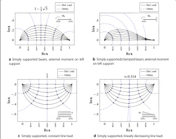
For the present load case, i.e. a simply supported beam, subjected to an external moment at the left node (see also Fig.4), we have
N1,2,0= −3(1−ξ)4+4(1−ξ)3, (40a)
N1,2,1= −3ξ4+4ξ3. (40b)
Withβ1,2,0=1,β2,2,0= −12, we obtain
˜
Z:=N1,2,0(ξ)Z1,2,0−
1
2N2,2,0(ξ)Z2,2,0=i
3
2ξ2−3ξ+1 −ξ3+32ξ2
0 0
a b
c d
Simply supported beam, external moment on left support
Simply supported/clamped beam, external moment on left support
Simply supported, linearly decreasing line load Simply supported, constant line load
Fig. 4 Linearized deformation (only rotational degrees of freedom): deformed configuration and orbitsx(s) of points on the neutral axis of the beam
This formula also reveals that the deformation can be expressed as a rotation of each point
of the initial configuration, with rotation center and angle depending on the parameterξ.
Thus, the orbits of the material points under the given deformations are located on circles of different radius and location. For32ξ2−3ξ+1=0, i.e.ξ =1−1
3
√
3, the deformation is a pure translation in thezdirection.
g0(ξ) (x0(ξ))
= ⎧ ⎪ ⎪ ⎪ ⎪ ⎪ ⎨ ⎪ ⎪ ⎪ ⎪ ⎪ ⎩
esexp
⎛ ⎝3
2ξ2−3ξ+1
⎛⎝i −ξ3+32ξ2 3 2ξ2−3ξ+1
i 0 0 ⎞ ⎠ ⎞ ⎠ ξ 1
ifξ=1−13√3,
esexp
0 −ξ3+3 2ξ2i
0 0 ξ 1 =
1−13√3 1 + 1 9 √ 3i 0
s ifξ=1−13√3.
(42)
For a beam simply supported at the left side and clamped at the right side, subjected to an external moment at the left support (see Fig.4), we omit the shape functionN2,2,0(see
Table8 in Appendix 1), and obtainN1,2,0 = (1−ξ)2,β1,2,0 = 1,∂sκ(ξ) = 6ξ −4, as predicted by the linear beam theory, and
g0(ξ) (x0(ξ))=esexp
ξ2−2ξ+1
i 0 0 0 ξ 1 =
es(ξ2−2ξ+1)iξ 1
For a simply supported beam subjected to a constant line load (see Fig. 4), we have N1,2,0 = −3(1−ξ)4+4(1−ξ)3,N2,2,0= −3ξ4+4ξ3. Withβ1,2,0 =1,β2,2,0 = −1, we
obtain∂sκ(ξ)=12ξ2−12ξ, also consistent with the linear beam theory.
Finally, for a simply supported beam subjected to a linearly decreasing line load (see Fig.4), we use the same shape functionsN1,2,0= −3(1−ξ)4+4(1−ξ)3,N2,2,0= −3ξ4+
4ξ3. Withβ1,2,0=1,β2,2,0=1, we obtain∂sκ(ξ)= −120ξ3+180ξ2−60ξ, conforming to the results of the linear beam theory.
These cases demonstrate that for some simple load cases, the tangent spaceTu(gξ) of the function space of the LogFE formulation at the origin, i.e. foru=0, contains the deflection functions obtained by the linear beam theory. Naturally, for more complicated load cases, Tu(gξ) will not be large enough to contain the exact linear deflection function. For larger deformations, the linearized logarithmic deformation function, just as the conventional linearized deflection curve, does not adequately represent the actual deformation of the beam.
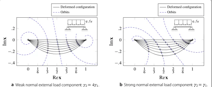
The general case
In the general case, which includes, e.g., the deformation within a single step of a Newton-Raphson approximation, the orbits of the material points of the configuration are not located on circles, but on logarithmic spirals with different points of origin.
Figure5presents an example of the general case. For a diagonally applied constant line
loadf, resulting from a combination of a line load perpendicular to the neutral axis,q,
and a line load parallel to the neutral axis,fN, we useN1,2,0 = −3(1−ξ)4+4(1−ξ)3, N2,2,0 = −3ξ4+4ξ3, as above. We set β1,2,0 = γ2, β2,2,0 = γ2, γ2 ∈ R, such that ∂sκ(ξ)=12γ1ξ2−12γ1ξ, consistent with the linear beam theory. As there is a line load in
the direction of the beam, we must also determine the coefficientsβ1,1,0,β2,1,0, which are
related to the dilatations (r=1). Because the impact of the line force in the longitudinal
direction on the curvature of the beam vanishes foru = 0, we can drop the optional
restriction∂pI,2,0 = 0 (see Table8in Appendix 1). Thus, ¯QI = 0 forI ∈ {1,2}, and the shape functions related to the dilatations, which result in a change in the normal force in the linear beam theory, are given asN1,1,0 = (1−ξ)2,N2,1,0 = ξ2. From the linear
theory, we know that ∂fNε(ξ) = 1
EA(−ξ+ 12). Using Eq. 33a, we see thatβ1,1,0 = 12γ1, β2,1,0= −12γ1,γ1∈R, result in∂sε(ξ)= −γ1ξ+12γ1, conforming to the linear theory.
aWeak normal external load component:γ2=4γ1. bStrong normal external load component:γ2=γ1.