https://doi.org/10.5194/ars-15-69-2017
© Author(s) 2017. This work is distributed under the Creative Commons Attribution 3.0 License.
Sparse representation discretization errors in multi-sensor radar
target motion estimation
Hossein Azodi, Uwe Siart, and Thomas F. Eibert
Chair of High-Frequency Engineering, Department of Electrical and Computer Engineering, Technical University of Munich, 80290 Munich, Germany
Correspondence to:Hossein Azodi ([email protected])
Received: 27 December 2016 – Accepted: 5 August 2017 – Published: 21 September 2017
Abstract.In a multi-sensor radar for the estimation of the tar-gets motion states, more than one module of transmitter and receiver are utilized to estimate the positions and velocities of targets, also known as motion states. By applying the com-pressed sensing (CS) reconstruction algorithms, the surveil-lance space needs to be discretized. The effect of the addi-tive errors due to the discretization are studied in this paper. The errors are considered as an additive noise in the well-known under-determined CS problem. By employing prop-erties of these errors, analytical models for its average and variance are derived. Numerous simulations are carried out to verify the analytical model empirically. Furthermore, the probability density functions of discretization errors are es-timated. The analytical model is useful for the optimization of the performance, the efficiency and the success rate in CS reconstruction for radar as well as many other applications.
1 Introduction
A multi-sensor radar system contains more than one module of transmitter and receiver. These modules are usually posi-tioned separately to increase the spatial diversity, the cover-age or both. A multi-sensor radar system might be config-ured in mono-static, bi-static or multi-static, also known as multiple input mutiple output (MIMO) radar (Skolnik, 1962). The estimation of the positions and velocities of moving tar-gets, also known as motion states, in the surveillance space is a typical use-case of these radars. A more particular ap-plication of these radars is to prevent collisions among ob-jects in the surveillance space by estimating the motion states in relatively short intervals (Azodi et al., 2013, 2015). For the data fusion and the processing, there are various
possi-bilities, especially among the algorithms in the framework of compressed sensing (CS). Compressed sensing is under-stood as a set of information and estimation algorithms for compressible signal processing (Candes et al., 2006; Candès, 2006; Donoho, 2006; Baraniuk, 2007). Despite the Shannon-Nyquist theorem, which asserts a high sampling rate, CS es-timation algorithms reconstruct a signal from far fewer sam-ples. CS algorithms have been applied to multi-sensor radar systems, medical imaging, remote sensing, and many other signal recovery problems in recent years (Duarte and Eldar, 2011).
Sparse representation and finding the solution of the sparse vectorsin the under-determined problem
d=9s (1)
are the primary objectives of CS signal recovery algorithms. In Eq. (1),9 anddare the so-called sensing matrix and the measurement vector, respectively. Basically, Eq. (1) repre-sents an under-determined set of linear equations, where con-tributions of noise and other errors are neglected. In realis-tic data processing, the measured vector is slightly perturbed due to unavoidable measurement system noise and model-ing errors, e.g., due to truncation, roundmodel-ing, or discretization. The perturbation in such cases is often modeled as a Gaussian distributed random signal. Therefore, the problem in Eq. (1) turns into
d=9s+e, (2)
The recovery of the sparse vector from the CS under-determined systems is successful if a number of conditions are met. Since any under-determined problem exhibits an in-finite number of solutions, these conditions are necessary to make sure that the reconstructed solution is the correct one. One of the prevailing conditions is sparsity of the unknown vectors. Other conditions postulate certain properties of the sensing matrix 9 like coherence, restricted isometry prop-erty (RIP), or the null-space propprop-erty (NSP). These condi-tions and their interrelation with the sparsity of s are well elaborated in Foucart and Rauhut (2013), Eldar and Kutyniok (2012) and Donoho (2006).
Recently, CS algorithms have also been utilized for the de-tection of point-like targets in multi-sensor or multiple-input multiple-output (MIMO) radar systems, where a sufficient number of transmitters and receivers observe the surveil-lance space (Eldar et al., 2010; Ender, 2013; Anitori et al., 2013). Typically in these radar systems, number and motion states, initial positions and velocities, of the targets are the unknowns. Compared with conventional methods, CS may achieve identical detection performance with a reduced num-ber of sensors. It may also provide higher resolution and ac-curacy (Donoho and Tanner, 2010; Herman and Strohmer, 2009; Lehmann et al., 2006). Nevertheless, a few additional assumptions are required so that such problems become com-patible with the CS recovery methods. Apart from the already mentioned sparsity of the scene, these are exact phase syn-chronization between transceivers, electromagnetic far-field condition, non-relativistic movements, constant radar cross section (RCS) during one observation and considering tar-gets as point-like scatterers with their motion states at the centers of the grid cells. These assumptions, except the last one, are mostly valid for high-frequency radar systems, par-ticularly for target motion estimation where indeed only few targets exist in the entire vacant surveillance space (Fishler et al., 2006; Haimovich et al., 2008). Also, the approxima-tion of extended targets by an ensemble of point-like scatter-ers is often possible in the high-frequency regime (Hurst and Mittra, 1987).
However, a rather fine grid might be required to warrant the last assumption. Otherwise, it is not justified to assume that the motion states are located at the centers of grid cells. A very fine grid results in a highly coherent sensing matrix which not only causes more computational complexity, but also increases the ambiguity in the reconstruction process. In radar applications, such as collision avoidance radars (Azodi et al., 2014; Wächter et al., 2014), assuming a very fine dis-cretization is not even practical as out-bound targets1 con-siderably enlarge the solution domain. Targets, whose true motion states lie offside the grid points of the discretized so-lution domain, are commonly referred to as off-grid targets
1Assuming a boundary in the scene which encompasses the
radar sensors, the bound targets are those which are located out-side this boundary.
(Tan and Nehorai, 2014; Nielsen et al., 2012; Tang et al., 2012; Gurbuz et al., 2013). It is beneficial to analyze the im-pact of off-grid targets on the CS recovery process and to modify it, accordingly. This impact is studied by analytically modeling it as errors added to the principal CS problem (1) in this work. The main purpose is to find an implicit and pa-rameterized model of these errors. Since such errors are not limited to off-grid targets of radar applications and are seen in various CS problems, the term “discretization error” is used in this work as it reflects the source of errors in a more gen-eral and universal way than off-grid targets effect.
The majority of previous works do not render a rigorous distinction between system noise and discretization errors. Both are summarized in a single Gaussian random signal model at the right-hand side of Eq. (2), although they have different sources and might have different impacts on the problem. This work discriminates between these perturba-tion sources and studies the particular impact of discretiza-tion errors on CS reconstrucdiscretiza-tion algorithms. In this view, the realistic CS problem is represented by
d=9s+es+ed, (3)
wherees anded are system noise and discretization errors, respectively. Also, Eq. (3) implies that, even in a fictitious noise-free system, where measurements are carried out with unlimited accuracy, the discretization errorsedstill remains and cannot be ignored.
The formation of the CS under-determined problem is ex-plained in Sect. 2. An analytical model of the received echo is considered based on geometrical optics. Utilizing the sig-nal model in Sect. 2, the approximated discretization er-rors are calculated in Sect. 3 for two-dimensional geome-tries. The methods and models of this work are not limited to two-dimensional problems and can be extended to three-dimensional configurations. The proposed model is tested by and verified against an extensive number of computer simu-lations. The results of these numerical experiments are gath-ered in Sect. 4. Section 5 finalizes the paper with some con-clusion remarks.
2 Single carrier continuous wave signal model
A typical 2-D scene for target motion estimation using radar sensors is illustrated in Fig. 1. A small number of targets (marked by stars) move in the surveillance area of a Doppler radar system with N mono-static sensors. The wavelength of the transmitted signal as compared to the physical dimen-sions is considered short enough to apply the asymptotic ap-proximations in the calculation of the received signal and to model it analytically.
In a single frequency continuous wave (CW) radar system, each sensor transmits the signal
wherefcandθnare the carrier frequency and initial phase of
the transmitted signal. The received echo from the targets at thenth sensor is
dn(t )= P
X
p=1 apexp
j2π fc(t−τp,n)+θn +es(t ) , (5) wherees(t )is a random signal with zero-mean Gaussian dis-tributionN(0, σ )to represent the system noise. Each coeffi-cientap represents the amplitude of the echo received from
thepth target. These include the system response, free space path loss, and the target’s RCS. Also, τp,n is the effective
round-trip delay between thenth module and thepth target. Having thenth module atrn=rxnxˆ+rynyˆand thepth target
at
rp=(rxp+vxpt )xˆ+(ryp+vypt )y ,ˆ (6)
the round-trip delay is
τp,n=
2
c0
(rxp−rxn+vxpt )2+(ryp−ryn+vypt )2 12
. (7) The carrier exp{j2π fct+θn} in Eq. (5) is removed after
down-conversion and subsequent analog-to-digital conver-sion (ADC). Sampling generates the data series
dn[i] = P
X
p=1
apχp,n[i] +ees[i], (8) whereees(t )is the colored baseband noise and
χp,n[i] =exp
−j4πfc c0
(rxp−rxn+vxpiT )2
+(ryp−ryn+vypiT )2
12
(9) wherec0is the vacuum speed of light andT is the sampling interval.
Let’s assume that every sensor collectsLsamples during one observation. The total number ofN×Lindependent data samples is concatenated in a column vectordaccording to
d=
d1[1], . . ., d1[L], d2[1], . . ., d2[L],
.. . dN[1], . . ., dN[L],
T
(10)
where the superscript T denotes the vector transpose. By maintaining the concatenation order in Eq. (10), Eq. (8) is rewritten in matrix form according to
d=Xa+
ees. (11)
Vectorees embodies the additive noise in each sample. The amplitudes of the echoes are gathered ina= [a1. . .aP]Tand
X=
χ1,1[1] χ2,1[1] . . . χP ,1[1] χ1,1[2] χ2,1[2] . . . χP ,1[2]
..
. ... . . . ... χ1,N[L] χ2,N[L] . . . χP ,N[L]
.
x y
rn r*
Cell center Cell border Mov. target Sensor
vp rp
Figure 1.Targets move in the surrounding space of a multi-sensor radar system. The sensors and the targets are displayed by squares and stars, respectively. The arrows illustrate relative velocities of the targets. The dashed lines are the border of the cells. The centers of the cells are depicted by circles.
Every column ofXrepresents the received samples of a tar-get following the same concatenation order asd. For exam-ple, in explicit notation, thepth column ofXis
χp=
χp,1[1], . . ., χp,1[L], χp,2[1], . . ., χp,2[L],
.. .
χp,N[1], . . ., χp,N[L]
T
. (12)
Equation (11) is not yet in a suitable form, since the un-knowns appear in bothX anda. Furthermore, the size of
ais unknown as usually in a radar problem a priori knowl-edge about the number of targets is not available. Hence, a systematic solution algorithm cannot be proposed yet.
This is, where the CS methodology comes into play. It transforms Eq. (11) into a solvable set of equations in the form
d=Zs+e. (13)
Each column ofZcorresponds to one element from the dis-cretized solution domainSd. The solution domain is a set of all considered target positions together with all permissible velocities, also referred to as states. The matrixZhas, there-fore, an extremely large number of columns as it includes one column for each possible state. The vectorsis the unknown solution vector of Eq. (13). It maps the matrixZto the prob-lem in Eq. (11), i.e., the non-zero eprob-lements ofs correspond to the occupied states found in the measured data.
If, in Eq. (12), one perceives χp as a function of rxp, ryp, vxpandvypin the formχp=χ(rxp, ryp, vxp, vyp),
then theqth column ofZis
ζq=χ(rxq, ryq, vxq, vyq) (14)
whererxq, ryq, vxqandvyqare just theqth state tuple.
This a priori knowledge is relevant for arranging and solv-ing Eq. (13). Short range radars and radar networks with in-bound targets can be cited as exemplary applications. In fact, the search for motion states within an unlimited vari-ety may become highly ambiguous. With limited ranges the discretized solution domain is a set of the form
Sd= {(rxq, ryq, vxq, vyq)| −R≤rxq, ryq≤R,
−V ≤vxq, vyq≤V , q=1,2, . . ., Q}. (15)
Notice that the elements of the solution domain belong toR4
since they cover 2-D locations together with 2-D velocities. With a sufficiently fine discretization of the solution domain, the motion states of the targets are estimated by
sq=
(
ap ifpth target is atqth bin,
0 otherwise. (16)
For the rest of this work, it is assumed that ap is equal to
one for all targets and radar constellations. If only P tar-gets exist in the scene,sis aP-sparse vector with the non-zeros corresponding to the amplitudes of the existing targets. Thus, Eq. (13) represents a CS problem based on the assump-tion thatP QandN L < Q. The vectorsmaps the sensing matrixZto the measured data. By definition, it is zero every-where except for the corresponding elements due to the exist-ing targets. Therefore, the termZsin Eq. (13) is the weighted summation of the selectedP columns ofZcorresponding to the non-zeros ofs.
In Eq. (13),erepresents both, system noise and discretiza-tion errors. For the rest of this work, the system noise is ig-nored. Discretization errors as the remaining part of e are introduced and studied in the next section. System noise may be added to the proposed model as a Gaussian distributed random variable for any future analysis.
3 Discretization errors model
As the target states may lay aside from the centers of the grid cells, the received signal d is not necessarily equal to the summation of the corresponding P columns inZ. As a result, the CS reconstructed signal of a successful recovery is not exactly equal to the measured echoes. This inevitable difference exists even though the discretization is very fine. The characterization of this error plays an important role for the implementation of an efficient and robust recovery algo-rithm. As the error is the result of modeling, improving sys-tem parameters such as the antenna or the amplifier gains do not help to suppress it. An extremely fine mesh may re-duce the discretization errors but only at the cost of a more complex recovery process. Therefore, the better solution is to specifically characterize this error and to modify the recovery algorithm accordingly.
For the characterization of discretization errors, it is as-sumed that the vector d is measured with unlimited accu-racy and the corresponding solution of the CS problem, i.e.,
the optimum solution, is known. The discretization errors are the difference between the optimum solutionsoptand the re-ceived signal as
ed=d−Zsopt. (17)
At this point, it is also assumed that there is only one tar-get present in the scene. As Eq. (17) is linear and existence, positions and velocities of the targets are independent, the discretization errors of more than one target are simply the summation of the discretization errors as in
ed=
P
X
p=1
edp, (18)
where edp is the discretization errors due to the pth
tar-get. It is expected that the optimum solution sopt corre-sponds to the closest(rxopt, r
opt
y , v
opt
x , v
opt
y )in the discretized
solution domain to the target true position and velocity (rxtar, rytar, vxtar, vytar), which means
rtar=ropt+1r
=(rxopt+vxoptt+u11rx/2+u31vxt /2)xˆ
+(ryopt+v
optt
y u21ry/2+u41vyt /2)yˆ (19)
where1rx, 1ry,1vx and 1vy are discretization steps in
rx,ry,vx andvy, respectively, andum fori=1,2,3,4 are
random variables with uniform distributions fUm(um)=
(
1/2 −1≤um≤1
0 otherwise, (20)
because every position and every velocity are assumed equally likely. As no preference for the position of the sen-sors is considered, the characteristics of the discretization er-rors such as expected value or variance becomes indepen-dent of the sensors. It is, therefore, sufficient to study the discretization errors in a one-sensor scene. Under these cir-cumstances, the discretization errors term turns into
ed[i] =exp−j2π fcτtar −exp−j2π fcτopt . (21) Assuming1τ=τtar−τoptis the difference between the true round-trip time of the target and its estimate,ed[i]is approx-imated as
ed[i] = −j2π fc1τexp−j2π fcτopt +O(1τ2) (22) based on the Taylor expansion up to the first order and that 1ττtar. Using a Taylor expansion to approximate1r, it is found that,
|ropt+1r−rsen| = |ropt−rsen| +(r
opt−rsen)·1r
|ropt−rsen|
+O(|1r|2) , (23)
wherersen indicates the position of the sensor in the scene. Hence,
1τ≈2
c
(ropt−rsen)·1r
Using the approximated differences,ed[i]becomes
ed≈ −j4π fc c0
(ropt−rsen)·1r |ropt−rsen|
exp
−j4π fc c0
|ropt−rsen|
. (25)
This linear approximation is accurate as long as the dis-cretization steps in both, space and velocity, are small enough. However, in a typical Doppler-only configuration, the size of the discretization steps in position can be even larger than the wavelength. In these configurations, the ini-tial phase error due to the position have to be removed so that only the error due to the discretization of the velocity remains.
3.1 Expected value of discretization errors
The expected value E{ed}of the discretization errors is an important measure to study this random variable. By defini-tion,
E{ed} = 1
Q Q
X
q=1
Z Z Z
∞
Z
−∞
edqfU1,...,U4(u1, . . ., u4)du1. . .du4 (26)
where q=1,2, . . ., Qruns over the grid of the discretized solution domain and
edq≈ −j2π fc1τqexp−j2π fcτq (27)
is the discretization errors at theqth cell. If theums are
sta-tistically independent, the joint probability density function (PDF) is
fU1,...,U4(u1, . . ., u4)=fU1(u1). . .fU4(u4)
= (
1/16, −1 [u1, . . ., u4]T1
0, otherwise (28)
where the symbol means component-wise less than or equal. Combining Eqs. (22) and (28) with Eq. (26) results in
E{ed} =
−j π fc
8c0QL L X
i=1 Q X
q=1
exp
−j2π fcτq Z Z ZZ1
−1
1τqdu1. . .du4
.
(29) In order to be able to find a feasible solution,1τqis assumed
to be an odd function ofu1,u2,u3andu4, the integration of this function between symmetric boundaries is equal to zero. So, it is derived that
E{ed} =0. (30)
This is an expected result and is also verified with the simu-lations.
3.2 Variance of discretization errors
By definition, the variance of the discretization errors is
V{ed} =E
(ed−E{ed}) (ed−E{ed})∗ , (31) where the asterisk indicates complex conjugates. By insert-ingE{ed}from Eq. (30) into Eq. (31), it becomes
V{ed} =E
ede∗d =4π 2f2
c E{(1τ )2}. (32) Hence,
V{ed} =16π
2f2 c c20QL
L X i=1 Q X q=1 Z Z Z
∞ Z
−∞
(ropt−rsen)·1r
|ropt−rsen| 2
fU1,...,U4(u1, . . ., u4)du1. . .du4. (33)
Having(ropt−rsen)x and(ropt−rsen)y, respectively, thex
andycomponents of(ropt−rsen), Eq. (33) becomes
V{ed} =
4π2fc2
4c2 0QL
L X
i=1 Q X
q=1 Z Z ZZ1
−1
(ropt−rsen)
x(u11rx+u3iT 1vx)+(ropt−rsen)y(u21ry+u4iT 1vy)2
|ropt−rsen|2
×fU1,...,U4(u1, . . ., u4)du1. . .du4. (34)
For the calculation of the variance, it is important to note that 1 Z −1 1 Z −1
uiujduiduj=
(
0 i6=j, 2/3 i=j.
Therefore, the variance in Eq. (35) transforms into
V{ed} =
16π2f2 c
9c02QL
L X
i=1 Q X
q=1
(ropt−rsen)2
x(1r2x+i2T21v2x)+(ropt−rsen)2y(1ry2+i2T21vy2)
|ropt−rsen|2 . (35)
Assuming uniform discretization steps (Fig. 2), i.e., 1rx=1ry=1rxy and 1vx=1vy=1vxy the variance
in Eq. (35) simplifies into
V{ed}=
16π2f2 c
9c20QL L X
i=1
Q X
q=1
(1rxy2 +i2T21vxy2 )
=16π
2f2 c
9c20
1rxy2 +1
6(2L
2+3L+1)T21v2
xy
(36)
x y
R R
x
y
All possible velocities for a single spatial cell.
q v
R R
Figure 2.Discretization inxandy. The discretization in velocity is shown by vectors from the center of the spatial grid cell.
Table 1.Definitions and values of the variables used for empirical assessments.
Variable Value Unit Description
T 4 ms sampling time
fc 24 GHz carrier frequency
xmin −1 m lower bound ofx
xmax 1 m upper bound ofx
ymin −1 m lower bound ofy
ymax 1 m upper bound ofy
vmin −0.25 m s−1 lower bound ofv
vmax 0.25 m s−1 upper bound ofv
Hence, the deviation from the centers of the cells, from which the discretization errors are computed, becomes larger. For a Doppler-only configuration, as of interest in this paper, the size of the grid cells is typically larger than the wavelength and, thus, the initial phase difference due to the position, ac-cording to the term with1rxy2 in Eq. (36), would lead to very larger errors, which are not in agreement with the utilized as-sumption anymore. Therefore, the1rxy2 term is not consid-ered in our later evaluation of the error. In a practical radar application, the initial phase difference can be determined without discretization error, if an appropriate signal process-ing procedure is adopted.
4 Empirical results of discretization errors
Apart from the analytical solution, a possible approach for the characterization of the discretization errors is an empiri-cal study. This can be a substitute method for applications in which finding the analytical solution is not straightforward.
In the empirical method, the difference between the best (or optimum) solution of the compressed sensing and the re-ceived signal is found by executing a large number of random constellations in a Monte Carlo experiment. It is important to
Figure 3.Variance of the discretization errors empirically computed for 5×10⁵targets in every constellation. The amplitudes of the re-ceived signals from the targets are assumed to be one. The variance is normalized to this amplitude and is reported in dB. The number of steps inrxandryand number of steps invxandvyareQr and
Qv, respectively, i.e.,Qrx=Qry=QrandQvx =Qvy =Qv.
¡25 ¡15 ¡5 5 15 25
0 2 4 6 8 10 12 14
(Hz)
)(
H
z
¡
1£
10
¡
2)
= 34
= 6
= 94
= 124
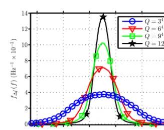
Figure 4.PDF of1fDcomputed for 4 scenarios. In this graph,Q
indicates the total number of grid cells. For example,Q=34means there are 3 steps in each parameter and, hence, in total 81 cells exist.
note that the characterization of the discretization errors is no more a radar problem. Thus, for a given target, it is possible and also required to know the optimum solution as a priori without running any reconstruction algorithm.
Simulations for this purpose are set up based on the data of Table 1. Then, a target with an arbitrarily chosen initial state, i.e., position and velocity, is considered in the scene. The initial state is in accordance with the solution domain limits. Based on the considered state, there is one cell among all grid cells which describes the state of the target the best. This is the reference cell for finding the discretization errors. This experiment is carried out for a large number of target states so that the discretization errors can be studied statisti-cally.
not considered in the simulation results. As expected, the re-sults show that the discretization errors will be reduced by decreasing the discretization steps.
The discretization of the velocity leads to a difference be-tween target’s true Doppler and its estimation, considered as 1fD=fDtar−f
opt
D , in which fDtar and f opt
D are the target’s true Doppler and the estimated Doppler, respectively. Having the same configuration as above, in a further experiment, the PDF of1fDis estimated for 4 scenarios (Fig. 4). These sce-narios vary with respect to the number of steps chosen to dis-cretize the parameters. For each scenario, 5 sensors are used to find the difference between the Doppler frequency created by the 7.5×10⁵targets in the scene and the estimated ones. As shown in this figure, the average is very close to zero, which verifies the derivation in Eq. (30). The variance is also decreasing by increasing the number of discretization steps.
5 Conclusion
The discretization errors have been studied in this work as a separate source of impairments in an ideal Compressed Sens-ing problem. These errors, which occur due to discretization of the solution domain, are a result of modeling and can-not be suppressed by improving system attributes such as the input power or the system gain. Also, in a noise-less sys-tem, where measurements are carried out with infinite pre-cision, these errors are still existing. The study showed that recovery without considering these errors leads to false or improper results. Including discretization errors helps to re-duce the number of the iterations as well as the complexity of the recovery process. The recovery robustness increases by including these errors. The error was characterized analyti-cally by taking the difference between the optimum solution derived by compressed sensing reconstruction algorithm and uniformly distributed targets in the solution domain. Further-more, empirical results of the discretization errors obtained from a large number of simulations have been presented.
Data availability. The underlying research data can be requested from the authors.
Competing interests. The authors declare that they have no conflict of interest.
This work was supported by the German Research Foundation (DFG) and the Technische Universität München within the funding programme Open Access Publishing.
Edited by: Jens Anders
Reviewed by: two anonymous referees
References
Anitori, L., Maleki, A., Otten, M., Baraniuk, R., and Hoogeboom, P.: Design and Analysis of Compressed Sensing Radar Detectors, IEEE T. Signal Proces., 61, 813–827, 2013.
Azodi, H., Siart, U., and Eibert, T.: A Fast Three-Dimensional De-terministic Ray Tracing Coverage Simulator for a 24 GHz Anti-Collision Radar, Adv. Radio Sci., 11, 55–60, 2013.
Azodi, H., Wächter, T., Siart, U., Eibert, T., and Bonerz, S.: Com-pressed Sensing Approach for Fast Collision Warning Radar, in: Proceedings of German Microwave Conference (GeMiC), Aachen, Germany, 2014.
Azodi, H., Siart, U., and Eibert, T.: A Fast 3-D Deterministic Ray Tracing Coverage Simulator Including Creeping Rays Based On Geometry Voxelization Technique, IEEE T. Antenn. Propag., 63, 210–220, 2015.
Baraniuk, R.: Compressive Sensing [Lecture Notes], IEEE Signal Processing Magagazine, 24, 118–121, 2007.
Candès, E.: Compressive Sampling, Proceedings of the Interna-tional Congress of Mathematicians, 1433–1452, Madrid, Spain, 2006.
Candes, E., Romberg, J., and Tao, T.: Stable Signal Recovery From Incomplete and Inaccurate Measurements, Commun. Pur. Appl. Math., 59, 1207–1223, 2006.
Chen, S., Donoho, D., and Saunders, M.: Atomic Decomposition by Basis Pursuit, SIAM review, 43, 129–159, 2001.
Donoho, D.: Compressed Sensing, IEEE T. Inform. Theory, 52, 1289–1306, 2006.
Donoho, D. and Tanner, J.: Precise Undersampling Theorems, Pro-ceedings of IEEE, 98, 913–924, 2010.
Duarte, M. and Eldar, Y.: Structured Compressed Sensing: From Theory to Applications, IEEE T. Signal Proces., 59, 4053–4085, 2011.
Eldar, Y. and Kutyniok, G.: Compressed Sensing: Theory and Ap-plications, Cambridge University Press, Cambridge, UK, 2012. Eldar, Y., Kuppinger, P., and Bolcskei, H.: Block-Sparse Signals:
Uncertainty Relations and Efficient Recovery, IEEE T. Signal Proces., 58, 3042–3054, 2010.
Ender, J.: A Brief Review of Compressive Sensing Applied to Radar, in: Proceedings of 14th International Radar Symposium (IRS), Vol. 1, 3–22, Dresden, Germany, 2013.
Fishler, E., Haimovich, A., Blum, R., Cimini Jr, L., Chizhik, D., and Valenzuela, R.: Spatial Diversity in Radars-Models and De-tection Performance, IEEE T. Signal Proces., 54, 823–838, 2006. Foucart, S. and Rauhut, H.: A Mathematical Introduction to
Com-pressive Sensing, Birkhäuser, Basel, Switzerland, 2013. Gurbuz, A., Teke, O., and Arikan, O.: Sparse Ground-Penetrating
Haimovich, A., Blum, R., and Cimini, L.: MIMO Radar With Widely Separated Antennas, IEEE Signal Processing Magazine, 25, 116–129, 2008.
Herman, M. and Strohmer, T.: High-Resolution Radar Via Com-pressed Sensing, IEEE T. Signal Proces., 57, 2275–2284, 2009. Hurst, M. and Mittra, R.: Scattering Center Analysis Via Prony’s
Method, IEEE T. Antenn. Propag., 35, 986–988, 1987.
Lehmann, N., Haimovich, A., Blum, R., and Cimini, L.: High Res-olution Capabilities of MIMO Radar, in: Proceedings of 40th Asilomar Conference on Signals, Systems and Computers (AC-SSC), 25–30, IEEE, 2006.
Nielsen, J. K., Christensen, M. G., and Jensen, S. H.: On com-pressed sensing and the estimation of continuous parameters from noisy observations, in proceedings of 2012 IEEE Interna-tional Conference on Acoustics, Speech and Signal Processing (ICASSP), 3609–3612, Kyoto, IEEE, 2012.
Skolnik, M.: Introduction to Radar Systems, McGraw-Hill, New York City, NY, USA, 1962.
Tan, Z. and Nehorai, A.: Sparse Direction of Arrival Estimation Us-ing Co-Prime Arrays With Off-Grid Targets, IEEE T. Signal Pro-ces., 21, 26–29, 2014.
Tang, G., Bhaskar, B., Shah, P., and Recht, B.: Compressive Sens-ing Off the Grid, in: ProceedSens-ings of 50th Annual Allerton Con-ference on Communication, Control and Computing, 778–785, Monticello, IL, USA, 2012.