The Thirty-Third AAAI Conference on Artificial Intelligence (AAAI-19)
Deep Bayesian Optimization on Attributed Graphs
Jiaxu Cui,
1,2Bo Yang,
1,2∗Xia Hu
31College of Computer Science and Technology, Jilin University, Changchun, China
2Key Laboratory of Symbolic Computation and Knowledge Engineering of Ministry of Education, China 3Department of Computer Science and Engineering, Texas A&M University, College Station, United States
Abstract
Attributed graphs, which contain rich contextual features be-yond just network structure, are ubiquitous and have been observed to benefit various network analytics applications. Graph structure optimization, aiming to find the optimal graphs in terms of some specific measures, has become an effective computational tool in complex network analysis. However, traditional model-free methods suffer from the ex-pensive computational cost of evaluating graphs; existing vectorial Bayesian optimization methods cannot be directly applied to attributed graphs and have the scalability issue due to the use of Gaussian processes (GPs). To bridge the gap, in this paper, we propose a novel scalable Deep Graph Bayesian Optimization (DGBO) method on attributed graphs. The pro-posed DGBO prevents the cubical complexity of the GPs by adopting a deep graph neural network to surrogate black-box functions, and can scale linearly with the number of observa-tions. Intensive experiments are conducted on both artificial and real-world problems, including molecular discovery and urban road network design, and demonstrate the effectiveness of the DGBO compared with the state-of-the-art.
1 Introduction
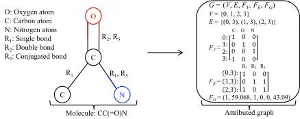
Graphs have been intensively used to model network data generated in important application domains such as chem-istry, transportation, social networks, and knowledge graphs. These real-world networks are often associated with a rich set of available attributes with respect to nodes, edges, and global structures, which are known as attributed graphs. Fig.1 provides one example, in which atomic type, chemical bond type, molecular weight, polar surface area, and other attributes are observed on each molecule. It has been studied that the attributes on graphs are highly correlated to topolog-ical structures (Zhang, Ding, and Milojevi´c 2013) and can benefit various network analysis tasks such as trust predic-tion (Tang et al. 2013) and network embedding (Huang, Li, and Hu 2017). Motivated by these observations, in this work we propose to study whether the attributes on graphs can benefit the task of graph structure optimization and how to comprehensively explore available attributes to address this task more efficiently and effectively.
∗Corresponding author. [email protected]
Copyright c2019, Association for the Advancement of Artificial Intelligence (www.aaai.org). All rights reserved.
Attributed graph G =(V, E, FV, FE, FG)
V= {0, 1, 2, 3}
E = {(0, 3), (1, 3), (2, 3)} C O N
FV =
0: 1: 2: 3: 1 0 01 00 0 0 1 1 0 0
R1R2R3 FE=
(0,3): 1,3 : 2,3 :
1 0 0 0 1 1 1 0 1 FG = (1, 59.068, 1, 0, 0, 43.09)
O: Oxygen atom C: Carbon atom N: Nitrogen atom R1: Single bond
R2: Double bond
R3: Conjugated bond
Molecule: CC(=O)N
O
C
C N
R1 R1, R3
R2, R3
Figure 1: An illustration from a molecule sampling in De-laney data set (DeDe-laney 2004) to an attributed graph (defined in Section 2). Node feature is atomic type, edge feature is chemical bond type, and global attributes contain minimum degree, molecular weight, # h-bond donors, # rings, # rotat-able bonds, and polar surface area.
Optimizing the graph structure is a fundamental task in network analysis, aiming to find the optimal graphs with re-spect to some specific measures. Examples include discover-ing molecular structures with desired properties and design-ing road networks with better traffic conditions. In the lit-erature, existing graph structure optimization methods gen-erally fall into two categories, i.e., model-free methods and model-based methods.
The model-free methods based on evolutionary strategies or annealing strategies have been widely applied to road network design (Xiong and Schneider 1992; Miandoabchi and Farahani 2010; Farahani et al. 2013) and molecular dis-covery (Supady, Blum, and Baldauf 2015; Rupakheti et al. 2015). However, model-free methods will be less effective if the computational cost of evaluating graphs is expensive, be-cause such methods usually require a large number of evalu-ations to maintain population diversity in finding an optimal solution. This is not acceptable particularly for the tasks with large-scale search spaces. For instance, to evaluate the ef-fectiveness of a candidate molecular structure, one has to do lots of computer-aided simulations involving massive com-puting resources or do actual chemical experiments many times with high costs and potential risks.
that are derivative-free, noisy, and expensive to evaluate with respect to different kinds of resources such as time and en-ergy. Note that, for many graph structure optimization tasks, the objective functions are also black-box. In other words, we do not exactly know the mapping mechanism from struc-tural space to measure space, which determines how the structure of a network will affect its functions or dynamics.
Unfortunately, existing BO algorithms focus on optimiz-ing the objectives with vectorial inputs, such as hyper-parameter optimization (Snoek, Larochelle, and Adams 2012) and robot control (Cully et al. 2015). These meth-ods cannot be directly applied to graphs or particularly at-tributed graphs mainly because 1) graph search space is non-Euclidean, discrete, and usually huge (Polishchuk, Madzhi-dov, and Varnek 2013), and 2) it is difficult for existing BO methods to properly and automatically extract the task-specific features from attributed graphs.
Some efforts have been devoted to employing BO, im-plicitly or exim-plicitly, in optimizing graph structures. For ex-amples, some work (Dalibard, Schaarschmidt, and Yoneki 2017; Gardner et al. 2017) have been proposed to handle simple structures, not arbitrary, of vectorial components, which describe the predefined restrictions among them. Some others (Kandasamy et al. 2018; Ramachandram et al. 2018; Jin, Song, and Hu 2018) were proposed to search op-timal neural network architectures, by defining novel graph kernels to measure the similarities among neural networks. Note that these algorithms are exclusively designed for the task of neural architecture search and cannot be easily ex-tended and applied to other domains.
Very recently, a BO framework was proposed explicitly for graph structure optimization (Cui and Yang 2018), re-ferred to as GBO (graph BO). In GBO, both structure and global attributes of the graph are considered to promote op-timization performance by subtly combining deep graph ker-nels with vectorial kerker-nels. According to their reports, GBO outperforms model-free methods and the BO methods with only graph kernels. Note GBO cannot be naturally extended to attributed graphs, where, except global attributes, the at-tributes of nodes and edges should also be considered.
More importantly, the aforementioned BO methods are mainly based on GPs (Gaussian processes). Although GPs is a very flexible non-parametric model for surrogating un-known functions and can effectively model uncertainty as well, the problem is the time cost of GPs inference grows cu-bically with the number of observations, as it necessitates the inversion of a dense covariance matrix. When search space becomes huge, a larger number of evaluations are needed to find optimal solutions, and thus GPs-based BO will be in-feasible due to its cubic scaling.
To address the above challenges, in this paper, we study the problem of efficiently finding optimal attributed graphs. Specifically, we aim at answering two key questions: 1) How to properly represent attributed graphs and make full use of all available features to assist optimization process? and 2) How to make the optimization process more efficient and scalable? By investigating these questions, we propose a novel global Deep Graph Bayesian Optimization (DGBO) framework on attributed graphs. The key idea is to use a
novel deep graph neural network to surrogate black-box functions instead of GPs. The main contributions of this work are summarized as follows.
• Our proposed DGBO can make full use of available fea-tures to benefit graph structure optimization, and scales linearly with the number of observations.
• The efficacy of the DGBO has been strictly validated on both artificial and real-world problems, which shows it effectively and efficiently handles large-scale problems.
2 Problem Statement
The graph structure optimization we studied in this paper is described as: given a graph search space G and a task-specific expensive-to-evaluate black-box functionf : G →
R, we aim at finding the optimal graphG∗ ∈ G with the
maximum value off at as low cost as possible.
Mathemati-cally, this problem is defined as:
G∗= arg max
G∈G
[f(G) +], (1)
whereis the noise of evaluations,Gdenotes an attributed
graph defined as follows (see Fig.1 for an example).
Definition 1.(Attributed graph).G = (V, E, FV, FE, FG)
represents an attributed graph, whereV is a set of vertices, E ⊆(V ×V)is a set of edges,DV andDErepresent the
dimension of node features and the number of edge types, respectively, andFV is a |V| ×DV matrix of the features
of all nodes,FEis a|E| ×DE matrix of the features of all
edges,FGis theDG-dimension global attributes of graph.
3 Deep Graph Bayesian Optimization
3.1 The DGBO Framework
To tackle the two challenges mentioned in Section 1, we propose the DGBO framework based on BO. The DGBO poses the graph structure optimization as a sequential deci-sion problem: which graph should be evaluated next so as to maximize the black-boxf as quickly as possible, by taking
into account the information gain with uncertainty obtained from previous evaluations. There are two key components needed to be specified in the DGBO, i.e., a surrogate func-tion and an acquisifunc-tion funcfunc-tion.
integrate a layer of BLR (Bayesian linear regressor) into the proposed deep graph neural network. It is worth noting that it is the introduction of BLR that makes the DGBO achieve linear complexity w.r.t the number of observations. The pro-posed surrogate model will be elaborated in the next section. Acquisition function quantifies the potential of candidate graphs based on previous validations. Given a graph search spaceGand a hyper-parameter spaceΘ, acquisition function
is defined asU : G ×Θ→ R. The EI (expected
improve-ment) (Moˇckus, Tiesis, and Zilinskas 1978) is a commonly used criterion. Letθ be hyper-parameters of the surrogate,
the EI expressesU(G|Dt,θ) = (µ(G)−ymax)Φ(z(G)) +
σ(G)φ(z(G)),wherez(G) = µ(G)−ymax
σ(G) ,µ(G)andσ(G)
are predictive mean and standard deviation (see Eq. 8 and Eq. 9 for details), ymax is the maximum value among current validationsDt ={(G1, y1),(G2, y2), ...,(Gt, yt)},
Φ(.) andφ(.) denote the cumulative distribution function
and probability density function of normal distribution, re-spectively. Herein, we use the MCMC version of EI as described in (Snoek, Larochelle, and Adams 2012). For a fully-Bayesian treatment, this version integrates out hyper-parameters in the posterior distribution of observations, in-stead of point estimation which often causes local optimum. Thus, the final acquisition function is formulated as:
α(G|Dt) = Z
U(G|Dt,θ)dθ∝ S X
i=1
U(G|Dt,θ(i)), (2)
whereθ(i)
∼p(θ|Dt)andp(θ|Dt)is the posterior distribu-tion ofθ, which will be discussed in Section 3.3.
By maximizing the above acquisition function, we can se-lect a potential graph to evaluate next. Then, one can recal-culate the predictive mean and variance of surrogate based on previous validations and reselect next graph to be evalu-ated, until reaching a predefined termination condition. The framework of DGBO is given in Algorithm 1.
3.2 The Proposed Deep Surrogate Model
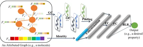
Fig.2 shows the architecture of the proposed surrogate model. Each layer of the surrogate is discussed as follows.
GC
Output (e.g., a desired
property) Fv
FG
Fe
An Attirbuted Graph (e.g., a molecule) Fe
Fe Fe
Fe Fv
Fv Fv
Fv
…
GC Pooling
BLR
Identity
…FC FC
Figure 2: The overview architecture of the surrogate model in the DGBO. Its input is an attributed graph (e.g., a molecu-lar graph) and output is a continuous measure (e.g., a desired property).Fvdenotes the features of nodev,Fedenotes the features of edgeeandFGdenotes global attributes.
Graph convolution (GC) layer. To handle attributed graphs, we use graph convolution technique to automatically extract features of graphs without human intervention.
Algorithm 1:DGBO
Input:Graph search spaceG; The architecture of deep surrogate modelN et; # initialization
evaluationsM; Maximum # iterations M axIter; # hyper-parameter samplingS; # iterations of retrainingRe;
Output:The optimal graphG∗.
1 InitializeM graphs randomly, evaluate them, and
integrate into
D0={(G1, y1),(G2, y2), ...,(GM, yM)};
2 TrainN etwith training setD0;
3 SamplingShyper-parameter samples from their
posterior distributionp(θ|D0);
4 fort= 1,2, ..., M axIterdo
5 Select a potential graphGnextfromGby maximizing Eq.2 using random sampling;
6 Evaluate the black-box system to obtainynext, and
augment dataDt=Dt−1∪ {(Gnext, ynext)};
7 ift%Re== 0then
8 RetrainN etwithDt;
9 ResamplingShyper-parameter samples from the posterior distributionp(θ|Dt);
10 returnG∗with the maximumyinDt.
The existing works related to GC fall into three categories: spatial, spectral, and spectrum-free. Since the surrogate of DGBO is used to approximate a graph regression function, we focus on designing a spectrum-free method, which ac-tually is a polynomial approximation of spectral method. Specifically, we propose a new spectrum-free convolution operation on attributed graphs, which is formulated as:
H(l+1)=σ(
DE
X
r=1
˜
D−1r /2A˜rD˜−1r /2H
(l)
Wr(l+1)), (3)
whereH(l)denotes the hidden representation of all nodes on
layerl,Wr(l+1)denotes the weights on the typer(of edges) at layerl+1, andσ(.)denotes an activation function, such as
ReLU(.) =max(0, .)ortanHfunction.D˜−1/2
r A˜rD˜−1/
2
r denotes the normalization representation of adjacent matrix
Ar, whereA˜r =Ar+I,D˜r =Dr+I,Dris a diagonal
matrix and its diagonal elements are the degree of the corre-sponding nodes on typer. This normalization trick has been
proved to be a first-order approximation of localized spec-tral filters on graphs. Note that, unlike (Schlichtkrull et al. 2017), we utilize this trick instead ofD−1
parameters without the need to calculate eigen-system.
Pooling layer.Through pooling layer, we wish to reason-ably learn the global representation of the whole graph from the local representations of nodes and edges. Accordingly, we propose the following pooling operation:
H(pool)=σ(sumrow(sof tmax(H(l)W(pool)))), (4) whereH(pool)denotes the representation of graph-level
fea-tures,H(l) denotes the output after going through l graph
convolution layers, and W(pool) denotes the weights on
pooling layer. We first multiply H(l) by W(pool) to map
the features obtained by graph convolution into a new latent space with a specified dimension, and then apply
sof tmax(.)to the result to obtain row-wise sparse
repre-sentations and map them into a unified interval[0,1]. Note that the usage ofsof tmax(.)can also prevent ignoring
im-portant rows but having some relatively small-value dimen-sions. Then we apply sumrow(.) to accumulate multiple row-wise features into one vector before applying a nonlin-ear functionσ(.)to obtain final graph-level representation.
Prior layer.The prior knowledge about a graph (such as the weight of a molecule) can be regarded as the global at-tributes of the graph. In addition to prior knowledge, the global information (such as the scale of a graph) or the high-order structural information (such as betweenness centrality or clustering coefficient) that are easy to get can also be re-garded as the global attributes of a graph. All of the available information could potentially promote the performance of optimization. Through the prior layer, such global attributes are expected to be logically integrated into final graph rep-resentation. There might be different ways to do this. In this work, we adopt a simple concatenating strategy in order to make optimization as scalable as possible,
H(con)=Concat(H(pool), λF
G), (5)
whereFGdenotes the global attributes of graph,H(pool) de-notes the representation output by pooling layer, andλis a
switch weight. If global attributes are available, we turnλ
on. Otherwise, we turn it off.
Bayesian linear regressor (BLR) layer.To predict the measure of a graph while capturing uncertainty, we add a Bayesian linear regressor (BLR) just behind multiple FC (fully connected) layers as the last layer of the surrogate architecture. We regard this model as an adaptive basis re-gression and the basis functions are parameterized by the weights and biases of the deep neural network. BLR is for-mulated as:
y1:N = Φ(.)Tw+b, (6)
wherey1:N denotes outputs,b ∼ N(0, σ2noiseI),N(.)is normal distribution,σ2
noiseis noise level, wis the weights of BLR layer, andΦ(.)is the decision matrix output by
pre-vious layers as the input of BLR layer. Given a prior distri-bution on weights:w ∼ N(0, σ2
wI), whereσw2 denotes the
uncertainty ofw, the measure ofG∗can be predicted by: y∗|D1:N,y1:N, G∗∼ N(µ(G∗), σ2(G∗)), (7) whereD1:N are observations,y1:N are evaluated measures,
µ(G∗) =σ−2noiseΦ(G∗)TK−1Φ(.)y1:N, (8)
σ2(G∗) = Φ(G∗)TK−1Φ(G∗) +σ2
noise. (9)
K = σnoise−2 Φ(.)Φ(.)T +σ−2
w I. Note that this layer is the
key to reduce time complexity (see Section 3.4 for details).
Loss function. Having each layer of the deep surrogate model, we use the following loss function to train it,loss=
PN
i=1|yˆi−yi| 2+γ
||Ω||2l
2,whereyˆidenotes predictive
out-put,yidenotes ground truth,Ωdenotes the weights and bi-ases of neural network, andγdenotes penalty coefficient.
3.3 Implementation Details
Handling hyper-parameters.In the proposed deep surro-gate model, all hyper-parameters need to handle includeΩ in loss function (the weights and biases of GC, pooling and FC layers) andθin Eq. 2 (σ2
wandσnoise2 of BLR layer). For Ω, we train GC, pooling and FC layers via backpropagation and a wildly used stochastic gradient descent named Adam (Kingma and Ba 2015). In this training phase, we use a linear output layer to replace BLR. This process can be viewed as a MAP estimate of all parameters in these layers. Based on the parameterized basis functions, we make predictions by a BLR. Thereby we need to deal withθof the BLR layer. For a
full-Bayesian treatment, we integrate outθ ={σ2
w, σ2noise} by using an ensemble MCMC sampler (Foreman-Mackey et al. 2013), according to their posterior distributionp(θ|D). For the posterior distribution, we place a logarithmic normal prior with mean -10 and standard deviation 0.1 onσ−2
w , and
a horseshoe prior with scale 0.1 onσ2
noise. Then, the poste-rior is obtained byp(θ|D)∝p(D|θ)p(θ), wherep(D|θ)is the marginal likelihood of evaluations.
Basis regularization.Note that, in Eq. 3, the number of parametersW1, W2, ..., WDE will increase rapidly with the
number of edge types DE on each GC layer. Hence we adopt basis regularizationto prevent overfitting by
reduc-ing the number of parameters. Basis regularization assumes that different relations may partially share common param-eters. Specifically, we assume thatWr(l+1)consists of a lin-ear combination of bases{V1(l+1), V
(l+1) 2 , ..., V
(l+1)
B }, i.e.,
Wr(l+1)=PBb=1β (l+1)
r,b V
(l+1)
b , whereβis combination co-efficient andBis the number of bases.
and 500 for testing. Then, we use a GPs-based BO to op-timize architecture based on CEP. The optimal architecture obtained in this way is shown in Table 1. We will apply the architecture to all tasks discussed in our experiments.
Parameters Ranges Optimal
# GC layers {1, 2, 3, 4, 5} 5
# FC layers {1, 2, 3, 4, 5} 5
# units of GC [10, 100] 48
# units of pooling [10, 100] 50
# units of FC [10, 100] 45
σ(.)of GC {ReLU,tanH} tanH σ(.)of pooling {Identity,ReLU,tanH} Identity
σ(.)of FC {Identity,ReLU,tanH} tanH
Learning rate [1e-4, 1e-1] 1e-4
Dropout [0, 1] 0.0
Penalty coefficient [1e-5, 1e-1] 1e-5
Table 1: The optimal surrogate architecture.
3.4 Time Complexity Analysis
In BO-style optimization, maximizing acquisition function is often the bottleneck of efficiency. If the surrogate is GPs, it will takeO(N3)time to compute the inverse of anN-by-N
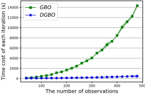
kernel matrix and then, based on it, to predict the mean and variance required by acquisition function.N is the number of validations. Similarly, in the DGBO, maximizing acqui-sition function (step 5 in Algorithm 1) is still the most ex-pensive relative to others (including training deep surrogate in step 8), which dominates the overall time of the DGBO. We will see, by using the proposed deep surrogate, the time for quantifying acquisition function will be greatly reduced to linear order. LetM be the number of units on BLR layer. The matricesΦ(·)andKin Eqs. 8 and 9 areN-by-M and M-by-M, respectively. It takesO(M2N)andO(M3)time
to compute K and its inverse. It then takesO(M2N)and O(M2)time to compute Eq. 8 (mean) and Eq. 9 (variance).
NoteM is a constant much less thanN. So the total time
of prediction isO(M2N) = O(N). Moreover, we
empiri-cally validate this by comparing the DGBO to a GPs-based method (GBO) (Cui and Yang 2018). It can be seen from Fig.3 the DGBO increases linearly with the number of vali-dations, far superior to the cubic growth of the GBO.
4 Experiments
Here, we rigorously evaluate the DGBO by answering three questions. 1) Can the available features from attributed graphs benefit optimization? 2) How effective and efficient is the DGBO compared with the start-of-the-art on real-world problems? 3) Can it be applied to various domains?
4.1 Data Sets
The data sets used in this paper are summarized in Table 2.
Syntheticsis artificially generated via the NetworkX tool (Hagberg, Schult, and Swart 2008), which includes 500 undirected random graphs. Note that both the nodes and edges of graphs in this data set do not have features. For the global attributes, we extract 6 features from each graph: #
Figure 3: Comparison of scalability between the DGBO and a non-scalable method GBO on Synthetics (described in sec-tion 4.1).x-axis andy-axis denote # validations and the time
cost of each iteration, respectively. The time cost of each it-eration includes the time of selecting next graph plus the time of retraining deep surrogate network in the DGBO or learning hyper-parameters of kernels in GBO.
Data sets |G| |V| |E| DV DE DG
Synthetics 500 39.8 141.5 - - 2/4/6 Delaney 1,122 13.3 27.4 68 6 6
ZINC 20,000 23.2 24.9 68 6 6 SiouxFalls 32,768 24 30.5 2 - 5
Table 2: Statistics of data sets.|G|denotes the graph num-bers of search space, |V| denotes the average number of nodes, and|E|denotes the average number of edges.
nodesx1, # edgesx2, average degree centralityx3, average
betweenness centralityx4, average clustering coefficientx5, and a completely unrelated random variablex6.
Delaney is a molecular data set having 1,122 molecules whose aqueous solubility has been measured by (Delaney 2004). Node feature is the atomic type, edge feature is the chemical bond type, and each molecule has six additional global attributes (see Fig.1).
ZINCincludes 20,000 drug-like commercially available molecules extracted at random from the ZINC database (Ir-win et al. 2012). The features of node and edge are the same as Delaney. Since ZINC does not provide global attributes for each molecule, we extract some structure information in-cluding # nodes, # edges, average degree centrality, average betweenness centrality, average closeness centrality, and av-erage clustering coefficient as global attributes.
SiouxFalls. This data set is widely used in transportation studies (Leblanc, Morlok, and Pierskalla 1975). Similar to the previous works, we randomly remove a number of roads from the original network, by assuming these roads have not been built yet. We now want to decide which roads of these removed roads should be constructed in order to min-imize total travel time. For example, if we remove 15 roads, there will be215potential assignments, i.e., our search space
Methods Situation(a)(# Evals=90) Situation(b)(# Evals=100) Situation(c)(# Evals=100) Situation(d)(# Evals=120) Random 2.796±0.004 2.796±0.004 2.796±0.004 2.796±0.004
BOvec 2.863±0.000 2.824±0.002 2.828±0.005 2.851±0.000
BOGlets 2.814±0.005 2.834±0.001 2.834±0.001 2.850±0.000
BOdGlets 2.815±0.002 2.815±0.002 2.815±0.002 2.821±0.001
GBOdGlets 2.863±0.000 2.863±0.000 2.863±0.000 2.849±0.000
DGBOnoRel 2.863±0.000 2.863±0.000 2.863±0.000 2.863±0.000
Table 3: Evaluation of the DGBO versus Random and other non-scalable methods on Synthetics in four situations. # Evals represents the evaluation times. The mean and standard deviation ofyare reported. Bold positions are the optimums.
4.2 Baselines and Setup
The baseline methods compared to the DGBO are catego-rized into three groups as follows.
• Random denotes random selection at each iteration. • BO denotes GPs-based BO method integrating different
kernels indicated by the subscript. The specific kernels include Gaussian ARD kernel (BOvec), graphlets kernel (Shervashidze et al. 2009) (BOGlets), and deep graphlets kernel (Yanardag and Vishwanathan 2015) (BOdGlets). As the Gaussian ARD kernel is a vectorial kernel, we firstly extract the features of graph manually, and then ap-ply it to these pre-extracted hand-crafted features. • GBO denotes the GPs-based BO method by combining
a graph kernel and a vectorial kernel (Cui and Yang 2018). Subscript indicates its integrated graph kernel. The specific kernels include deep graph kernels based on graphlets (GBOdGlets), subtree patterns (GBOdW L) and shortest path (GBOdSP), respectively. Note that the first kernel can deal withunlabelledgraphs while the last two
kernels can only deal withlabelledgraphs.
For the proposed method, DGBOnoRel denotes that it ig-nores edge features (i.e., applies Eq. 3 in which DE ≡ 1 to convolute graph), DGBORel denotes that it considers edge features via Eq. 3 without basis regularization, and DGBORelReg denotes that it not only considers edge fea-tures, but also uses basis regularization. Without specifica-tion, both the number of initializing graphsM and the iter-ations of retrainingRe are set to 20,B is set to 4, and all
algorithms run 5 times to eliminate random effects.
4.3 Artificial Non-Linear Function
We firstly test the efficacy of the DGBO on Synthetics. Note that there are no features on nodes in this data set. In this case, a common way to assign features to nodes is: the nodes of the same graph are assigned the same one-hot rep-resentation, in which the entry of 1 corresponds to the in-dex of the graph. We, then, normalize each global attribute into [0,1] via x˜ = x−xmin
xmax−xmin. We define the target y =
−Hart(˜x1,x2,˜ x3,˜ x4˜ ) as the artificial non-linear function
from a graph to a functional measure, whereHart(.) de-notes the four-dimension Hartmann function that is a com-mon non-linear test function in BO community. We test the DGBO to find a graph with the maximumyfrom Synthetics in four situations: (a) properly usingx1˜ ,x2˜ ,x3˜ , andx4˜ as
global attributes; (b) partially usingx1˜ andx2˜ as global at-tributes; (c) totally usingx1˜ ,x2˜ ,x3˜ ,˜x4,x5˜ andx6˜ as global
attributes; (d) falsely using a non-direct related feature x5˜
and a completely unrelated featurex6˜ as global attributes. In Table 3, no matter how the prior knowledge is changed from the situation (a) to (d), the DGBO outperforms other non-scalable methods. Note that the DGBO outperforms BOGletsand BOdGletssignificantly. That implies the graph convolution used in the DGBO is more suitable for attributed graph feature extraction than the existing graph kernels. Moreover, when the global features pre-extracted by hand are unrelated to the objective in question (i.e., situation (d)), all compared methods fail to find the optimum mainly be-cause these handcrafted features may impose a negative ef-fect on optimization process. To prevent overfitting is an-other reason why a simple concatenation fusion rather than a more complicated one is preferred on the prior layer. Note GBOdW Land GBOdSPare not included as both cannot han-dle the graphs in which all nodes have identical labels.
4.4 Molecular Discovery
Molecular discovery is a meaningful problem. However, the optimization in molecular space is extremely challenging because the search space is usually large, and molecules have a rich set of available features (see an illustration in Fig.1). More importantly, it is very expensive to evaluate a molecule by doing regardless of simulations or real experi-ments. Thus, the DGBO is suitable for this problem. Specif-ically, we apply it to discover optimal molecules from two graph spaces of Delaney and ZINC, respectively.
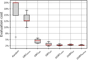
In Delaney, we aim to find a molecule with maximal aque-ous solubility. All methods can find the optimum under a given evaluation budget (i.e., 200), except for Random. In Fig.4, we see that all model-based methods outperform
Ran-Figure 4: Boxplot of evaluation cost for finding the optimum by the DGBO versus other baselines on Delaney.y-axis
dom. GBOdGlets is significantly worse than other model-based methods, as it cannot use node features (i.e., atomic type). Note that our methods outperform others, i.e., they only evaluate about 3% of the whole search space to find the optimum. Meanwhile, they are more robust to initial valida-tions. Moreover, DGBORel and DGBORelReg are slightly more stable than DGBOnoRel, as they take advantage of edge features (i.e., chemical bond type).
To further test the efficacy and scalability of the DGBO on a larger search space, we apply it to ZINC to find an optimal drug-like molecule with maximaly = 5×QED−SAS,
where QED denotes the quantitative estimation of
drug-likeness (Bickerton et al. 2012) andSAS denotes the
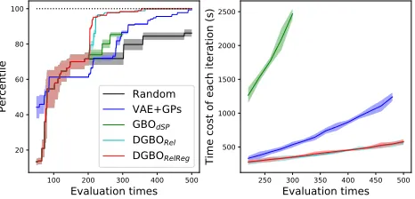
syn-thetic accessibility score (Ertl and Schuffenhauer 2009). That is, we want to find the most drug-like molecule that is also easy to synthesize. In addition, we compare the DGBO with a state-of-the-art technology of automatic chemical de-sign, named as VAE+GPs (G´omez-Bombarelli et al. 2018). The process of the VAE+GPs is as follows: a variational autoencoder (VAE) is firstly trained upon whole ZINC database to map all molecules into a fixed-length (e.g., 196) continuous vector space, and then a GPs-based BO is used to find optimal molecules in this latent space.
100 200 300 400 500
Evaluation times 20 40 60 80 100
Percentile RandomVAE+GPs GBOdSP
DGBORel
DGBORelReg
250 300 350 400 450 500
Evaluation times 500 1000 1500 2000 2500
Time cost of each iteration (s)
Figure 5: Left: Comparison of convergence curves on ZINC.
x-axis represents evaluation times.y-axis represents the per-centile of optimum. We randomly evaluated 200 molecules at the initialization stage and ran all methods on the same hardware setting. Solid lines represent mean values, and shaded regions represent variance. Right: Time cost of each iteration.y-axis represents the time cost of each iteration.
From Fig.5 we see the DGBO outperforms others sig-nificantly and needs the minimal time cost. The DGBO finds the optimum by evaluating only 1.8% of whole search space. DGBORelRegis slightly better than DGBORel, which shows the efficacy of basis regularization. On the other hand, VAE+GPs needs much more evaluations to find a near opti-mum, and its scalability with the number of evaluations is re-markably worse than that of the DGBO. In addition to using expensive GPs, the representation of the graph adopted by it might be another reason for inefficiency. VAE+GPs learns graph representation via an unsupervised manner, which may not be insightful for specific tasks. Note that GBO per-forms poorly because it has to stop much earlier than con-vergence due to its prohibitively high time cost.
4.5 Urban Road Network Design
In order to verify the effectiveness of the DGBO in differ-ent domains, we apply it to address the task of urban road network design (Farahani et al. 2013) on SiouxFalls. Urban road network design is a bi-level optimization problem. The upper-level problem concerns global policy design in prac-tice which aims to achieve an optimal macroscopic measure (e.g., reducing total traveling time) by designing new poli-cies (e.g., where to build new roads). While, the low-level problem cares about how to optimize the behaviors of indi-viduals, e.g., the distribution of traffic flow in a given road net. Herein, we focus on the upper-level road network design problem, and for the lower-level problem, we use the Frank-Wolfe algorithm (Fukushima 1984), a widely used method in transportation, to optimally distribute traffic flows. How-ever, this way usually takes expensive computing resources, particularly for very large road nets. Thus, how to design an optimal road network under a few evaluations is still a chal-lenging problem. In addition, according to (Farahani et al. 2013), genetic algorithm (GA) (Xiong and Schneider 1992) and simulated annealing (SA) (Miandoabchi and Farahani 2010) are two most common optimization algorithms for this problem. Therefore, we compare the DGBO against GA and SA as baselines. Moreover, we use a GPs-based BO to optimize the parameters of GA and SA in order to achieve their best performance (see the right panel of Fig.6).
optimum. Meanwhile, they are more robust to initialize
dif-ferent points. Moreover, DGBOReland DGBORelRegare
slightly more stable than DGBOnoRel, as they take
advan-tage of the edge features (i.e., chemical bond type). To further test the efficacy and scalability of the DGBO on a larger search space, we apply it to ZINC to find an optimal
drug-like molecule with maximaly= 5⇥QED SAS,
whereQEDrepresents the quantitative estimation of
drug-likeness (Bickerton et al. 2012) andSASrepresents the
synthetic accessibility score (Ertl and Schuffenhauer 2009). That is, we want to find the most drug-like molecule that is also easy to synthesize. In addition, we compare the DGBO with a state-of-the-art technology of automatic chemical de-sign, denoted as VAE+GPs (G´omez-Bombarelli et al. 2018). The process of discovering new molecules via VAE+GPs is as follows: a variational autoencoder (VAE) is firstly trained upon the whole ZINC database to map all molecules into a fixed-length (e.g., 196) continuous vector space, and then a GPs-based BO is used to find new molecules in this
latent space. In Fig. 5, we see that both DGBOReland
Figure 5: Left: Comparison of convergence curves on ZINC.
x-axis represents evaluation times.y-axis represents the gap to the optimum. We randomly evaluated 200 molecules at the initialization stage and ran them on the same hardware setting. Solid lines represent the mean values, and shaded regions represent the variance. Right: Time cost of each it-eration.y-axis represents the time cost of each iteration.
DGBORelRegoutperform others significantly and have the
minimal time cost (see the right panel of Fig. 5). The main reason is that the proposed method can make full use of node features, edge features and global attributes. Moreover, DGBORelRegis slightly better than DGBOReland evaluates
only about 6% of whole search space to find the optimum. This shows the efficacy of basis regularization. Note that both GBO and VEA+GPs perform poorly. GBO stops early before its convergence due to its prohibitively high time cost (see the right panel of Fig. 5). The latent space is learned by VEA+GPs via an unsupervised manner. For specific tasks, such a latent representation obtained by unsupervised learn-ing may be less helpful.
4.5 Urban Road Network Design
In order to verify the effectiveness of the DGBO in dif-ferent domains, we apply it to solve the urban road net-work design (Farahani et al. 2013) on SiouxFalls. Urban
road network design is a bi-level optimization problem. The upper-level problem concerns global policy design in prac-tice which aims to achieve an optimal macroscopic measure (e.g., reducing total traveling time) by designing new poli-cies (e.g., where to build new roads). While, the low-level problem cares about how to optimize the behaviors of indi-viduals, e.g., the distribution of traffic flow in a given road net. Herein, we focus on the upper-level road network design problem, and for the lower-level problem, we use the Frank-Wolfe algorithm (Fukushima 1984), a widely used method in transportation, to optimally distribute traffic flows. How-ever, this way usually takes expensive computing resources, particularly for very large road nets. Thus, how to design an optimal road network under a few evaluations is still a chal-lenging problem. In addition, according to (Farahani et al. 2013), genetic algorithm (GA) (Xiong and Schneider 1992) and simulated annealing (SA) (Miandoabchi and Farahani 2010) are two most common optimization algorithms for this problem. Therefore, we compare the DGBO against GA and SA as baselines. Moreover, we use a GPs-based BO to optimize the parameters of GA and SA in order to ensure their best performance (the optimal parameters are shown in the right panel of Fig. 6).
The optimal parameter settings GA Population size is 90
Crossover rate is 0.6 Mutation rate is 0.062 SA # trials per cycle is 2
Initial acceptance probability is 0.7 Final acceptance probability is 0.001
Table 4: The optimal parameters of GA and SA on Sioux-Falls.
optimum. Meanwhile, they are more robust to initialize dif-ferent points. Moreover, DGBOReland DGBORelRegare
slightly more stable than DGBOnoRel, as they take
advan-tage of the edge features (i.e., chemical bond type). To further test the efficacy and scalability of the DGBO on a larger search space, we apply it to ZINC to find an optimal drug-like molecule with maximaly= 5⇥QED SAS, whereQEDrepresents the quantitative estimation of drug-likeness (Bickerton et al. 2012) andSASrepresents the synthetic accessibility score (Ertl and Schuffenhauer 2009). That is, we want to find the most drug-like molecule that is also easy to synthesize. In addition, we compare the DGBO with a state-of-the-art technology of automatic chemical de-sign, denoted as VAE+GPs (G´omez-Bombarelli et al. 2018). The process of discovering new molecules via VAE+GPs is as follows: a variational autoencoder (VAE) is firstly trained upon the whole ZINC database to map all molecules into a fixed-length (e.g., 196) continuous vector space, and then a GPs-based BO is used to find new molecules in this latent space. In Fig. 5, we see that both DGBOReland
Figure 5: Left: Comparison of convergence curves on ZINC.
x-axis represents evaluation times.y-axis represents the gap to the optimum. We randomly evaluated 200 molecules at the initialization stage and ran them on the same hardware setting. Solid lines represent the mean values, and shaded regions represent the variance. Right: Time cost of each it-eration.y-axis represents the time cost of each iteration. DGBORelRegoutperform others significantly and have the
minimal time cost (see right panel of Fig. 5). The main reason is that the proposed method can make full use of node features, edge features and global attributes. Moreover, DGBORelRegis slightly better than DGBOReland evaluates
only about 6% of whole search space to find the optimum. This shows the efficacy of basis regularization. Note that both GBO and VEA+GPs perform poorly. GBO stops early before its convergence due to its prohibitively high time cost (see right panel of Fig. 5). The latent space is learned by VEA+GPs via an unsupervised manner. For specific tasks, such a latent representation obtained by unsupervised learn-ing may be less helpful.
4.5 Urban Road Network Design
In order to verify the effectiveness of the DGBO in dif-ferent domains, we apply it to solve the urban road net-work design (Farahani et al. 2013) on SiouxFalls. Urban
road network design is a bi-level optimization problem. The upper-level problem concerns global policy design in prac-tice which aims to achieve an optimal macroscopic measure (e.g., reducing total traveling time) by designing new poli-cies (e.g., where to build new roads). While, the low-level problem cares about how to optimize the behaviors of indi-viduals, e.g., the distribution of traffic flow in a given road net. Herein, we focus on the upper-level road network design problem, and for the lower-level problem, we use the Frank-Wolfe algorithm (Fukushima 1984), a widely used method in transportation, to optimally distribute traffic flows. How-ever, this way usually takes expensive computing resources, particularly for very large road nets. Thus, how to design an optimal road network under a few evaluations is still a chal-lenging problem. In addition, according to (Farahani et al. 2013), genetic algorithm (GA) (Xiong and Schneider 1992) and simulated annealing (SA) (Miandoabchi and Farahani 2010) are two most common optimization algorithms for this problem. Therefore, we compare the DGBO against GA and SA as baselines. Moreover, we use a GPs-based BO to optimize the parameters of GA and SA in order to ensure their best performance, i.e., population size is 90, crossover rate is 0.6, and mutation rate is 0.062 in the GA, and trials per cycle is 2, initial acceptance probability is 0.7, and final acceptance probability is 0.001 in the SA.
Algorithms The optimal parameter settings GA Population size is 90
Crossover rate is 0.6 Mutation rate is 0.062 SA # trials per cycle is 2 Initial acceptance probability is 0.7 Final acceptance probability is 0.001
Table 4: The optimal parameters of GA and SA on Sioux-Falls.
Figure 6: Convergence comparison of respective methods on urban road network design.y-axis represents the maxi-mal measure value, i.e., the negative logarithm of total travel time.
In Fig. 6, we see that the DGBO outperforms others sig-nificantly. It finds the optimum by no more than 26 evalua-tions (see the embed panel in Fig. 6), which is nearly 3 times faster than the GBO (⇠80 evaluations), and 18 times faster than the GA and SA (⇠450 evaluations). The main reason is that the DGBO can take advantage of both structural features and node features, while the other two cannot. Figure 6: Left: Convergence comparison of respective meth-ods on urban road network design. The left area of the ver-tical dotted line separates the initialization stage. Right: The optimal parameters of the GA and SA.
In Fig. 6, we see that the DGBO outperforms others sig-nificantly. It finds the optimum by no more than 26 evalua-tions (see the left embed panel in Fig. 6), which is nearly 3
times faster than the GBO (⇠80 evaluations), and 18 times
faster than the GA and SA (⇠450 evaluations). The main
reason is that the DGBO can take advantage of both struc-ture and node feastruc-tures, while the other two cannot.
Figure 6: Left: Convergence comparison of respective meth-ods on urban road network design. Right: The optimal pa-rameters of GA and SA.
From Fig.6 we see that the DGBO significantly outper-forms others again. It finds the optimum under less than 420 evaluations, which is nearly 7.7 times faster than the SA (∼3250 evaluations), which runs the second fastest. The main reason is that the DGBO can take advantage of both structure and node features, while the SA and GA cannot. Note GBO stops very early again due to its high time cost.
5 Conclusions
Acknowledgments
This work was supported by the National Natural Sci-ence Foundation of China under grants 61572226 and 61876069, and Jilin Province Key Scientific and Techno-logical Research and Development Project under grants 20180201067GX and 20180201044GX.
References
Bickerton, G. R.; Paolini, G. V.; Besnard, J.; Muresan, S.; and Hop-kins, A. L. 2012. Quantifying the chemical beauty of drugs.Nature Chemistry4(2):90–98.
Bronstein, M. M.; Bruna, J.; Lecun, Y.; Szlam, A.; and Van-dergheynst, P. 2016. Geometric deep learning: Going beyond Eu-clidean data.IEEE Signal Processing Magazine34(4):18–42.
Bruna, J.; Zaremba, W.; Szlam, A.; and Lecun, Y. 2014. Spectral networks and locally connected networks on graphs. Computer Science.
Cui, J., and Yang, B. 2018. Graph Bayesian optimization: Algo-rithms, evaluations and applications.arXiv: 1805.01157.
Cully, A.; Clune, J.; Tarapore, D.; and Mouret, J.-B. 2015. Robots that can adapt like animals.Nature521:503–507.
Dalibard, V.; Schaarschmidt, M.; and Yoneki, E. 2017. Boat: Build-ing auto-tuners with structured Bayesian optimization. InWWW.
Defferrard, M.; Bresson, X.; and Vandergheynst, P. 2016. Con-volutional neural networks on graphs with fast localized spectral filtering. InNIPS.
Delaney, J. S. 2004. Esol: estimating aqueous solubility directly from molecular structure. Journal of Chemical Information and Computer Sciences44(3).
Ertl, P., and Schuffenhauer, A. 2009. Estimation of synthetic ac-cessibility score of drug-like molecules based on molecular com-plexity and fragment contributions.Journal of Cheminformatics.
Farahani, R. Z.; Miandoabchi, E.; Szeto, W. Y.; and Rashidi, H. 2013. A review of urban transportation network design problems.
European Journal of Operational Research229(2):281–302.
Foreman-Mackey, D.; Hogg, D. W.; Lang, D.; and Goodman, J. 2013. emcee: The mcmc hammer.arXiv: 1202.3665.
Fukushima, M. 1984. A modified Frank-Wolfe algorithm for solv-ing the traffic assignment problem. Transportation Research Part B: Methodological18(2):169 – 177.
Gardner, J.; Guo, C.; Weinberger, K.; Garnett, R.; and Grosse, R. 2017. Discovering and exploiting additive structure for Bayesian optimization. InAISTATS.
G´omez-Bombarelli, R.; Wei, J. N.; Duvenaud, D.; Hern´andez-Lobato, J. M.; S´anchez-Lengeling, B.; Sheberla, D.; Aguilera-Iparraguirre, J.; Hirzel, T. D.; Adams, R. P.; and Aspuru-Guzik, A. 2018. Automatic chemical design using a data-driven continuous representation of molecules.ACS Central Science4(2):268–276.
Hachmann, J.; Olivaresamaya, R.; Atahanevrenk, S.; Amadorbedolla, C.; and Aspuruguzik, A. 2011. The Har-vard clean energy project. Large-scale computational screening and design of molecular motifs for organic photovoltaics on the world community grid. Journal of Physical Chemistry Letters
2(17):2241–2251.
Hagberg, A. A.; Schult, D. A.; and Swart, P. J. 2008. Explor-ing network structure, dynamics, and function usExplor-ing networkx. In
SciPy.
Huang, X.; Li, J.; and Hu, X. 2017. Accelerated attributed network embedding. InSDM.
Irwin, J. J.; Sterling, T.; Mysinger, M. M.; Bolstad, E. S.; and Cole-man, R. G. 2012. Zinc: A free tool to discover chemistry for biol-ogy. Journal of Chemical Information and Modeling52(7):1757–
1768.
Jin, H.; Song, Q.; and Hu, X. 2018. Efficient neural architecture search with network morphism.arXiv: 1806.10282.
Kandasamy, K.; Neiswanger, W.; Schneider, J.; P´oczos, B.; and Xing, E. 2018. Neural architecture search with Bayesian opti-misation and optimal transport.arXiv: 1802.07191.
Kingma, D., and Ba, J. 2015. Adam: A method for stochastic optimization. InICLR.
Kipf, T. N., and Welling, M. 2017. Semi-supervised classification with graph convolutional networks. InICLR.
Leblanc, L. J.; Morlok, E. K.; and Pierskalla, W. P. 1975. An efficient approach to solving the road network equilibrium traffic assignment problem.Transportation Research9(5):309–318.
Miandoabchi, E., and Farahani, R. Z. 2010. Optimizing reserve capacity of urban road networks in a discrete network design prob-lem.Advances in Engineering Software42(12):1041–1050.
Moˇckus, J.; Tiesis, V.; and Zilinskas, A. 1978. The application of Bayesian methods for seeking the extremum, volume 2. Elsevier.
Polishchuk, P. G.; Madzhidov, T. I.; and Varnek, A. 2013. Estima-tion of the size of drug-like chemical space based on gdb-17 data.
Journal of computer-aided molecular design27(8):675–679.
Ramachandram, D.; Lisicki, M.; Shields, T. J.; Amer, M. R.; and Taylor, G. W. 2018. Bayesian optimization on graph-structured search spaces: Optimizing deep multimodal fusion architectures.
Neurocomputing.
Rasmussen, C. E., and Williams, C. K. I. 2006.Gaussian Processes for Machine Learning. The MIT Press.
Rupakheti, C.; Virshup, A. M.; Yang, W.; and Beratan, D. N. 2015. A strategy to discover diverse optimal molecules in the small molecule universe.Journal of Chemical Information and Modeling
55(3):529–537.
Schlichtkrull, M.; Kipf, T. N.; Bloem, P.; Berg, R. V. D.; Titov, I.; and Welling, M. 2017. Modeling relational data with graph convolutional networks.arXiv: 1703.06103v4.
Shahriari, B.; Swersky, K.; Wang, Z.; Adams, R. P.; and de Freitas, N. 2016. Taking the human out of the loop: A review of Bayesian optimization.Proceedings of the IEEE104(1):148–175.
Shervashidze, N.; Vishwanathan, S. V. N.; Petri, T. H.; Mehlhorn, K.; and Borgwardt, K. M. 2009. Efficient graphlet kernels for large graph comparison. InAISTATS.
Snoek, J.; Larochelle, H.; and Adams, R. P. 2012. Practical Bayesian optimization of machine learning algorithms. InNIPS.
Supady, A.; Blum, V.; and Baldauf, C. 2015. First-principles molecular structure search with a genetic algorithm. Journal of Chemical Information and Modeling55(11).
Tang, J.; Gao, H.; Hu, X.; and Liu, H. 2013. Exploiting homophily effect for trust prediction. InWSDM.
Xiong, Y., and Schneider, J. B. 1992. Transportation network de-sign using a cumulative algorithm and neural network. Wireless Personal Communications1364:1–13.
Yanardag, P., and Vishwanathan, S. V. N. 2015. Deep graph ker-nels. InKDD.