Comparison of linear and logarithmic receiver signals from polarimetric weather radar echoes and their temporal decorrelation properties

(1)

SRef-ID: 1684-9973/ars/2005-3-401

Advances in

Radio Science

Comparison of linear and logarithmic receiver signals from

polarimetric weather radar echoes and their temporal decorrelation

properties

P. Tracksdorf1, A. Ghorbani1,*, M. Chandra1, M. Hagen2, and D. Bebbington3

1_{Professur f¨ur Hochfrequenztechnik und Photonik, Technische Universit¨at Chemnitz, Reichenhainer Strasse 70,} 09126 Chemnitz, Germany

2_{Institut für Physik der Atmosphäre, Deutsches Zentrum für Luft- und Raumfahrt (DLR), DLR Oberpfaffenhofen,} PF 1116, 82230 Wessling, Germany

3_{University of Essex, Wivenhoe Park, UK - CO4 3SQ, Colchester, UK}

*_{visiting faculty member from Amirkabir University of Technology (Tehran Polytechnic), Department of Electrical and} Electronic Engineering, Hafez Ave No 424, 15914, Tehran, Iran

Abstract. Usually common polarimetric weather radar DSP-products (e.g.: reflectivity, differential reflectivity, linear de-polarisation ratio – for both – co-polar and cross-polar signal components) are based on the logarithmic receiver output, because of the large dynamic range provided by the loga-rithmic receiver. In this paper for the first time we also use the linear receiver output to calculate common weather radar DSP-Products. Using the raw time series radar data recorded with the coherent polarimetric C-band weather radar of the DLR (“Poldirad”, Wessling, Germany) it is possible to do a comparison between processed weather radar echoes from the linear receiver and the logarithmic receiver. After the comparison showed very good results, we continued the work with the linear receiver data, especially on the topic named temporal decorrelation properties of the linear re-ceiver data. This paper includes the first results obtained from two observables that belong to our working topic. The first observable is the “Time Decorrelation Factor-TDF” and the second one is the “Decorrelation Time DTτ“. The results have been summarised in the form of empirical relationships, plots and the least mean square (LMS) method of curve fit-ting was used to give the mathematical relationship for the observables TDF and DTτ. Generally, the paper will also reflect on the statistical properties of radar echoes measured with linear receivers. The usage of the linear receiver data opens a wide field of new applications and products for the work with polarimetric weather radar data, because the linear receiver data also provides phase information which a loga-rithmic receiver does not.

Correspondence to: P. Tracksdorf

(patrick.tracksdorf@s1999.tu-chemnitz.de)

1 Introduction

(2)

Block Diagram: Receiver & DSP – Section of the DFVLR – Radar (Poldirad)

Co LNA

Cross LNA

Mixer Preamp

Co Log IF Amp.

Cross Log IF Amp.

Co Lin IF Amp.

Cross Lin IF Amp.

I/Q Det.

I/Q Det. STALO

COHO Cal.

Unit

H/V

Pwr. Mtr. Radar

Control Unit

Transmitter 5.5 GHz 0.5MW H

V Antenna

3

4 1

2 Polarization

Network

Co Log Sig.

Cross Log Sig.

Ico

Icross Qco

Qcross

Waveguide Rotary Joints Az El

DSP 1 / DSP 2 Display Processor FFT / Interface Processor

Real Time Display Host Computer

HP – 1000A Hard Disc.

Tape

Data Archiv

Display Printer Terminals

Foldet Magic - Tee

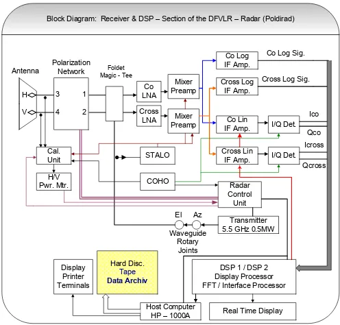
Fig. 1. Block diagram: receiver and DSP-section of the

DFVLR-Radar “Poldirad”.

With the good comparison results, we continued the work with the linear receiver data and started with the topic named “ temporal decorrelation properties of linear receiver weather radar data ”.

The temporal decorrelation properties, especially the decorrelation times of polarimetric weather radar echoes rep-resent an important property from the point of view of mea-surement accuracy of radar observables and their interpre-tation. For instance, the magnitudes of decorrelation times have a significant bearing on the choice of pulse repeat fre-quency and sample size and also in establishing the S-matrix coherence. Despite being a significant parameter in practi-cally all aspects of weather radar applications, it has met with unduly scant attention in the literature to date.

2 Radar specification and used archive data set

With refer to Fig. 1 and references Schroth et al. (1988) and Chandra et al. (1992), the specifications of the coher-ent polarimetric C-Band weather radar “Poldirad” are as follow: It is a C-band radar working with a tuneable fre-quency from 5.48 GHz to 5.85 GHz. There are three pos-sible radar impulse-volume range settings available. The range setting of 300 m leads to the unambiguous range of 300 km, the range setting of 150 m leads to the unambigu-ous range of 120 km and the high resolution range setting of 75 m leads to the unambiguous range of 60 km. The maximum available number of range bins is 452 and these range bins can be placed anywhere on the interval from 0 to 900 km, as long as the span from the first to the last range bin is less than 300 km. The dish antenna has an aperture

diameter of approximate 5 m with a focal length of approx-imate 4 m and an offset corrugated horn feed. The horizon-tal beamwidth is 1◦ _{with continuous scan and the vertical}

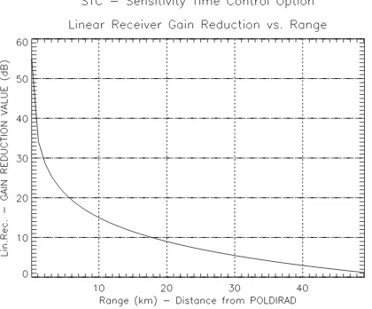
beamwidth is also 1◦ for the scan from –6◦ to 90◦. The gain of the antenna is approximate 44.5 dB and the side-lobe level of the pattern is less than –32 dB. The transmitter peak power is 400 kW, the pulse repeat frequency PRF is variable from 160 Hz to 2400 Hz (available settings: 160 Hz, 400 Hz, 800 Hz, 1200 Hz, and 2400 Hz) and the available pulse-width settings are 2µs, 1µs, and 0.5µs. The loss from the trans-mitter to the antenna feed is approximate 2.5 dB. The radar has two types of receiver, namely logarithmic and linear re-ceiver. The dynamic range of the logarithmic receiver is 80 dB and the dynamic range of the linear receiver is 60 dB. There are two receivers from each type available, so that there is a single receiver of each type for co- and cross- po-larized receive-channel. The linear receiver has two types of receiver gain control options available, the sensitivity time control (STC) option and the fixed gain option. The STC values are stored in the DSP in form of a look-up table and can be applied to IF amplifier with the range dependence of 1/R2, as shown in Fig. 2. In the fixed gain option, the radar operator has to choose the linear receiver gain reduction in according with the observed weather situation. Such as, in the strong weather situation one has to use lower receiver gain and in weak weather situation the receiver gain has to increase accordingly.

The radar can measure the reflectivity with accuracy less than±1 dB. The radial velocity and spectral width accuracy is better than±1 ms−1. The minimum detectable signal is –108 dBm, if a pulse with of 0.5µs is used. In reference Schroth et al. (1988) and Chandra et al. (1992) the radar spec-ification is discussed more detailed. Especially the linear and the logarithmic receiver behaviour is discussed in reference Chandra et al. (1992).

The archived data set used in this work was time series radar data (“Type 18”), which contains data from the linear and the logarithmic receivers for all range bins of the scan.

3 Theoretical Framework

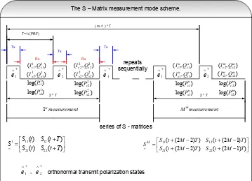
The radar provides transmission of general elliptical polar-ization stateeˆ₁+and T(T=1/PRF ) s later it transmitseˆ₂+ or-thogonal toeˆ+₁as shown in Fig. 3.

(3)

Fig. 2. Sensitivity time control (STC)-option dependence of the

linear receiver gain reduction vs. range.

unit for further processing. Please note that the logarithmic receivers work in parallel with the linear receivers, so that there is information from all linear and logarithmic receivers available for each transmitted impulse. One measurement consists of the transmission of two impulses with the two orthonormal transmission states and occurs over a time span of 2T, as shown in Fig. 3. The measurement is repeated sequentially with a predefined number of repetitions M (32, 64, 128). The results of one measurement with the two defined polarization states are for each transmission state the in-phase and quadrature voltage components from the linear receiver section for co- and cross- channel and for each transmission state the log measured power ( as voltage level ) from the logarithmic receiver section for co- and cross- channel. With this measurement mode scheme, the DSP then computes the results for all bins of the actual ray. A ray includes all range bins of one fixed azimuth and elevation angle. The type 18 datasets we used include the following measurement results for each single range bin of the whole scan.: from the linear receiver section we have the In-phase I and Quadrature-phase Q voltage components (no further processing by the DSP):

(I_cn₁, Qn_c₁), (I_xn₁, Qn_x₁), (I_cm₂, Qm_c₂),

(I_xm₂, Qm_x₂), n=1,3, ...,2M−1, m=2,4, ...,2M

and from the logarithmic receiver section we have the “effective reflectivity factor” (Battan, 1973) – pre processed by the DSP:

Zxx =10 log CR2Pxx[dBZ](3.1)

Zxy=10 log CR2Pxy

[dBZ](3.2) Zyx =10 log CR2Pyx[dBZ](3.3)

Zyy=10 log CR2Pyy[dBZ](3.4) ,

where M is the number of measurements, c1 denotes a co-polar component of the received signal with transmit

polarization 1, c2 denotes a co-polar component of the re-ceived signal with transmit polarization 2, x1 denotes a cross-polar component of the received signal with transmit cross- polar-ization 1, x2 denotes a cross-polar component of the received signal with transmit polarization 2, Z is the effective reflec-tivity factor (Battan, 1973) calculated by the DSP with xx .. yy denoting the transmit and receive states (e.g. xy: transmit state 1 receive state 2). Please note xx, yy are the co-polar results of the measurement and xy, yx are the cross-polar re-sults of the measurement. C denotes the radar constant saved in the DSP and R denotes actual range. With this information for every single range bin and additional information of the whole scan included in the data set type 18, we can continue with the post processing of the data. From the logarithmic receiver data we can derive some common weather radar pa-rameters, as there are the linear depolarization ratios LDR and the differential reflectivity ZDR. (These definitions are for H / V-transmit polarization states!)

LDRyx =10 log

_P

yx

Pxx

=Zxx−Zyx[dB](3.5)

LDRxy =10 log

_P

xy

Pyy

=Zyy−Zxy[dB](3.6)

ZDR=10 log _P

xx

Pyy

=Zyy−Zxx[dB](3.7)

From the linear receiver data the post processing is more complicated. For each measurement we have got eight values available, namely the co- and cross- polar quadrature volt-ages (I/Q) for each of the two transmit polarization states. For each bin we have got M measurements leading to a total number of M * eight values for each bin. The fact that linear receiver time series data lead to a huge amount of data and therefore to a huge amount of processing time and storage place, could be one reason why the linear receiver time series data is not used in common weather radar applications. But with the rapidly increasing processor speed and storage place of modern computers, this fact should be erased. Our start-ing point were the I and Q values, which were sampled and stored by the DSP. For each range bin we have a series of I and Q values, yielding to a series of in-phase and quadrature voltage components, that can be rearranged to the complex voltages as follows:

V_cn₁=I_cn₁+j Qn_c₁(3.8) V_xn₁=I_xn₁+j Qn_x₁(3.9) V_cm₂ =I_cm₂+j Qm_c₂(3.10) V_xm₂=I_xm₂+j Qm_x₂(3.11) n=1,3, ...2M−1 m=2,4, ...,2M ,

(4)

The S – Matrix measurement mode scheme.

T=1/(PRF)

Tx

Rx

2 * T

( m-1 ) * T

Tx Tx Rx repeats sequentially + ∧ 1

e e∧1+

+ ∧ 1 e + ∧ 2 e ) , ( 1 1 1 1 c c Q I ) , ( 1 1 1 1 x x Q

I ( , 2)

2 2 2 x x Q I ) , ( 2 2 2 2 c c Q

I ( ₂, m₂)

c m c Q I + ∧ 2

e (Imx2,Qxm2) )

,

( ₁ n₁

x n x Q I ) , (Icn1 Qcn1

2 * T

t measuremen Mth t measuremen st 1

series of S - matrices

      + + = ≈ () ( ) ) ( ) ( 22 21 12 11 1 T t S t S T t S t S S _      − + − + − + − + =

≈ ( (2 2) ) ( (2 1) )

) ) 1 2 ( ( ) ) 2 2 ( ( 22 21 12 11 T M t S T M t S T M t S T M t S SM + ∧ 1

e , e∧+2 orthonormal transmit polarization states

Each S – Matrix measurement occurs over a Time 2T, which for meteorological targets

should be less than the decorrelation Timeof the received echoes.

) log( ) log( 1 1 1 1 x c P P ) log( ) log( 2 2 2 2 x c P P ) log( ) log( 1 1 n x n c P P ) log( ) log( 2 2 m x m c P P

Fig. 3. S-Matrix measurement mode scheme.

a series of S-Matrix elements. By now we ignore the constant in the following formulas and include them at a later stage.

S₁₁n =const· V_cn₁(3.12) S₂₁n =const· V_xn₁

(3.13) S₁₂m =const· V_xm₂

(3.14) S₂₂m =const· V_cm₂

(3.15)

We now can combine the series of S-Matrix elements to a series of M S-Matrices. After this step of calculation, we can see the time slot of T between the S-Matrix columns, result-ing from the S-Matrix measurement mode scheme. This im-portant detail is also visible in Fig. 3. Each S-Matrix mea-surement occurs over a time span of 2T, which for me-teorological targets should be less than the decorrelation time of the received echoes!

SM =

S₁₁n S₁₂m S₂₁n S₂₂m

=

S_xxn Sm_xy S_yxn Sm_yy

(3.16)

With the obtained series of S-Matrices, we can now easily calculate common and new weather radar parameters. Our next step was the calculation of the Reflectivity LZ, the linear depolarization ratios LLDR and the differential Reflectivity LZDR for each range bin of the whole scan, with L denot-ing that the parameter was derived from the linear receiver

measurements.

LZxx=10 log CL1R2

SxxSxx∗

[dBZ](3.17)

LZxy=10 log

CL2R2

D SxySxy∗

E

[dBZ](3.18)

LZyx=10 log

CL2R2

D SyxS∗yx

E

[dBZ](3.19)

LZyy=10 log

CL1R2

D SyySyy∗

E

[dBZ](3.20)

LLDR1=10 logLZyx

LZxx

[dB](3.21)

LLDR2=10 logLZxy

LZyy

[dB](3.22)

LZDR=10 logLZxx

LZyy

[dB](3.23)

(5)

3.15). CL1/2=

λ2·Lt·CON ST1/2 Pt·τ·θ·φ·G2

(3.24)

where, λ-radar wavelength in cm, Pt-transmitted peak

power in kW, Lt-transmit loss, τ-pulse width in µs,

2/φ-horizontal/vertical half power full beamwidth, antenna gain and CONST includes all calculation constants. With the fac-tor CONST it is possible to have two radar constants, one for co-polar linear receiver channel and one for cross-polar lin-ear receiver channel. With the Eqs. (3.17 to 3.23) we have calculated parameters with the linear receiver data which should be equivalent to the parameters calculated by the DSP from the logarithmic receiver output. The comparison we have done is based on the DSP-products obtained from the logarithmic receiver and the results of the post processing of the linear receiver data (Eqs. 3.17 to 3.20). With the se-ries of S-Matrices we can now create the covariance matrix (Eq. 3.25) as a base for further calculations.

c=        

SxxSxx∗

D SxxSyx∗

E D SxxSxy∗

E D SxxSyy∗

E

SyxSxx∗

D SyxSyx∗

E D SyxSxy∗

E D SyxSyy∗

E

SxySxx∗

D SxySyx∗

E D SxySxy∗

E D SxySyy∗

E

SyySxx∗

D SyySyx∗

E D SyySxy∗

E D SyySyy∗

E         (3.25)

where, <> brackets indicate that the products of the S-Matrix elements (from each S-Matrix of the series of S-Matrices) is averaged over the number of measurements M and * denotes conjugate complex. Please note, that the elements of the main diagonal are real numbers. With this basis we now continue with the topic of temporal decorrela-tion properties of weather radar echoes.

Polarimetric measurements deliver S-Matrix measure-ments, which in general have S-Matrix columns that are decorrelated in time. This occurs because the two columns, depending on the measurement technique, are measure with a time difference of1t=1/PRF, as also illustrated in Fig. 3. It is therefore important that1t is smaller than the decorre-lation time in order for the measurements to be meaningful. Clearly this issue demands information regarding decorrela-tion times of precipitadecorrela-tion volume, with regard to precipita-tion intensity, precipitaprecipita-tion type and the polarizaprecipita-tion of the radar echoes. In this contribution we shall consider two cat-egories of parameter that help quantify decorrelation prop-erties. These parameter can be split into complex and real quantities and are defined as followed:

F12(1t )= ∞

R 0

f1(t )·f2(t+1t )dt

∞

R 0

f1(t )·f2(t )dt

(3.26)

where, f1and f2are real functions and1t is the time lag. The quantity above thus corresponds to autocorrelation if f1=f2, otherwise it corresponds to cross-correlation between f1and f2. For easier calculation, the denominator can be chosen to

be the autocorrelation of say f1. Likewise for the complex case we may define:

Z12(1t )= ∞

R 0

Z1(t )·Z∗₂(t+1t )dt

∞

R 0

Z1(t )·Z₂∗(t )dt

(3.27)

where, * again denotes conjugate complex. It may be noted that Z(1t) is now itself complex and thus contains informa-tion of relating to amplitude and phase decorrelainforma-tions sepa-rately. It may be important to distinguish between quantities called time decorrelation factor TDF and

decorrelation time DTτ. The decorrelation factor TDF is generally defined as:

T DF = F11(1t=2/P RF ) F11(1t=0)

·100[%](3.28)

For instance as used in the following Eqs. (3.29 to 3.32): T DFxx =

|hSxx∗(t )Sxx(t+2/P RF )i|

|hS∗

xx(t )Sxx(t )i|

·100[%](3.29) T DFxy=

D

S∗

xy(t )Sxy(t+2/P RF )

E D S∗

xy(t )Sxy(t )

E

·100[%](3.30)

T DFyx = D

S∗

yx(t )Syx(t+2/P RF )

E D S∗

yx(t )Syx(t )

E

·100[%](3.31)

T DFyy= D

S∗

yy(t )Syy(t+2/P RF )

E D S∗

yy(t )Syy(t )

E

·100[%](3.32)

We can calculate the time decorrelation factor for each ele-ment of the S-Matrix. It may be noted, that in the Eqs. (3.29 to 3.32) the<>brackets indicate that the products of the S-Matrix elements have to be averaged. In contrast the decor-relation time DTτ is given as the value of1t, here named as τ for which: (with e=2.718281 Euler constant)

F11(1t =τ ) F11(1t=0)

=e−1(3.33)

It may be noted, that we can define three types of decorre-lations, the first is magnitude decorrelation, second is power decorrelation and the third is the phase decorrelation. For these three types, we can calculate a decorrelation time. Fig-ure 4 shows an example for the Eq. (3.33).

(6)

Fig. 4. Correlation value vs. time lags (1 lag=2/PRF [s]).

(1): the mean life time of a particle before it breaks up or collides

(2): the velocity distribution of the particles in the impulse volume

(3): the turbulence in the impulse volume that imparts a random component in the velocities and last but not least the antenna rotation

At this stage of our work, we are making a quantitative assessment of the collective influence of all these aspects. With the exception of antenna rotation. This is true, because the data used was recorded with very slow antenna scanning speeds.

4 Results

First a few words to the database we have used. We have used archived datasets from the coherent polarimetric C-band weather radar “Poldirad” in Wessling (Germany), from the years 1987 to 1998. The available datasets cover all possible variations of the radar parameters like, pulse repetition fre-quency, pulse width, transmitted power, polarization bases and sample size. The basic specifications of the polarimetric weather radar “Poldirad” are given in Sect. 2. In this section we present the first results of our work, starting with the re-sults from the comparison of linear and logarithmic receiver signals of polarimetric weather radar echoes, followed by the results from the topic of temporal decorrelation properties of weather radar echoes. The results will be presented as fig-ures or tables with a short description in the following two Sects. 4.1 and 4.2. The discussion and interpretation of the results follows in Sect. 5.

4.1 Comparison of linear and logarithmic receiver signals of weather radar echoes

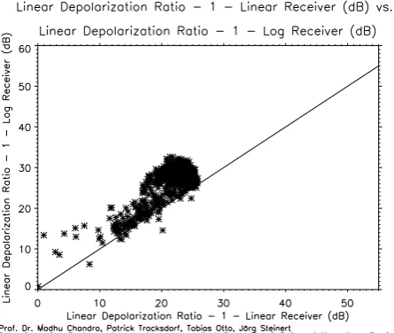
This section includes the results from the comparison of lin-ear and logarithmic receiver signals of polarimetric weather radar echoes. The results are presented in the Figs. 5, 6, 7 and 8. All these four figures are scatter-plots, where com-mon weather radar observables calculated from the logarith-mic receiver signals by the DSP are plotted against the corre-sponding weather radar observables we have calculated from the linear receiver signals. In each of the four plots, the x-axis is related to the observable obtained from the linear re-ceiver signals and the y-axis is related to the observable ob-tained from the logarithmic receiver signals. All four plots also include a “x=y”-line, so that a visual interpretation of the scatter-plots is possible. Figures 5 and 6 show the com-parison results for the weather radar observable “Reflectiv-ity”, where Fig. 5 shows the result for the co-polar receiver channel and Fig. 6 shows the result for the cross-polar re-ceiver channel. Figure 7 shows the comparison results for the weather radar observable “Linear Depolarization Ratio 2” and last but not least Fig. 8 shows the result for the weather radar observable “Differential Reflectivity”. The calculation procedures for the weather radar observables were given in the previous section.

4.2 Temporal decorrelation properties of weather radar echoes

(7)

Fig. 5. Reflectivity calculated with linear receiver data (x-axis) vs.

Reflectivity calculated by DSP with logarithmic receiver data (y-axis) the solid line: x=y line; result from the “co-polar receiver”; Basis transmit: V, receive: V.

the presented observable is “DTτxx”. The calculation proce-dures for the presented weather radar observables are again given in the Sect. 3. For completeness we can give the de-fined weather region as follows. In Figs. 9, 10, 11 and 12 we distinguish between the “melting band” and the “nor-mal weather region”, where the “nor“nor-mal weather region” can be split into the “weak weather situation” and the “strong weather situation”. In Tables 1 and 2 we distinguish between the “melting band” and again the “normal weather region”, but this time the “normal weather region” is split into “rain situation”, “snow situation” and “very weak weather situa-tion”. The defined weather regions are also discussed in the following section.

5 Discussion of the Results

In this section we discuss the results from the Sects. 4.1 and 4.2, starting again with the comparison of linear and logarith-mic receiver signals from polarimetric weather radar echoes. The results are shown in the Figs. 5, 6, 7 and 8. These four figures are obtained from one dataset. In Figs. 5 and 6 the reflectivity calculated from logarithmic receiver signal by the DSP is plotted against the reflectivity we calculated from linear receiver signals. Figure 5 shows the result for the co-polar receiver channel and Fig. 6 shows the result for the cross-polar receiver channel. As we can see from Figs. 5 and 6, there is a very good agreement between the reflectivi-ties calculated from logarithmic receiver signals by the DSP and reflectivities calculated from linear receiver signals. The solid line in Figs. 5 and 6 is the x=y line. The result for the co-polar receiver channel (Fig. 5) is more accurate then the result for the cross-polar receiver channel (Fig. 6). That’s due to the fact, that we used the same radar constant (Eq. 3.24)

Fig. 6. Reflectivity calculated with linear receiver data (x-axis) vs.

Reflectivity calculated by DSP with logarithmic receiver data (y-axis) the solid line: x=y line; result from the “cross-polar receiver”; Basis transmit: V, receive: H.

Fig. 7. LDR2 calculated with linear receiver data (x-axis) vs. LLDR2 calculated with logarithmic receiver data (y-axis) the solid line: x=y line; result from both co- and cross-polar receivers (see definition Eqs. 3.6, 3.22); Basis transmit: V/H, receive: V/H.

(8)

Fig. 8. LZDR calculated with linear receiver data (x-axis) vs. ZDR

calculated with logarithmic receiver data (y-axis) the solid line: x=y line; result from both co-polar and cross-polar receivers Basis trans-mit: V/H, receive: V/H.

-10 0 10 20 30 40 50

0 10 20 30 40 50 60 70 80 90

100 Decorrelation Factor vs. Reflectivity

Reflectivity (dBZ)

Decorrelation Factor (%)

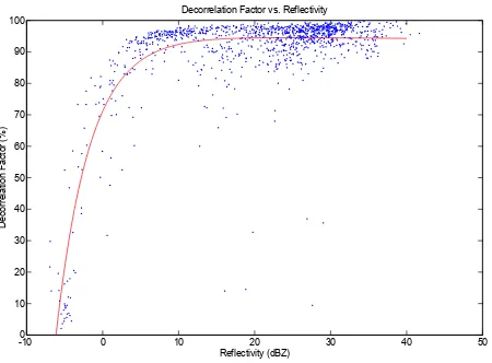
Fig. 9. Time decorrelation factor TDFxx (y-axis) vs. Reflectivity

(x-axis) red solid line – curve fit of the blue data points Basis

trans-mit: V, receive: V; PRF: 1200 Hz; PW: 1µs; Sample Size: 128.

linear depolarization ratio LDR2 calculated from logarithmic receiver signals with LLDR2 calculated from linear receiver signals. Again there is a good agreement between the observ-ables LDR2 and LLDR2 calculated from logarithmic and lin-ear receiver signals. Figure 8 shows the comparison for the differential reflectivity ZDR, again with a good agreement. This observation is consistent with the statistical properties of the linear and logarithmic radar echoes. With the results in Figs. 5, 6, 7 and 8 we have done the comparison of linear and logarithmic receiver signals for common weather radar observables with good agreement. We can conclude, that the linear receiver data is accurate in comparison to the logarith-mic receiver data and that we can use it for weather radar data

Fig. 10. Decorrelation Time DTτxy(y-axis) vs. Reflectivity (x-axis)

Basis transmit: V, receive: H; PRF: 1200 Hz; PW: 1µs; Sample

Size: 128, red data points belong to the melting band/solid lines: curve fit of plot .

Fig. 11. Decorrelation Time DTτxy(y-axis) vs. Reflectivity (x-axis)

Basis transmit: V, receive: H; PRF: 1200 Hz; PW: 1µs; Sample

Size: 128, red data points belong to the melting band/solid lines: curve fit of plot.

analysis. The fact, that the linear receiver data also provides phase information, opens a wide field for new approaches in weather radar data analysis.

(9)

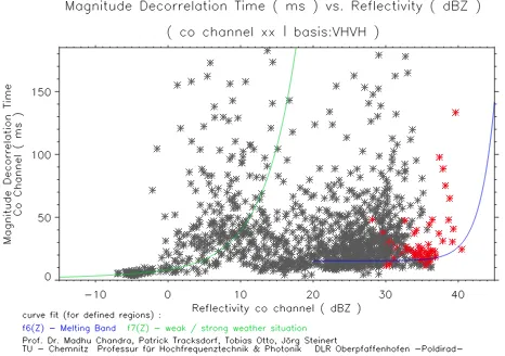
Fig. 12. Decorrelation Time DTτxx(y-axis) vs. Reflectivity (x-axis)

Basis transmit: V, receive: V; PRF: 1200 Hz; PW: 1µs; Sample

Size: 128, red data points belong to the melting band/solid lines: curve fit of plot .

f (Zxx)=95.17∗exp(−0.0002341∗Zxx)

−24.07∗exp(−0.2242∗Zxx) (5.1)

For small reflectivities (–10 dBZ to 5 dBZ ) the time decor-relation factor TDF is increasing very rapidly and for higher reflectivities (5 dBZ to 40 dB) the time decorrelation factor TDF is not stationery but very slowly increasing to 100%. Small reflectivities indicate a very weak weather situation with few moving particles in the observed range bin and therefore the two pulse lag (1t=2/PRF)-correlation value will be small. Also the noise takes place in a weak weather situation, which has a negative influence on the two pulse lag correlation value. With increasing number of moving parti-cles (stronger weather situation) the reflectivity will increase. The random media in the observed range bin has now more reflecting particles, that leads to the result, that the noise loses its influence and that the two pulse lag-correlation value will be stronger. In strong weather situation the range bin is randomly filled with lots of moving particles, that lead to a strong two pulse lag-correlation value, which is increasing slowly to 100% with increasing reflectivity. These consid-erations also suggest that stronger rain volumes, apart from having more numerous raindrops in the active volume, also have a more monodisperse distribution of the particles.

In Figs. 10 and 11 we can see the decorrelation time DTτxy

from the cross-polar linear receiver channel plotted against the reflectivity from the cross-polar linear receiver channel. The used transmit polarization state was vertical and the re-ceive polarization state was horizontal. The Figs. 10 and 11 show the same data but the application of the curve fitting is different. These plots were obtained with the real calcula-tion method (Eq. 3.26) and this decorrelacalcula-tion time is based

on magnitude. Therefore we can give the formula for f1and f2as follows:

f1(t )=f2(t )=( Sxy(t )

) (5.2)

and complete the name to magnitude decorrelation time mDTτxy. The same definition for f1 and f2 was also used for the basis of Table 2. From Figs. 10 and 11 we can see that for very small reflectivities (–10 dBZ to 2 dBZ) the cal-culated decorrelation times are small and increasing slowly. Small reflectivities are again related to weak weather situ-ation, the random media is filled with few moving particles and the noise gains influence. Here, the movement of the few particles have a larger effect on the correlation value. That will cause the correlation value to drop fast below the value of e−1and therefore the decorrelation time will be smaller. For higher reflectivities (2 dBZ to 11 dBZ) the decorrelation times are increasing very rapidly. This behavior is as ex-pected, because in strong weather situations (higher reflectiv-ities) the random media is randomly filled with lots of mov-ing particles, noise loses its influence and therefore the decor-relation times should be higher. The movement of the many particles have a smaller effect on the correlation value and it drops slower below the value of e−1. The red data points in Figs. 10 and 11 belong to the melting band. We can see that the data points which belong to the melting band have high reflectivity values (11 dBZ to 28 dBZ) but significantly smaller magnitude decorrelation times. For the melting band we can say that it is more turbulent and therefore the decorre-lation times, even if the reflectivities are stronger, are smaller then in other regions with high reflectivities. We have used the least mean square method (LMS) of curve fitting to find the corresponding mathematical relationships between the magnitude decorrelation time and reflectivity for the defined regions. As a first step (Fig. 10) we decided to distinguish between the melting band and the “normal weather region” (which includes weak and strong weather situations). The curve fitting for the melting band can be seen in Fig. 10 as a blue solid line. The following formula gives the result from curve fitting for the melting band as an exponential curve: f1(Zxy)= −33.5275∗exp(0.04311∗Zxy)

+14.6644∗exp(0.0694∗Zxy)+37.8688(5.3)

The curve fitting for the “normal weather region” can be seen in Fig. 10 as a light green solid line. The following formula gives the result from curve fitting for the “normal weather region” as an exponential curve:

f2(Zxy)=1.3814∗exp(0.5036∗Zxy)

−0.3583∗exp(0.5036∗Zxy)+5.1783(5.4)

(10)

gives the result from curve fitting for the melting band as an exponential curve: (same as Eq. 5.3)

f3(Zxy)= −33.5275∗exp(0.0431∗Zxy)

+14.6644∗exp(0.0694∗Zxy)+37.8688(5.5)

The curve fitting for the “weak weather region” can be seen in Fig. 11 as a green solid line. The following formula gives the result from curve fitting for the “weak weather region” as an exponential curve:

f4(Zxy)=2.5269∗exp(0.5284∗Zxy)

−1.4995∗exp(0.5384∗Zxy)+5.1798(5.6)

The curve fitting for the “strong weather region” can be seen in Fig. 11 as a dark green solid line. The following formula gives the result from curve fitting for the “strong weather region” as an exponential curve:

f5(Zxy)=(1.72715e−10)∗exp(3.3579∗Zxy)

−88.2583∗exp(0.0895∗Zxy)−89.2516(5.7)

In Fig. 12 we can see the decorrelation time DTτxxfrom the

co-polar linear receiver channel plotted against the reflectiv-ity from the co-polar linear receiver channel. The used trans-mit polarization state was vertical and the receive polariza-tion state was vertical (co-polar). This plot was also obtained with the real calculation method Eq. (3.26) and this decorre-lation time is based on magnitude. For the co-polar case we can give the formula for f1and f2as follows:

f1(t )=f2(t )=(|Sxx(t )|) (5.8)

and complete the name to magnitude decorrelation time mDTτxx. The same definition for f1 and f2 was also used for the basis of Table 1. The red data points in Fig. 12 belong to the melting band. Again we distinguished between the melting band and the “normal weather region”. The curve fitting for the “melting band” can be seen in Fig. 12 as a dark blue solid line. The following formula gives the result from curve fitting for the “melting band” as an exponential curve: f6(Zxx)=(−3.2734e−11)∗exp(0.4494∗Zxx)

+(3.4861e−8)∗exp(0.4892∗Zxx)+15.43(5.9)

The curve fitting for the “normal weather region” can be seen in Fig. 12 as a green solid line. The following formula gives the result from curve fitting for the “normal weather region” as an exponential curve:

f7(Zxx)=3.6459∗exp(0.2202∗Zxx)

−332.2287∗exp(−0.00051∗Zxx)+336.9638(5.10)

The wide scatter of the data points in Fig. 12 reflects the need to consider separating the points further, i.e., on the basis of weather type, range, power level and doppler spread.

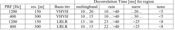
Tables 1 and 2 contain the empirical results from several datasets for magnitude decorrelation time vs. reflectivity in predefined regions. We decided to split the results for co-polar channel results (Table 1) and cross-co-polar channel re-sults (Table 2). The regions have been defined with the help of the related reflectivity-plot (the whole dataset). We col-lected empirical results for two polarization bases and for each of the two polarization bases we decided to take two different range resolutions (basis notation: transmit1, trans-mit2, receive1, receive2). What can be seen as a whole from Tables 1 and 2 is, that with increasing range resolution (and increasing PRF) the magnitude decorrelation times also in-crease. In region “none” with weak weather situation or no weather situation at all (very small reflectivities), it can be seen, that the magnitude decorrelation times are small. The highest magnitude decorrelation times appear in the rain and heavy rain situation. From Tables 1 and 2 it can be seen, that the magnitude decorrelation times for the melting band are smaller than the magnitude decorrelation times for the rain and heavy rain situation (although the reflectivities in the melting band are higher). There is a small difference in mag-nitude decorrelation times for different polarization bases.

6 Conclusion

(11)

Table 1. Empirical results: Decorrelation Time DTτxx for defined regions, results from co-polar linear receiver channel; real calculation

method multiple scans as empirical basis; res. = range resolution.

12 1

2

Figure 12: Decorrelation Time DTτxx (y-axis) versus Reflectivity (x-axis)

3

Basis transmit: V, receive: V; PRF: 1200 Hz; PW: 1µs; Sample Size: 128 4

red data points belong to the melting band / solid lines: curve fit of plot 5

6

Decorrelation Time [ms] for region PRF [Hz] res. [m] Basis ttrr meltingband rain snow none

1200 150 VHVH 10 .. 20 21 .. >40 >20 n.a. 400 300 VHVH 10 .. 18 18 .. >40 20 .. 40 <10 1200 150 LRLR 13 .. 20 22 .. >40 >20 <10 400 300 LRLR 10 .. 15 15 .. >40 18 .. 20 <10 7

Table 1: empirical results: Decorrelation Time DTτxx for defined regions,

8

results from co-polar linear receiver channel; real calculation method 9

multiple scans as empirical basis; res. = range resolution 10

11

1200 150 VHVH 10 .. 20 10 .. >40 .. 20 .. <5 400 300 VHVH 10 .. 15 10 .. >40 .. 30 .. <5 1200 150 LRLR 13 .. 16 23 .. >40 >25 <8 400 300 LRLR 10 .. 15 22 .. >40 >25 <8 12

Table 2: empirical results: Decorrelation Time DTτxy for defined regions,

13

results from cross-polar linear receiver channel; real calculation method 14

Table 2. Empirical results: Decorrelation Time DTτxyfor defined regions, results from cross-polar linear receiver channel; real calculation

method multiple scans as empirical basis; res. = range resolution.

12 1

2

Figure 12: Decorrelation Time DTτxx (y-axis) versus Reflectivity (x-axis)

3

Basis transmit: V, receive: V; PRF: 1200 Hz; PW: 1µs; Sample Size: 128 4

red data points belong to the melting band / solid lines: curve fit of plot 5

6

1200 150 VHVH 10 .. 20 21 .. >40 >20 n.a. 400 300 VHVH 10 .. 18 18 .. >40 20 .. 40 <10 1200 150 LRLR 13 .. 20 22 .. >40 >20 <10 400 300 LRLR 10 .. 15 15 .. >40 18 .. 20 <10 7

Table 1: empirical results: Decorrelation Time DTτxx for defined regions,

8

results from co-polar linear receiver channel; real calculation method 9

11

1200 150 VHVH 10 .. 20 10 .. >40 .. 20 .. <5 400 300 VHVH 10 .. 15 10 .. >40 .. 30 .. <5 1200 150 LRLR 13 .. 16 23 .. >40 >25 <8 400 300 LRLR 10 .. 15 22 .. >40 >25 <8 12

Table 2: empirical results: Decorrelation Time DTτxy for defined regions,

13

results from cross-polar linear receiver channel; real calculation method 14

range resolutions. The reported work should enable future applications which combine polarimetric observations with temporal properties of the multi-channel radar echoes. The study also suggests further investigations to assess the rel-ative influences of other radar parameters on the temporal properties of radar signals. As already indicated earlier, these parameters include: (1) the Doppler spectrum of the target, (2) the size of the impulse volume, (3) the range dependence, (4) the hydrometeor size-distribution, and (5) the signal-to-noise ratio.

References

Battan, L. J.: Radar Observation of the Atmosphere, The University of Chicago Press, 1973.

Bringi, V. N. and Chandrasekar, V.: Polarimetric Doppler weather radar Principles and Applications, Cambridge University Press, 2001.

Chandra, M., Clemens, E., Ritenberg, F., Schnabl, G., Schroth, A., and Tragl, K.: Polarimetric Meteorological Instrumentation Radar Facility, Direct and Inverse Methods in Radar Polarime-try, part 2, edited by: Boerner, W. M. et al., Kluwer Academic Publishers, 1579–1612, 1992.

Schroth, A., Chandra, M., and Meischner, P.: A C-Band Coherent Polarimetric Radar for Propagation and Cloud Physics Research, Journal Of Atmospheric And Oceanic Technology, Volume 5, 803–822, December 1988.