REVIEW
A survey of submesoscale currents
James C. McWilliams
*Abstract
Submesoscale currents are pervasive throughout the ocean. They have intermediate space and time scales—neither mesoscale nor microscale—that have made them elusive for measurements and modeling until recently. In this brief article, a survey is presented of their primary characteristics and interpretive explanations, intended for a broad audience of physical and biogeochemical oceanographers. Besides their identifying scales, submesoscale currents are distinctive in their flow patterns, their essential dynamical processes, and their consequences for transport, mixing, and dissipation in the general circulation. There are two primary submesoscale populations, a frontal one in the near-surface layer with its typically reduced stratification, and another vortical one, generated in topographic wakes, that (sparsely) fills the oceanic interior.
Keywords: Submesoscale currents, Density fronts and filaments, Coherent vortices, Topographic waves
© The Author(s) 2019. This article is distributed under the terms of the Creative Commons Attribution 4.0 International License (http://creat iveco mmons .org/licen ses/by/4.0/), which permits unrestricted use, distribution, and reproduction in any medium, provided you give appropriate credit to the original author(s) and the source, provide a link to the Creative Commons license, and indicate if changes were made.
Introduction
The ocean is highly variable: just ask any sailor or sea-going experimentalist. Among its modes of variability is a class of phenomena that have come to be called sub-mesoscale currents (abbreviated here as SMCs). The SMC name arose in relation to the widely familiar mesoscale eddies that contain the greatest fraction of kinetic energy in the ocean; i.e., SMCs are the next size class down from the eddies, with typical horizontal lengths of tens to ten thousands of meters, vertical heights of ten to hundreds of meters, and evolutionary time scales of hours to days.1
The name is also apt in the sense that the primary source for SMC energy comes from mesoscale eddies by a down-scale transfer. The principal SMC generation mechanisms are (1) extraction of available potential energy (due to hori-zontal buoyancy gradients) in the weakly stratified surface layer either through baroclinic instability or frontogen-esis, and (2) topographic-drag vorticity generation in flows along a sloping bottom, followed by boundary current separation and wake instability. These phenomena partly manifest a loss of hydrostatic, geostrophic momentum bal-ance, and they exhibit a turbulent energy cascade forward toward even smaller scales. Thus, SMC dynamics typi-cally go beyond quasigeostrophy, which is the generally
successful theoretical framework for mesoscale eddies, while still being strongly influenced by Earth’s rotation and the generally stable density stratification in the ocean. That is, the Rossby and Froude numbers:
are typically order-one parameters, rather than their usually small values for mesoscale eddies (V is a charac-teristic horizontal velocity scale, ℓ and h horizontal and
vertical length scales, f the Coriolis frequency, and N the Brunt–Vaisala or stratification frequency.) Thus, a Rossby number Ro measures the relative magnitude of momen-tum advection relative to the Coriolis force, and a Froude number Fr measures the ratio of an advecting velocity to the phase speed of an internal gravity wave. Small values for these numbers indicate the dynamical importance of rotation and stratification. Nevertheless, the evolution of SMCs is primarily through advection, which distin-guishes it from the inter-gravity waves that can occupy similar scale ranges in the ocean; their mutual influence is a topic of current research, but, in some first approxi-mation, their interactions are weak.
The science of SMCs has blossomed in recent years. The delay, compared to other more familiar types of (1)
Ro= V
fℓ and Fr=
V Nh,
Open Access
*Correspondence: jcm@atmos.ucla.edu
Department of Atmospheric and Oceanic Sciences, UCLA, 405 Hilgard Ave., Los Angeles, CA 90095-1565, USA
Page 2 of 15 McWilliams Geosci. Lett. (2019) 6:3
oceanic currents, is mainly due to technical barriers. The SMC space and time scales are awkwardly in between the finer scale sampling from ships, sparse buoys, and floats, and the larger scale sampling from most satellite sensors; their simulation requires large computations that encompass both the mesoscale and submesoscale ranges; and the relevant theories involve difficult nonlin-ear dynamics. The more recent empowering technologies are high-resolution surface images, multiply-nested com-putational simulation methods, and, in a few instances, massive swarms of surface drifters (as in the CARTHE experiments in the Gulf of Mexico). As yet there is no widely deployable SMC measurement technique for the subsurface ocean, so simulations are leading the way. Autonomous gliders and ship-towed instruments can provide submesoscale spatial sampling along their tracks, but they are limited to two dimensions and thus often have difficulty in distinguishing SMCs and inertia-gravity waves.
Figure 1 is diagram of the flow of information and energy in the global oceanic circulation.2 Their
origi-nating source is forcing by surface winds and air–sea
buoyancy fluxes at the energetic scales of the atmos-phere, i.e., mostly on the planetary scale comparable to the size of oceanic basins. The direct oceanic response is oceanic currents on the basin and inter-basin scales, including their narrower transport closures as boundary and equatorial currents. On the other hand, the sink is energy dissipation and information loss that can only be completed at the microscale due to molecular viscosity and conductivity. Currents of different types must con-nect the source and sink across the intervening scales and dynamical regimes. The first step is geostrophic instabili-ties of the forced circulation, yielding mesoscale eddies. Through the force-balanced constraints of geostrophic and hydrostatic balance, they are inhibited from further transfers to smaller scales; i.e., they have an inverse cas-cade of energy (Charney 1971). Leakages out of the mes-oscale eddies by partial violation of these force balances continue downscale. Three middle-scale “routes” are depicted in Fig. 1: (1) spontaneous emission of inertia-gravity waves from currents, either in the interior or as bottom lee waves, followed ultimately by energy transfer to smaller scales; (2) partly ageostrophic instabilities and forward energy cascade of non-wave (partly balanced) currents; and (3) turbulent bottom drag on currents that generates both bottom boundary-layer turbulence Fig. 1 Stages in the oceanic general circulation from planetary scale forcing to microscale dissipation and mixing: climate forcing by wind stress and air-sea buoyancy flux; balanced flow dynamics (e.g., mostly geostrophic and hydrostatic); submesoscale transitional dynamics; and microscale flows with only a weak influence from Earth’s rotation, a mostly unbalanced momentum dynamics with large accelerations, and an approximate equivalence of vertical and horizontal lengths scales, h∼ℓ . The Rossby and Froude numbers, Ro and Fr, start from very low values at the planetary scale, pass through O(1) values within the submesoscale regime, and end up with large values at the microscale
and topographic vortical wakes. Below this middle-scale range, three-dimensional turbulence completes the con-nection to the microscale. While no accurate global accounting of these three routes is yet available, the SMC role in the latter two routes is almost certainly a domi-nant one. Along the pathway toward the microscale, the character of the currents changes from being highly anisotropic with h/ℓ≪1 and relatively small vertical velocity to approaching isotropy with h∼ℓ , as in
Kol-mogorov’s paradigm for universal turbulent behavior at high Reynolds number. In addition, the local Ro and Fr
systematically increase as h and ℓ decrease.
The paper is organized by considering the two SMC surface-layer and topographic populations separately in “Lines on the surface” and “Topographic wakes” sections, and it ends with a summary in “Final remarks” section.
This article is adapted from a lecture given at the 2018 annual meeting of the Asia Oceania Geosciences Society (AOGS) in Honolulu, HI. It is intended for a broad audi-ence, and it is more about my experiences and opinions, with some illustrations, rather than about the full evidence and literature behind them. A more extensive and schol-arly review article is McWilliams (2016), while this paper is intended to complement it for a more general audience.
Lines on the surface
SMCs can be difficult to discern in single vertical profiles or time series because of potential confusions with other types of flows. Among the most useful observations are surface images, especially those with high horizontal res-olution (subsurface images are rare, but see Fig. 14). By the addition of an extradimension and with dense sam-pling, patterns emerge, and with experience, they can be interpreted for their underlying phenomena. Images in a horizontal plane (i.e., at the oceanic surface) allow a recognition of sharp convergence lines and small, hori-zontally recirculating vortices. Several examples are pre-sented in this section.
Besides the recognition of lines of large horizontal den-sity gradients (i.e., fronts), many of these lines exhibit meanders, which is suggestive of frontal instability, likely due to the associated vertical or horizontal shear in the mixed layer. The former is a type of baroclinic instabil-ity but with preferred length scales that are in the sub-mesoscale range due to the small surface-layer baroclinic deformation radius (Boccaletti et al. 2007; Fox-Kemper et al. 2008). The latter is a form of classical shear insta-bility that is engendered by the sharpening horizontal gradients caused by active frontogenesis. Both types can be partly ageostrophic because of the large value of the Rossby number.
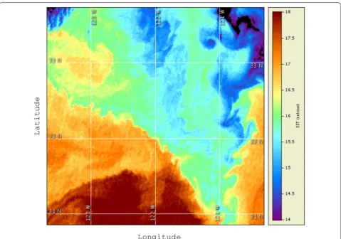
A snapshot of sea surface temperature (SST) within the California Current System shows both mesoscale eddies
and associated submesoscale fronts, filaments, instabili-ties, and vortices (Fig. 2). A front is defined as a sharp horizontal gradient in density with an extensive central axis in the perpendicular direction (i.e., a line along the surface). A filament is similar, except that it is a narrow horizontal extremum in density. Both light and dense filaments are possible, but dense filaments have much stronger ageostrophic circulation and more rapid fron-togenesis, and, hence, are more common in the ocean (McWilliams et al. 2009; Adams et al. 2017). These sub-mesoscale density patterns have associated geostrophic flows along the axis and ageostrophic flows, especially in the cross-axis plane.
A sun-glint reflection pattern in the Mediterranean Sea (Fig. 3) reveals a dense family of lines on the sur-face. They are due to high concentrations of buoyant surfactants (in this case biogenic scum) that are gath-ered into narrow lines along the front or filament axes by surface ageostrophic convergence with downwelling jets underneath. The surrounding submesoscale flows give a pattern organization to the lines, thus serving as a means of flow visualization. In this example, at least two scales of SMCs are present. The larger scale of kilometers is a vortex street of a sort which one might plausibly associ-ate with the lassoci-ate stage of an instability of a lassoci-ateral shear layer. The smaller scale of tens to hundreds of meters is the lines themselves. Within the vortices, the lines have an inwardly spiraling pattern that exposes both cyclonic swirl and a central convergence in the vortex cores. This led Walter Munk to refer to these as “spirals on the sea” (Munk et al. 2000). During the manned space flight era, many examples were photographed by the astronauts. Outside the vortices, the lines indicate a generally larger scale (mesoscale) flow pattern.
A closer view of an SMC convergence line is in Fig. 4, a photograph taken from a ship in the Gulf of Mexico. Here, it is floating seaweed that is gathered along the axis. The cross-line scale is a few tens of meters, and the along-axis scale reaches to the horizon. This example is from a study whose main content was satellite images showing a dense network of such lines spanning a wide region of hundreds of kilometers in the central Gulf of Mexico (Gower et al. 2006).
Page 4 of 15 McWilliams Geosci. Lett. (2019) 6:3
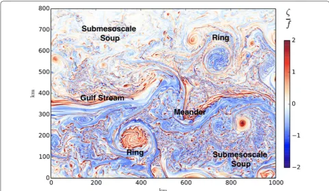
vermicelli in mind (e.g., the regions away from the Gulf Stream in Fig. 6).
Such images and photographs are highly informative, but their information is intrinsically subjective. It is quite difficult to get in situ measurements that cover the indi-cated patterns, though there have been some successes. More generally, however, the quantitative science of SMCs has been advanced by computational simulations. An example for the offshore Gulf Stream is Fig. 6. The experience has been that, in realistic simulations with active mesoscale eddies and associated horizontal den-sity gradients, a sufficiently fine-grid resolution will lead to the spontaneous emergence of SMCs that first arise in the weakly stratified surface layer. The necessary resolu-tion varies with condiresolu-tions (e.g., region or season), but it is around dx≈1 km; such simulations can be referred to
as “submesoscale-permitting”, because the full range of submesoscale variability extends down to ≈ 10–100 m, and the latter would have to be reached to be fully “sub-mesoscale-resolving”. Nevertheless, simulations show
approximately self-similar scaling behavior when dx is varied within this submesoscale range. The associated kinetic-energy horizontal-wavenumber spectra are rela-tively shallow, E(k)∼k−γ , with γ ≈2 , where k is the
horizontal wavenumber. This differs from simulations and altimetric sea-level measurements that show gen-erally steeper spectra (larger γ values) in the mesoscale range. The value of the simulation results is mainly in the phenomenological discoveries they have enabled. This is illustrated in Fig. 6 by the variety of different SMC pat-terns associated with different mesoscale environments. Once the phenomenology is known, then detailed diag-nostic analyses and theoretical explanations can be adduced.
reach scales where rotation and stratification influences cease to be significant (i.e., relevant Ro and Fr values are large; Sullivan and McWilliams 2018). Both estimates would yield a horizontal scale in the 10–100 m range. Whether, in fact, there are important non-hydrostatic effects on SMCs at larger scales remains to be further tested.
In the surface layer, the principal energy source for SMCs is the available potential energy associated with horizontal density gradients on larger scales.
This energy source can be tapped either by baroclinic instability (often called mixed-layer instability when confined to the weakly stratified surface layer) or by frontogenesis. Frontogenesis is a familiar concept from meteorology because of its frequent manifesta-tion on surface weather maps. The prevailing mete-orological interpretation is that fronts are caused by the horizontal strain rate in what is called a deforma-tion flow (e.g., confluence in a horizontal plane) on a larger scale. A sketch of the associated surface frontal structure is in Fig. 7 for both density-front and dense-filament configurations. The horizontal buoyancy (i.e.,
b= −gρ/ρ0 , where g is gravity, ρ is density, and ρ0 a
mean value) gradient will initially sharpen at an expo-nential rate ∼exp[αt] as a function of time t, if the gra-dient is favorably aligned in relation to a barotropic deformation flow with a uniform strain rate, no hori-zontal divergence, and no vorticity; i.e., u=(ud,vd, 0)
with ud = −αx/2 and vd= αy/2 , where α is the hori-zontal strain rate and (x, y, z) and (u, v, w) are the
coor-dinates and velocity components in the (east, north, and upward) directions (Fig. 7a). Because of this den-sity structure, there is an associated circulation, both along the axis and mostly geostrophic in v, and in the cross-axis plane with ageostrophic u and w. If the front is uniform along the axis or if an average is taken in this direction (denoted by angle brackets), then the cross-axis velocity is 2D non-divergent, and it can be repre-sented with a secondary-circulation streamfunction defined by the following:
Fig. 3 Spirals on the sea. Sun-glint pattern in a photograph by an astronaut Scully-Power (1986) over the Mediterranean not far off the coast of North Africa. The lines are created by surfactants concentrated in convergence lines that alter the scattered reflection by short-surface gravity waves. Their patterns are organized by submesoscale currents. The vortex diameters are ≈ 5 km, and the surfactant lines are ≈ 100 m wide. The pattern suggests that a vortex-street roll-up has occurred from a lateral shear instability of some antecedent front, filament, or headland wake
Fig. 4 Surface convergence line. A fantail view of a ≈ 10 m-wide line of buoyant sargassum weed in the Gulf of Mexico concentrated by a submesoscale frontal secondary circulation (Gower et al. 2006). Notice the along-front extent away into the distance, with a suggestion of frontal meanders or instabilities
Page 6 of 15 McWilliams Geosci. Lett. (2019) 6:3
For a front, is a positive monopole indicating a closed
circulation loop with upwelling on the light side and sur-face flow toward the dense side. For a dense filament, is
a dipole, with strong central downwelling. Both patterns imply that wb>0 , i.e., the conversion of available
poten-tial energy to the SMC kinetic energy. Once ∇b is strong enough, and is large enough, then the frontogenetic
rate increases due to surface horizontal convergence of the secondary circulation, − �ux� > 0 , and it further
amplifies until some other process arrests the frontogen-esis. The frontal arrest process (discussed at the end of this section) sets the lower size limit for SMCs.
Strain-induced frontogenesis can occur in the ocean, with the principal strain and buoyancy gradients asso-ciated with mesoscale eddies or strong currents. More commonly in simulations, however, the dynamical character of the submesoscale fronts is consistent with a combination of a surface density gradient and vertical momentum mixing by boundary-layer turbulence. This situation is called Turbulent Thermal Wind (TTW), which has a linear, steady, surface-layer, incompressible
(2)
(�u�, �w�)=(−∂z, ∂x)�. approximation in its horizontal momentum and conti-nuity balances:
where νv is the vertical eddy viscosity associated with
boundary-layer turbulence. Without the buoyancy gradi-ent, this would describe an Ekman layer. Without the tur-bulent mixing, it would describe a geostrophic current in thermal wind balance. Together, they describe the mixed geostrophic and ageostrophic currents associated with a given ∇b and νv (McWilliams 2017). The TTW b and fields for a surface front are shown in Fig. 8. Interest-ingly, the monopole pattern is qualitatively the same as for a front in a deformation flow (Fig. 7), and the same similarity occurs for dense filaments. Thus, the TTW cir-culations are also frontogenetic due to the surface con-vergence on the dense side or center. The last panel in
(3) −∂z[νv∂zu] − fv= − ∂x
z
bdz
−∂z[νv∂zv] +fu= − ∂y z
bdz
∂xu+∂yv+∂zw=0 ,
Page 8 of 15 McWilliams Geosci. Lett. (2019) 6:3
Fig. 8 shows the Lagrangian tendency for the SMC hori-zontal shear variance, Tu = D|∇u|2/Dt : it is strongly
positive on the upper dense side of the front. Thus, dif-ferential advection by the secondary circulation is the
cause of frontogenesis in both the buoyancy gradient and velocity shear.
The simulations discussed above are made with what is called a oceanic circulation model, designed to calcu-late currents on larger scales, starting from global and Fig. 8 Frontogenesis by turbulent thermal wind (TTW). The buoyancy field b (left), ageostrophic secondary-circulation streamfunction (center), and Lagrangian, velocity-gradient frontogenetic tendency, Tu
= D|∇u|2
/Dt [10−13 s −3 ] (right), for an idealized 2D surface front with vertical mixing (McWilliams 2017). The thick black line, pointed to by the arrow on the left panel, is the boundary-layer depth, and the curved line in the center panel indicates the direction of the secondary circulation. The horizontal convergence on the dense side near the surface (i.e., the upper left region in the buoyancy b(x, z) in left panel induces frontogenesis in both ∇b and ∇u
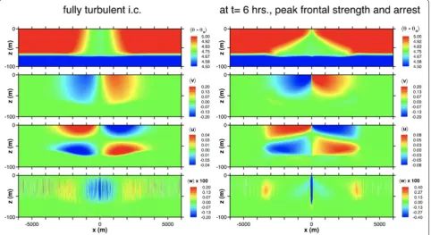
Fig. 9 Simulated filament frontogenesis by TTW. A fully turbulent “initial condition” (left) and 6 h later at the time of peak frontal strength and frontal arrest (right), in a Large-Eddy Simulation (LES) of a submesoscale dense filament in a boundary layer with surface cooling (Sullivan and McWilliams 2018). The (x, z) fields are averaged in the along-front y direction: temperature �θ� −θ0 , along-front velocity v , cross-front velocity u , and vertical velocity w . Units are ◦ C and m s −1 , respectively. The apparent noise in w is sampling error due to the finite domain size in y and the presence of
working downward as computational capacity allows. Most circulation models make the hydrostatic approxi-mation, which seems generally safe to within the sub-mesoscale-permitting regime, apart from whatever high-frequency internal gravity waves might arise. In such a model, small-scale turbulent mixing is parameter-ized, as with the vertical eddy viscosity νv in (3).
Some-where approaching the dynamical microscale, however, the validity of these simplifications will fail. A dynami-cal model that is more complete is dynami-called a Large-Eddy Simulation (LES), e.g., commonly used for turbulent boundary layers. With respect to SMCs, a large LES cal-culation that includes both a SMC and its microscale tur-bulence is a valuable tool for a more fundamental view of their mutual interaction. The following figures are taken for such an LES simulation (Sullivan and McWil-liams 2018). It is posed for an isolated dense filament in an otherwise turbulent boundary layer (e.g., due to a sur-face wind stress and/or convective buoyancy flux). This is a TTW frontogenetic situation. Figure 9 shows the LES initial conditions for the along-axis-averaged tem-perature (buoyancy) and velocity field in the presence of a fully developed, turbulent, convective boundary layer. Their structure is similar to the filament structure in Fig. 7. From this state, rapid frontogenesis ensues, as seen
in the same figure at a time 6 h later. The filament width has narrowed dramatically at the surface while broaden-ing deeper in the layer. The velocity patterns are similar to their initial shapes, but deformed to have very sharp near-surface gradients at the filament center. In particu-lar, the central w<0 jet has amplified and narrowed substantially. Another view is provided by the cross-axis streamfunction (Fig. 10), whose horizontal convergence in the center similarly narrows and amplifies in accom-paniment to the frontogenesis. The time of 6 h coincides with the peak frontal strength as measured by both the vertical vorticity, �ζ� =∂x�v� , and the downward jet, w (Fig. 11). The duration of the frontogenesis period
depends on how strong and wide the filament buoyancy gradient is initially and on the strength of the turbulent momentum mixing that supports the secondary circu-lation in a TTW momentum balance. This figure also shows that the turbulent kinetic energy (TKE; associated with velocity deviations from the along-front average) also amplifies inside the filament, reaching levels much higher than would occur in a boundary layer without the SMC.
The frontogenesis is arrested by the development of a submesoscale instability of the filament. In this exam-ple, the instability is associated with the amplifying Fig. 10 Filament secondary circulation. The associated cross-front streamfunction at three different times in the filament life-cycle:
(top-to-bottom) initial condition for frontogenesis ( t=0 ), during the peak time of frontal arrest ( t=6 h), and during an extensive period of frontal
Page 10 of 15 McWilliams Geosci. Lett. (2019) 6:3
horizontal shear in v , and evidently, its growth rate
exceeds the frontogenetic rate once the filament is nar-row enough. As the shear instability amplifies, its eddies have an opposing horizontal Reynolds stress divergence,
−∂x�u′v′� , which counters the advective effect of the frontogenetic secondary circulation. This frontal arrest occurs when the frontal width is ≈100 m for this case,
comparable to the boundary-layer depth. In the ocean, fronts are seen with a range of widths from meters to kilometers, so this particular final width is not universal. The SMC circulation and buoyancy structure persist for much longer than the arrest time, with a slow decay in its strength over several ensuing days (Figs. 10, 11). In the filament, after the submesoscale instability has arisen, a turbulent forward energy cascade occurs, illustrating the local pathway from submesoscale to microscale to dis-sipation (Fig. 1). The associated TKE wavenumber spec-trum E(k) (Fig. 12) shows a broad range of variability from the submesoscale peak with its characteristic spec-trum slope exponent of γ ≈2 into a more fully 3D range
with a smaller value of γ ≈5/3 , as expected for bound-ary-layer turbulence (Thorpe 2005; McWilliams 2016).
Thus, there is an intimate relation between sub-mesoscale currents and boundary-layer turbulence near the surface, with the turbulence providing important mixing effects (e.g., in a TTW evolution) and the former providing important additional TKE excitation and mod-ifying the mixing behavior. This is a research frontier that is almost completely wide open.
Topographic wakes
Wakes are a familiar fluid dynamical phenomenon: flow past an obstacle generates vorticity in a boundary layer and then separates in the lee; if the Reynolds number3
is not small, then the velocity shears within both the boundary layer and the wake are unstable and generate turbulence. The question is how to translate this for the ocean, which involves stratification, rotation, and bot-tom slopes not side walls. In some instances, the currents are diverted horizontally to approximately follow bathy-metric contours without much vorticity generation, and Fig. 11 Filament life-cycle. The associated time series for peak values of the along-front averaged fields in the middle of the filament: peak vorticity normalized by the initial value (top), peak downwelling velocity normalized by the surface cooling scale w∗ (middle), and peak turbulent kinetic
energy normalized by w2
∗ . This is for the same simulation as in Fig. 9 (Sullivan and McWilliams 2018)
in others, the flow is diverted vertically and generates internal gravity lee waves propagating vertically into the interior. However, here, my focus is on instances of sig-nificant vorticity generation that lead to unstable wakes, locally enhanced diapycnal mixing and energy dissipa-tion, and formation of submesoscale coherent vortices (SCVs) that are advected into and widely populate the interior ocean (McWilliams 1985).
Because of rotation and stratification, the dynamics of currents is especially sensitive to the vertical vor-ticity ζ = ˆz· ∇ ×u , and the Ertel potential vorticity, q=(fzˆ+ ∇ ×u)· ∇b , where the effect of ζ is
empha-sized by its multiplication by what is usually the larg-est component of the buoyancy gradient, ∂zb ( zˆ is the
unit vector in the vertical direction). For currents in a boundary layer over a flat bottom, all the vorticity of the turbulence-averaged flow is horizontal. In contrast, currents in a boundary layer along a slope do generate averaged ζ and q by the geometric argument depicted in Fig. 13: because the bottom boundary layer decreases an interior mean flow to zero at the sloping bottom, there must be an associated horizontal shear (i.e., ver-tical vorticity, ζz ) along a horizontal line extending out
into the interior. This is a flow-structure argument, and
it needs to be extended to encompass the actual rate of ζz generation by the along-slope gradients in bottom stress. Nevertheless, the sketch indicates why along-slope near-bottom flows are necessarily a source of vertical vorticity of the flow, and vertical vorticity is a common ingredient in lateral (barotropic) shear insta-bility with small Ro and Fr values. Furthermore, there is little impetus for currents to separate from a flat-bottom boundary against the gravitational barrier of a stable vertical stratification, whereas it is much more common for currents along a slope to separate while on an inter-secting isopycnal surface, whether aided by boundary curvature or even spontaneously.
SCVs are vortices in the interior with limited vertical extent ( ≈100 s m). They typically trap the material con-centrations within their cores and often have lifetimes much longer than most individual mesoscale eddies. A particularly famous type is a Meddy (Mediterranean Eddy) SCV, formed from the warm, dense water that flows out of the Mediterranean Sea through the Strait of Gibraltar. The outflow current flows downhill as an entraining density current to a level neutral buoyancy (around 1000 m depth), turns poleward as a boundary current, separates, and becomes unstable in the inte-rior. An acoustic image of its temperature structure is in Fig. 14. It is an axisymmetric blob of warm water (hence high salinity for its given buoyancy) surrounded by a horizontally recirculating current whose maximum is at its middle depth and is in gradient-wind momentum balance with a central pressure anomaly. A Meddy is a
Fig. 12 Filament spectrum during frontal arrest. The associated along-front horizontal-wavenumber ky spectrum of turbulent kinetic energy E(k) and its vertical-velocity w component in the center of the filament at the time of frontal arrest ( t=6 h; Sullivan and McWilliams 2018). The spectrum peak is associated with a lateral shear instability whose eddy momentum flux, �u′v′� , arrests the frontogenesis by the
mean secondary circulation. It is accompanied by a forward cascade of energy to microscale dissipation with a characteristic spectrum slope ∝ ky−5/3 . This is for the same simulation as in Fig. 9 (Sullivan
and McWilliams 2018)
Fig. 13 Drag-induced vorticity generation on a slope. Sketch of vorticity generation in an along-slope current V(x, z) for a uniform interior flow V0 and a turbulent bottom boundary layer over a slope
with s=dzb/dx . The turbulent drag causes the bottom velocity to go to zero, leading to the local vertical profile V(z) (red) with a boundary-layer depth h and horizontal profile V(x) (blue) with vertical vorticity ζ=dV/dx due to the velocity shear on the horizontal scale
Page 12 of 15 McWilliams Geosci. Lett. (2019) 6:3
relatively large type of SCV with a radius of ≈20 km and
a half-height of several hundred meters.
A different SCV example is Fig. 15, which shows hor-izontal float trajectories that recirculate many times around the vortex core with no indication of a signifi-cant decay in strength over the two-month sampling period. Separate hydrographic casts made through its core show large chemical property anomalies indicat-ing both material trappindicat-ing and a lifetime long enough to travel 1000 km or more (i.e., years).
The hypothesis is that SCVs are generated primarily in topographic wakes where the drag-induced ζ and q
are large enough to make the ensuing vortices strong enough to resist the early disruption by encounters with other, weaker interior currents. Alternatively, a localized vertical mixing event in a stratified region, followed by geostrophic adjustment, can do so, as well (McWilliams 1985; Bosse et al. 2017). Because bottom currents, stable stratification, and topographic slopes are ubiquitous in the ocean at all depths, so SCVs are common, albeit occupying only a small volumetric fraction of the oceanic interior (one estimate for Med-dies is <10% of the middle depths of the Eastern Sub-tropical Atlantic).
Fig. 14 Meddy SCV. An acoustic tomographic image of a cross section of T in a Mediterranean eddy (Meddy) offshore in the Eastern Atlantic (Papenberg et al. 2010). It is formed by an instability of the separating Iberian slope current fed by the Mediterranean outflow. Lifetimes are up to years, and a few are known to traverse the width of the Atlantic ocean
Model simulations support this hypothesis. In an ideal-ized problem of a uniform, steady inflow past an isolated seamount, SCVs are generated whenever the seamount height is large enough (i.e., the slope is steep enough), the stratification is not weak, and the value of Ro is small (Fig. 16). Another example is a realistic simulation of the Subtropical Eastern-Boundary Current System west of North America. There, the poleward California under-current flows along the continental slope. It manifests the drag-induced vorticity generation scenario described above. Where it separates, a strong centrifugal instabil-ity4 arises in the wake (with fq<0 ), and submesoscale
vortices emerge and mutually interact to form a Califor-nia Undercurrent SCV (a Cuddy; Fig. 17). Many differ-ent Cuddies have been detected off the U.S. West Coast by acoustically tracked recirculating, trapped subsurface float trajectories.
These unstable wakes exhibit strong submesoscale tur-bulence with a forward energy cascade to dissipation and mixing of material concentrations both along and across
Fig. 16 Seamount wake. Snapshots of normalized vertical vorticity (left) and w (right) in horizontal planes for a simulated flow past a seamount. The upstream flow is steady and uniform, with V=0.05 m/s to the north. The bottom is flat at z= −4000 m away from the seamount that has a half-width of 10 km and a height of 600 m. Vertical vorticity is generated by drag on the slope (Fig. 15), the flow separates into an unstable wake, and the vortex filaments organize into coherent SCVs. In this instance, there is only weak lee gravity wave generation, as shown by the small w above the top of the seamount (Srinivasan et al. 2019)
Fig. 17 Cuddy SCV generation by boundary current separation. California undercurrent eddies (Cuddies) form by separation of the California Undercurrent at the headland south of Monterey Bay, CA. This is a simulation snapshot of normalized vertical vorticity, ζ /f , at 150 m depth. Anticyclonic (blue) vorticity is generated by the bottom drag along the slope and flows north until it separates near Pt. Sur, CA. Centrifugal instability occurs, wake vortices emerge, and then, these smaller vortices merge into a larger Cuddy, seen here in the middle of the Bay at an intermediate stage of self-organization. Subsequently, Cuddies disperse into the interior Pacific by mesoscale currents (Molemaker et al. 2015)
Page 14 of 15 McWilliams Geosci. Lett. (2019) 6:3
density surfaces. Thus, this class of topographic SMCs can have widespread influences on the oceanic interior. In my view, it is important to explore these phenomena further, both computationally and observationally.
Final remarks
This paper focuses on the physical manifestations of SMCs, but there are also biogeochemical and ecological consequences associated with their material fluxes. One illustration is in Fig. 18, showing that the submesoscale nitrogen flux at the base of the euphotic zone acts to limit primary productivity in the eutrophic California Current System. In other more oligotrophic situations, SMCs can enhance productivity by bringing up nutrients from the interior nutricline (Mahadavan 2016). Both instances are due to the relatively large SMC vertical velocity w in the surface layer. More generally, SMCs enhance material exchanges between the turbulent boundary layers and the interior.
In summary, SMCs are active over much of the ocean with large seasonal and geographical variability. They have a distinctive dynamics by being advective, partly ageostrophic, and frontogenetic. There are at least two distinct populations: one associated with surface-layer frontogenesis and the other associated with topographic wakes. Both populations are tightly coupled with the local microscale turbulence, and thus, they are a sig-nificant cause of intermittency, heterogeneity, and non-stationary behavior in the surface and bottom boundary layers.
An important open question is how active SMCs are in the ocean interior. Idealized simulations of rotating, stratified turbulence indicate that they should be so, at least in some places where Ro and Fr are not too small (Molemaker et al. 2010; Kafiabad and Bartello 2016), e.g., within strong currents and eddies. As yet no realistic oce-anic simulations or measurements unambiguously show
this to be true, but neither has this issue yet been pushed very hard. Were it to be true, then one would expect a relatively shallow kinetic-energy spectrum, forward energy cascade, and elevated dissipation and diapycnal mixing rates. Of course, SCVs are abundant in the inte-rior, but, by the hypothesis stated in “Topographic wakes” section, these are most likely to have been generated near the topography or in local mixing zones and then moved into the wider ocean.
Authors’ contributions
JM wrote the manuscript. The author read and approved the final manuscript.
Acknowledgements
This paper was written during a visit to the Kavli Institute for Theoretical Phys-ics, supported in part by the National Science Foundation under Grant No. NSF PHY-1748958. I appreciate continuing research support from the National Science Foundation and the Office of Naval Research. I also appreciate the invitation from AOGS to present a Distinguished Lecture for the Ocean Sci-ences Section.
Competing interests
The author declares no competing interests.
Publisher’s Note
Springer Nature remains neutral with regard to jurisdictional claims in pub-lished maps and institutional affiliations.
Received: 30 August 2018 Accepted: 14 March 2019
References
Adams K, Hosegood P, Taylor J, Sallee JB, Bachman S, Torres R, Tamper M (2017) Frontal circulation and submesoscale variability during the formation of a southern ocean mesoscale eddy. J Phys Ocean 47:1737–1753
Boccaletti G, Ferrari R, Fox-Kemper B (2007) Mixed layer instabilities and res-tratification. J Phys Ocean 37:2228–2250
Bosse A, Testor P, Mayot N, Prieur L, D’Ortenzio F, Mortier L, Goff HL, Gourcuff C, Coppola L, Lavigne H, Raimbault P (2017) A submesoscale coherent vor-tex in the Ligurian Sea: from dynamical barriers to biological implications. J Geophys Res Oceans 122:1–22
Charney JG (1971) Geostrophic turbulence. J Atmos Sci 28:1087–1095 Fig. 18 Submesoscale nutrient flux. A time series of a scatterplot of the product of w and inorganic N for all spatial points at 50 m depth in the California current in the region 20–200 km offshore. A submesoscale-permitting simulation ( dx=1 km; red) shows much greater variability than a
D’Asaro E, Shcherbina A, Klymak JM, Molemaker J, Novelli G, Gigand C, Haza A, Haus B, Ryan E, Jacobs GA, Huntley HS, Laxagne HJM, Chen S, Judt F, McWilliams JC, Barkan R, Krwan AD, Poje AC, Ozgokmen TM (2018) Ocean convergence and dispersion of flotsam. PNAS 115:1162–1167
Fox-Kemper B, Ferrari R, Hallberg RW (2008) Parameterization of mixed layer eddies. Part I: theory and diagnosis. J Phys Ocean 38:1145–1165 Gower J, Hu C, Borstad G, King S (2006) Ocean color satellites show extensive
lines of floating sargassum in the Gulf of Mexico. IEEE Trans Geosci 44:3619–3625
Gula J, Molemaker MJ, McWilliams JC (2015) Gulf Stream dynamics and frontal eddies along the southeastern U.S. Seaboard. J Phys Ocean 45:690–715 Kafiabad KA, Bartello P (2016) Balance dynamics in rotating stratified turbulence.
J Fluid Mech 796:914–949
Kessouri F, McWilliams JC, Bianchi D, Renault L, Deutsch C, Frenzel H (2019) Effects of submesoscale circulation on the nitrogen cycle in the California Current System. Global Biogeochem Cycles (submitted)
Mahadavan A (2016) The impact of submesoscale physics on primary productiv-ity of plankton. Ann Rev Mar Sci 8:161–184
McWilliams JC (1985) Submesoscale, coherent vortices in the ocean. Rev Geo-phys 23:165–182
McWilliams JC (2016) Submesoscale currents in the ocean. Proc R Soc A 472:20160117–132
McWilliams JC (2017) Submesoscale surface fronts and filaments: secondary circulation, buoyancy flux, and frontogenesis. J Fluid Mech 823:391–432
McWilliams JC, Colas F, Molemaker MJ (2009) Cold filamentary intensification and oceanic surface convergence lines. Geophys Res Lett 36:18602
Molemaker MJ, McWilliams JC, Capet X (2010) Balanced and unbalanced routes to dissipation in an equilibrated Eady flow. J Fluid Mech 654:35–63 Molemaker MJ, McWilliams JC, Dewar WK (2015) Submesoscale instability and
generation of mesoscale anticyclones near a separation of the California Undercurrent. J Phys Ocean 45:613–629
Munk W, Armi L, Fischer K, Zachariasen F (2000) Spirals on the sea. Proc R Soc A 456:1217–1280. https ://doi.org/10.1098/rspa.2000.0560
Papenberg C, Kaleschen D, Krahmann G, Hobbs RW (2010) Ocean temperature and salinity inverted from combined hydrographic and seismic data. Geo-phys Res Lett 37:04601
Riser SC, Owens WB, Rossby HT, Ebbesmeyer CC (1986) The structure, dynam-ics, and origin of a small scale lens of water in the Western North Atlantic thermocline. J Phys Ocean 16:572–590
Scully-Power P (1986) Navy oceanographer shuttle observations, STS 41-G Mis-sion Report. NUSC. Technical Document 7611
Srinivasan K, McWilliams JC, Molemaker MJ, Barkan R (2019) Submesoscale vorti-cal wakes in the lee of a seamount. J Phys Ocean (in press)
Sullivan PP, McWilliams JC (2018) Frontogenesis and frontal arrest for a dense filament in the oceanic surface boundary layer. J Fluid Mech 837:341–380 Thorpe SA (2005) The Turbulent Ocean. Cambridge University Press,