The Thirty-Third AAAI Conference on Artificial Intelligence (AAAI-19)
Deep Hierarchical Graph Convolution for
Election Prediction from Geospatial Census Data
Mike Li,
1Elija Perrier,
2Chang Xu
31Centre for Complex Systems, The University of Sydney, Sydney, Australia
2Centre for Quantum Software and Information, The University of Technology, Sydney, Australia
3UBTECH Sydney AI Centre, School of Computer Science, FEIT, University of Sydney, Australia
[email protected], [email protected], [email protected]
Abstract
Geographic information systems’ (GIS) research is widely used within the social and physical sciences and plays a cru-cial role in the development and implementation by govern-ments of economic, education, environment and transporta-tion policy. While machine learning methods have been ap-plied to GIS datasets, the uptake of powerful deep learning CNN methodologies has been limited in part due to chal-lenges posed by the complex and often poorly structured na-ture of the data. In this paper, we demonstrate the utility of GCNNs for GIS analysis via a multi-graph hierarchical spatial-filter GCNN network model in the context of GIS sys-tems to predict election outcomes using socio-economic fea-tures drawn from the 2016 Australian Census. We report a marked improvement in performance accuracy of Hierarchi-cal GCNNs over benchmark generalised linear models and standard GCNNs, especially in semi-supervised tasks. These results indicate the widespread potential for GIS-GCNN re-search methods to enrich socio-economic GIS analysis, aid-ing the social sciences and policy development.
Introduction
Geographical information systems (GIS) are frameworks for the storage, ordering and representation of geospatial data. They are integral to many social and physical sciences and to the functioning of modern economies and govern-ments, playing an important role in infrastructure, agricul-ture, transport, logistics, urban management and economic management policy design and implementation (Manage-ment Association 2013). Comple(Manage-mentary GIS data, such as Census and other demographic surveys in particular, con-stitute important datasets upon which researchers and pol-icymakers rely. Despite their ubiquity and utility, the size and complexity of many GIS datasets can present tractabil-ity challenges that limit the capactractabil-ity of traditional models to fully leverage the relationships between geospatial fea-tures. Many current techniques ignore the geography in-herent in GIS data (including spatial boundaries, cluster-ing effects and distance measures), optcluster-ing to treat the sep-arate regions as independent and identically distributed. In the context of deep learning, the heterogeneous nature of
Copyright c⃝2019, Association for the Advancement of Artificial Intelligence (www.aaai.org). All rights reserved.
the intrinsic graphs constructible from GIS data render tra-ditional neural-network and convolutional neural network (CNN) approaches problematic. Recent developments in spectral and spatial filtering graph CNN (GCNN) method-ologies (Such et al. 2017) together with novel adaptive graph representation learning, provide a potential means of over-coming these limitations by opening up heterogeneous data-structures to CNN-driven analysis.
In this paper, we build upon state-of-the art GCNN ap-proaches to develop a hierarchical spatial-filtering GCNN (Hierarchical GCNN) model (equipped with an adaptive distance learning metric) that significantly enhances the pre-dictive power of socio-economic Census data (from the Aus-tralian Bureau of Statistics (ABS)) in the prediction of Aus-tralian election results (from the AusAus-tralian Electoral Com-mission (AEC)). By connecting the neighbouring statisti-cal regions into a planar graph and performing graph con-volutions along these edges, our experiments demonstrate a root mean-squared error (RMSE) measures of 2.20% compared with optimal standard generalised linear model (GLM) benchmark RMSEs of 7.75%, a decrease of nearly 70%. We additionally demonstrate that defining auxiliary networks and embedding operations based upon a Hierar-chical GCNN model to feed in residual information from higher levels of statistical agglomeration outperforms stan-dard GCNN approaches by up to an additional 14% in semi-supervised tasks. Code for the models is provided at https://github.com/mili7522/Hierarchical-GCNN.
Related Work
Machine Learning with GIS
espe-cially the case in quantitative social sciences assessing geo-graphic drivers of inequality and the social impact of policy in which survey data (e.g. Census or HILDA datasets) has a geographical component (Baum, Bill, and Mitchell 2008; Baker et al. 2016). Where input features are uncertain, stochastic methods are also commonly used (Heywood, Cor-nelius, and Carver 2011). In most cases, the research objec-tive is usually the probabilistic prediction of a geospatially-situated outcome of interest.
Machine learning and neural networks have been used with GIS since the 1990s (Hewitson and Crane 2012; Openshaw and Openshaw 1997). More recently, deep learning based methods have been used for flood-route modelling (Peters, Schmitz, and Cullmann 2006), the analysis of soil erosion and mineral deposit identification (Noack et al. 2012), traf-fic flow prediction problems (Polson and Sokolov 2017) and even forest-fire modelling in concert with gradient boosting (Sachdeva, Bhatia, and Verma 2018).
The application of powerful CNN methods to GIS data is, however, underdeveloped. This is in part because while spa-tial ordering of GIS data provides a degree of intrinsic struc-ture for GIS data, graph relations between geospatial fea-tures can often be heterogeneous or otherwise highly com-plex. Graphs where vertex number and edge connection dis-tribution differ across a geospatial manifold cannot be easily adapted for use with conventional CNNs (Defferrard, Bres-son, and Vandergheynst 2016) because they lack the grid-like translational structure needed for traditional CNN, met-rics and dyadic clustering (Bruna et al. 2014).
For these reasons, the application of CNN methods to GIS has involved the imposition of homogeneous (grid) struc-ture on feastruc-tures (e.g. satellite image classification analy-sis (Albert, Kaur, and Gonzalez 2017)) or remote sensing (Nogueira, Penatti, and Santos 2017). Developing means of applying CNN methods to GIS therefore has potentially wide application in geospatial sciences in general and socio-economic research in particular.
Graph-CNNs and Spatial Filtering
A potential means of overcoming barriers to the applica-tion of CNN methods to unstructured GIS datasets are GC-NNs, which utilise graph relations of underlying features to impose structure on datasets necessary for the application of CNN filtering (Bruna et al. 2014; Defferrard, Bresson, and Vandergheynst 2016; Seo et al. 2018; Kipf and Welling 2016; Henaff, Bruna, and LeCun 2015).
Early GCNNs relied predominantly on spectral filtering in which learning occurs in the frequency (or Fourier) do-main via harmonic analysis of adjacency matrices. Even though these methods could only be applied to fixed graph structures (since the eigendecomposition of the graph Lapla-cian is unique for each graph structure (Monti, Otness, and Bronstein 2018)), such methods have been able to be used to adapt the features of compositionality in order to solve higher-dimensional learning problems in a non-euclidean setting (Bruna et al. 2014; Defferrard, Bresson, and Van-dergheynst 2016). An example of a classification task ap-plied to a fixed network is the integration of fMRI data over a functional brain network to predict disease. In contrast, the
graph structure represented in a GIS context just depends on some arbitrary parcellation of the underlying area.
One means of handling the heterogeneity of GIS datasets is provided by alternative spatial filtering of GCNNs in which filters are framed as polynomial functions of the usual adjacency matrix (Bruna et al. 2014; Sandryhaila and Moura 2013; Such et al. 2017) and learning occurs in the spatial do-main. Spatial filtering has the additional advantage of over-coming the non-localised filter problem of some spectral GCNN algorithms, since it acts per node by construction. These localised interactions allow well-defined connections between graphs in a multi-graph context and this extension enables spatial GCNNs to tackle the hierarchical nature of many GIS datasets.
Graph Data Generation and Analysis
GIS Data Analysis Our experiments tested the efficacy of GCNNs and Hierarchical GCNNs (explained below) for modelling geographically-specific electoral results from the 2016 Australian federal election. Our features were selected from the 2016 Australian Census, a half-decadal national de-scriptive statistical survey of the Australia’s population held on a specific night at the dwelling they are located at the time (ABS 2016).
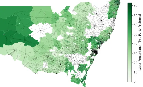
Census data is considered among the highest quality socio-economic data available. It is provided to the pub-lic via anonymised aggregated features whereby populations are grouped into geospatial areas according to the Australian Statistical Geography Standard - essentially tiling the nation into polygonal areas. The smallest of such areas for which the suite of Census socioeconomic data is available is the Statistical Area Level 1 (SA1) level, followed by a hierar-chy of successively larger regional aggregations (SA2, SA3 and so on). The SA1s are constructed as polygons using GIS ESRI shape files (provided by both the ABS and the AEC) which are two-dimensional maps geocoded according to a coordinate reference system. SA1 population counts vary between around 200 to 800 persons for most SA1s, with an average size of 400 persons (ABS 2016). GIS software was used to determine which SA1s neighboured each other from which a one-hop SA1 graph was constructed (see Fig-ure (1)). This process was repeated for the SA2 level (and SA3 level in one experiment). Links between SA1 and SA2-nodes were constructed using an ABS correspondence file connecting the levels.
Figure 1: Network of neighbouring regions constructed by finding polygon neighbours using GIS software. The edges connect the centroids of neighbouring regions. Colour in-dicates the two party preferred values used as the training signal. Some areas of the network span regions with missing data from the AEC source.
squares/robust line-fitting, MANOVA clustering and dis-criminant analysis. The experiments in this paper tested the efficacy of similar GLMs against standard and Hierarchical GCNN architectures.
Election data was sourced from the AEC, which pro-vides publicly available datapacks containing results from the 2016 election (AEC 2016). This includes electorate, SA1 and polling booth data available for download from their website. Our models were trained on the two-party preferred (2PP) vote which gives results give the results of ballots af-ter preferences have been distributed, usually between the Australian Labor Party and the Liberal/National Coalition. Adapting (Stimson and Shyy 2013), the 2PP results by booth were mapped onto the AEC’s publicly provided dataset de-tailing the number of voters from each SA1 at each respec-tive polling booth for the 2016 election, providing an esti-mate of 2PP at the SA1 level.
Hierarchical GCNN Much GIS data, especially Census data, falls within a natural hierarchical structure given by successively larger regional agglomerations. Hierarchical socio-economic GIS data can be decomposed into distinct heterogeneous graphs where lower-scale individual GIS fea-ture maps and graphs may differ from high-level regional or catchment-area data. A primary motivation of exploring the efficacy of GCNN models was the desire to capture the hier-archical nature of heterogeneous GIS networks. However, simply combining multi-level GIS graphs into one single large graph can become computationally intractable or lead to overfitting during model training and filter learning due to expanded parametrisation that comes from consolidation of adjacency matrices into an expanded adjacency relation. Therefore the capacity to run parallel GCNNs across net-worked but distinct graphs while controlling when to trans-mit information from one graph to another is important for GCNN GIS analysis. In this Hierarchical GCNN scenario,
the training and prediction is still made at the lowest level (SA1) of aggregation, but the higher level hierarchies pro-vide auxiliary information that is integrated using a residual connection near the end of the network.
Our starting point is to consider a two-level GIS hierar-chy comprising lower-level statistical areas (SA1s) (around 300 households each) and higher-level regional (suburban) statistical areas (SA2s) built from SA1 aggregations. Each level has its own graph generated via the GIS centroidal co-ordinates, with adjacency restricted to nearest-neighbours. For an SA1 graph ofn nodes and SA2 graph ofmnodes (m < n) we have an SA1 adjacency matrixA1 ∈ Rn×n and an SA2 adjacency matrixA2∈Rm×m. MatricesA3 ∈
Rn×mandA4 ∈ Rm×n are linear operators that facilitate information-sharing between the different-dimensional fea-ture spaces of each level. The embedding
A(3n×m):Rm×1→Rn×1, V(m×1)↦→V(n×1) (1) transfers information from the SA2 level graph to the SA1 level graph by acting on SA2 vertex vectorsV(m×1)(one for each SA1 feature), while the projection
A(4m×n):Rn×1→Rm×1, V(n×1)↦→V(m×1) (2) transfers information from the SA1 to SA2 level by acting on SA1 vertex vectorsV(n×1)(one for each SA2 feature). Here superscript terms in brackets indicate the dimension of the operator or vector. Filter-learning is conducted on both levels separately using a combination of graph convolution and graph pool embedding (Such et al. 2017) layers, with in-termittent projections and embeddings of features across the graph levels before combining to output ann-dimensional SA1-level output estimate for our predictor, 2PP vote by SA1.
Spatial domain convolutional filters for the SA1 and SA2 graphs are given by linear approximations to Cheby-shev polynomials (Such et al. 2017; Sandryhaila and Moura 2013)F = ∑k
i=0hkAk. Here the filterFis akth-degree polynomial of the graph adjacency matrixAkwhere the or-derkof each polynomial termAkencodes the number (k) of hops from a given vertex multiplied by the given filter tap (we setk= 1for simplicity). VerticesVare convolved with Fvia matrix multiplicationVout =FVin ∈Rn. Each hier-archical graph level’s convolution can then be approximated as:
F(1n×n)≈h1A (n×n)
1 F
(m×m) 2 ≈h2A
(m×m) 2 (3)
where there are several convolutional layers for each graph level, depending on the depth of the network. The hierarchi-cal model deploys parallel filter-learning at different graph levels with intermediate transfer of information between graphs using the learnt embedding operator filtersE=h3A3
and learnt projection operator filtersP=h4A4:
E(n×m)V(m×1)→V(n×1) (4)
P(m×n)V(n×1)→V(m×1) (5)
cvertex filter slices (one for each feature)F(1c)(the paren-theses index the specific feature) for the SA1 level anddlots ofm×mvertex filter slicesF(1d)for the SA2 level (in our case with only single adjacency matrix for each graph rather than multiple matrices for each edge feature as per (Such et al. 2017)). The choice of features for the SA2 level in ex-periments varied between a feature set identical to that of the SA1 nodes and smaller feature sets for different runs. There may be multiple (j) such filters bound up in a ten-sor form:F∈ Rn×n×c×j. The action of these operators on an input feature vector Vin(n×c) leads to in an output vec-torVout ∈ Rn×j (and analogously for the SA2 case). The feature tensor output forj filters for both the SA1 (withc
features) and SA2 (withdfeatures) levels is then:
V1(n,out×j)=(F1(n×n×c×j)V(inn×c))
n×j
+b(1n×j) (6)
V2(m,out×j)=(F2(m×m×d×j)V(inm×d))
m×j
+b(1m×j) (7)
with biasesbn×j (SA1) andbm×j (SA2). The final output prediction vector is at the SA1 level and is given byV(1n,out×1), obtained by further contractions.
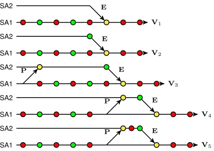
Hierarchical GCNN Variants To explore the effects of different layer-configurations and information-sharing across the SA1 and SA2 graphs, five variants (indicated by V1,. . .,V5) of Hierarchical GCNNs (shown in Figure (3)) were tested during the experiments. These are characterised by different arrangements of operations (either graph convo-lution layers shown by green nodes or zero-hop convoconvo-lutions shown by red nodes) and sequences of projection and em-bedding operations (yellow nodes). All networks were ini-tialised with two parallel graph channels. V1 architecture only included an embedding E(n×m) (indicated by a
yel-low node) from SA2 to SA1 feature space. This connection is a residual sum on each vertex vector, given by:
VSA(n×1)1 =E(n×m)VSA(m×1)2 W+V(SAn×1)1 ∈Rn (8) The best performance is found when no batch normalisa-tion and no activanormalisa-tion funcnormalisa-tion is performed after the addi-tion, which allows the smoothing of the direct path (He et al. 2016). The residual nature of the link means that information from the higher hierarchical layers are only incorporated if useful for the task, which is performed solely on the SA1 nodes.
V2 architecture was identical to V1 except for an addi-tional graph convolution layer (indicated by a green node) at the SA2 level. V3 architecture contained both a projection from the SA1 level to SA2 level, an additional graph con-volution layer with the first node with feature vector and a projectionP(m×n)from SA1 to SA2 feature space:
VSA(m×1)2 =P(m×n)VSA(n×1)1 W+V(SAm×1)2 ∈Rm (9) Variants V4 and V5 in Figure (3) incorporated additional projections and embeddings at later stages in the sequence.
Figure 2: Schema of SA1 and SA2 level graphs with links between them.
SA1 SA2
V1 E
SA1 SA2
V2 E
SA1 SA2
V3
P E
SA1 SA2
V4
P E
SA1 SA2
V5
P E
Figure 3: Hierarchical GCNN variants: green = graph con-volution; red = graph embedding; yellow = composition of SA1 and SA2 features (via projectionPor embeddingE).
Adaptive learning Despite being useful starting points, intrinsic GIS graphs may be sub-optimal for learning tasks. Because unsupervised learning of full optimal graph struc-ture from unstrucstruc-tured data is often intractable or complex (Hamilton, Ying, and Leskovec 2017), a ‘half-way’ point be-tween fully unsupervised graph learning and fixed adjacency is provided by semi-supervised adaptive graph learning in which input adjacency matrices are updated via a distance learning metric drawn from features related to the intrinsic GIS graph. Such methods have improved classification tasks and have been used in spectral convolutional settings.
In experiments below, we experimented with using a generic distance learning measure known within statistics as the generalised Mahalanobis metric (Li et al. 2018; Wang and Sun 2015; Perez, Ribeiro, and Perez 2016) nov-elly applying it in a spatial-filtering context. We used an
L2-norm with adjustable weights in which the distanceD
between two feature vectorsxi,xj ∈ Rc inc-dimensional features space is given as:
D(xi,xj) =
√
(xi−xj)TM(xi−xj) (10) where M is positive semi-definite precision matrix of weights of dimensionc2. Here indexiruns over the SA1
according to a GaussianG(xi,xj) = exp(D(xi,xj)/2σ2)
(assuming normalcy withσ= 1) using the Hadamard (ele-mentwise) product such that the embedding filter becomes:
G ◦En×m=h3G ◦A
3.
Experiments and Results
Methods Our experiments were designed to test the per-formance of the Hierarchical GCNN’s predictions of Labor 2PP by SA1 using Census features by comparison with a standard GCNN, multi-layer perceptron network (MLP) and the GLMs. Each experiment included both a standard super-vised training problem with five-fold cross validation (80%
training, 20%test) and two semi-supervised tasks with (i)
20%training,80%test and (ii)10%training,90%test. The full graph structure remains available despite the small size of the training set. The semi-supervised task is valuable as it is often desirable to extract information in the case where more training data is unavailable, such as observing overall patterns from a limited number of survey results.
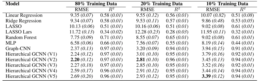
Centroid-to-centroid one-hop graphs for the SA1s and SA2s were constructed by finding polygon neighbours in open source QGIS software (Figure (2)). The resulting net-work for the whole state is shown in Figure (1). The GLMs chosen were: linear regression, ridge regression with cross-validation (CV), LASSO, LASSO Lars CV and Random Forest algorithms from Sci-Kit Learn. We also benchmarked against a densely-connected neural MLP (in which each SA1 as treated independently and not connected to any other) and the standard non-hierarchical GCNN (acting only on the SA1 graph). As the output is continuous, our primary metrics for comparison were RMSE and R2 for both the neural networks and GLMs.
A standard setting of two graph convolutional layers with 128 neurons for each except the last layer was used through-out the tests, although Fig 4 explores the performance un-der different settings for these hyperparameters. The ReLU activation function and the ADAM optimiser were used. Ta-ble (1) sets-out RMSE andR2 values (and standard
devi-ations) for each training/test split. One challenge when us-ing GIS data challenge is the ‘modifiable areal unit prob-lem’, namely whether zonal/aggregation or scale selection systematically biases aggregate results reliant upon statis-tics drawn from such aggregations (e.g. higher level geospa-tial aggregations). The Hierarchical GCNN model mitigates its potential impact by down-weighting the contribution of higher-level aggregated features if they do not contribute to model optimisation such that at worst the performance of the model will not decrease.
Discussion
GLMs and MLP As evident in Table (1), the benchmark GLMs performed significantly worse across all training/test partitions of the datasets by comparison with the standard GCNN and the Hierarchical GCNNs. The lower bounds RMSE for standard linear regression and ridge regression with CV were around9.35%with a maximumR2of0.58. In the10/90%semi-supervised case,R2and RMSE
deterio-rated. LASSO models performed worst, with RMSEs of just
Figure 4: RMSE of test set of standard GCNN vs Hierar-chical GCNN (V2) for one or two graph convolution (GC) layers and 64 or 128 neurons per layer
Figure 5: Absolute prediction error of Hierarchical GCNN subtracted from the absolute prediction error of the standard GCNN (difference clipped between 10 and -10). The geo-graphic spread shows that the Hierarchical GCNN clearly performs better (fewer brown areas in compared to blue), and seem to work especially well in regional areas.
above10%though interestingly they performed marginally better on the10/90%training/test split. The best performing GLM was the Random Forest with a RMSE around7.75%
andR2 of0.71. The basic MLP model outperformed each of the GLMs, achieving lower-bound RMSE of6.58%and
R2of0.66.
Table 1: Comparison of GCNN variants with traditional benchmarks, using RMSE andR2as measures. The five variants of the Hierarchical GCNN sequentially increase in complexity (standard deviations close to zero were rounded up to 0.01).
Model 80% Training Data 20% Training Data 10% Training Data
RMSE R2 RMSE R2 RMSE R2
Linear Regression 9.35 (0.07) 0.58 (0.01) 9.55 (0.12) 0.56 (0.01) 10.07 (0.82) 0.51 (0.08) Ridge Regression 9.34 (0.07) 0.58 (0.01) 9.53 (0.11) 0.57 (0.01) 9.86 (0.48) 0.53 (0.05)
LASSO 10.13 (0.06) 0.51 (0.01) 10.16 (0.06) 0.51 (0.01) 9.02 (0.08) 0.61 (0.01)
LASSO Lars 11.72 (0.13) 0.34 (0.02) 12.28 (0.23) 0.28 (0.03) 11.95 (0.11) 0.32 (0.01)
Random Forest 7.75 (0.09) 0.71 (0.01) 8.55 (0.07) 0.65 (0.01) 9.02 (0.08) 0.61 (0.01)
MLP 6.58(0.06) 0.66 (0.01) 7.56(0.07) 0.55 (0.01) 8.19(0.14) 0.44 (0.01)
Graph-CNN 2.37(0.13) 0.97 (0.01) 3.20(0.09) 0.94 (0.01) 3.94(0.15) 0.91 (0.01)
Hierarchical GCNN (V1) 2.24(0.12) 0.97 (0.01) 3.01(0.10) 0.95 (0.01) 3.79(0.16) 0.92 (0.01) Hierarchical GCNN (V2) 2.20(0.12) 0.97 (0.01) 2.81(0.10) 0.96 (0.01) 3.45(0.13) 0.94 (0.01) Hierarchical GCNN (V3) 2.27(0.18) 0.97 (0.01) 2.85(0.10) 0.95 (0.01) 3.52(0.16) 0.92 (0.01) Hierarchical GCNN (V4) 2.59(0.17) 0.96 (0.01) 2.91(0.12) 0.95 (0.01) 3.44(0.14) 0.94 (0.01) Hierarchical GCNN (V5) 2.69(0.20) 0.96 (0.01) 2.93(0.12) 0.95 (0.01) 3.39(0.12) 0.94 (0.01)
and of over75%by comparison with benchmark linear re-gression RMSE - representing a nearly three-fold improve-ment in RMSE and nearly two-fold improveimprove-ment inR2over the best GLM. For the semi-supervised cases, the standard GCNN also significantly outperformed all GLMs on both RMSE andR2.
Table (1) also demonstrates the improvement to the stan-dard GCNN architecture achieved via the novel introduc-tion of a hierarchical approach to GCNNs. The Hierarchical GCNN improved RMSE over the standard GCNN over both the supervised and semi-supervised tasks. The simple vari-ant V2 was able to decrease the RMSE to2.20%with 80% of the data in the training set and reduce RMSE to2.81%with 20% of the data in the training set. For both semi-supervised tasks, all variants outperformed the standard CNN on both RMSE andR2measures.
Figure (4) compares the performance over training epochs of the GCNN and Hierarchical GCNN for different neu-ron/layer number parametrisations. We can see that even with 80% of the data in the training set, the standard GCNN has a tendency to overfit with 64 neurons per layer. The test performance decreases as the number of epochs continues from 1000 to 5000. By comparison, we see that Hierarchi-cal GCNN achieves good performance with fewer epochs, is more stable and also has less performance variation between different number of layers and number of neurons.
By comparing the different variants of the Hierarchical GCNN, it can be seen that the specific structure of the Hier-archical GCNN impacts the performance depending on the nature of the task. Table (1) shows that a simple projec-tion operaprojec-tion with one graph convoluprojec-tion at the SA2 level works well in most cases and lead to the best performance when training on 80% of the data. Variations of additional complexity tend to increase training difficulty or increase overfitting in these circumstances. However for the small-est training/tsmall-est partition10/90%, increasing the number of operations at the SA2 level, including utilising an additional embedding operator led to the best performance. Variants V4 and V5 perform their embedding from SA1 to SA2 near the end of the network instead of the start, which allows the
em-bedded features to have undergone transformation and con-volutions within the SA1 branch.
In this case, the best performing Hierarchical GCNN V5 registered an RMSE of3.39%andR2of0.94, an decline in
RMSE of 0.55% and improvement inR2 of 0.03over the
standard GCNN. Having one graph convolution at the SA2 level seemed to always be beneficial compared to directly performing the projection operator filters. This suggests that the Hierarchical GCNN increases the receptive field of the SA1 nodes, with the residual link allowing only the useful information to be incorporated.
In all test/training partitions, the GCNNs outperformed even the best-performing GLM model. This is especially no-table when comparing the10/90%train/test split, in which both the standard GCNN (with RMSE of3.94%andR2 of
0.91) and Hierarchical GCNN (V5) (RMSE of3.39%and
R2of0.94) trained on10%of the data outperformed GLMs that were trained on80%of the data. Hierarchical GCNNs thus can outperform standard GLMs and a standard GCNN approach. Given the hierarchical and often sparse nature of socio-economic GIS training sets, the ability to utilise hier-archical graph structure to improve overall performance is potentially quite useful for researchers.
To understand the reason for the better performance of the Hierarchical GCNN, the maps in Fig. (5) visualise the difference in RMSE in the standard GCNN vs the Hierar-chical GCNN (averaged over the 10 repetitions of the semi-supervised task with 10% of the data in the training set). The Hierarchical GCNN outperforms the standard GCNN in many of the regional areas where the graph structure dif-fers substantially from the more geometrically regular city regions.
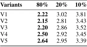
im-Table 2: RMSE of experiments using distance learning to adapt the weight of the projection edges. Bold indicates im-proved performance compared to the same variant in Table (1). Utility of these results was uncertain as standard devia-tions (suppressed) were in the order of 0.1%.
Variants 80% 20% 10%
V1 2.22 3.02 3.81
V2 2.15 2.81 3.43
V3 2.20 2.86 3.52
V4 2.50 2.92 3.45
V5 2.64 2.95 3.39
portant feature of its performance, providing an additional means by which information can be transmitted throughout the graph network between nodes not connected within their own graph level.
Table 3: RMSE of experiments including SA3 regions as an additional third hierarchy in the network. Bold indicates im-proved performance compared to the same variant in Table (1). Rows labelled ‘(with GC)’ include a graph convolution at the SA3 level
Variants 80% 20% 10%
V2 with SA3 2.52 2.97 3.60
V2 with SA3 (with GC) 2.29 2.77 3.37
V5 with SA3 2.66 2.90 3.28
V5 with SA3 (with GC) 2.66 2.90 3.35
The distance learning results for the Hierarchical GCNN variants were mixed and are presented in Table (2). All vari-ants with distance learning achieved lower five-fold RMSEs than the equivalent variants without distance learning for the supervised case. However, the variance in these results was similar in magnitude to any benefits gained, so the overall utility is uncertain. The addition of distance learning for the semi-supervised cases seemed to have little effect or slightly lower performance due to increased risk of overfitting.
Table (3) tests a further extension of the hierarchical ap-plication of our network, adding a third level (of SA3s) on top of the SA1s and SA2s. Doing so can produce further improvements, especially in the semi-supervised case as it further widens the receptive field of possible graph convo-lutions. Most models variants saw an improvement with the addition of the SA3 layer, including V5 on the 10%/90% dataset with an RMSE of 3.28%, making it the best per-forming of the sparsely-trained models. This again suggests the beneficial impact of incorporating auxiliary hierarchical graphs in the case of limited training data or sparse data sets. Although it wasn’t explored here, a key benefit of includ-ing networks at different aggregations is that it allows the use of data sources which are aggregated at different statistical levels (e.g. data sources from the tax office reported at the SA3 level). The projection and embedding operations de-scribed are general enough to allow the use of distinct node
features at each hierarchical level.
Conclusion and future work
The results of the experiments detailed in this paper demon-strate the utility of applying Hierarchical GCNN methods to GIS social-sciences problems, such as estimation of ag-gregate characteristics of populations within geographic lo-calities, and the improved performance of Hierarchical GC-NNs over standard GCGC-NNs, particularly in cases of mini-mal training data. As demonstrated via their high RMSE and comparatively lowR2 values, standard GLM methods
and MLP networks were not especially predictive of 2PP by SA1 on such GIS Census data.
The inclusion of both standard and Hierarchical GCNNs clearly has an effect, both in the fully supervised context (in which the majority of the data is used in the training set) and even moreso in semi-supervised contexts, precisely due to their capacity to leverage geographical connections. For Hierarchical GCNNs, the capacity to leverage multi-level geographic connections via higher-level graph convolutions while transmitting information between different graph lev-els appears to have played a role in its superior performance. In this paper, we have demonstrated the utility of GCNN methods for GIS in a social science context and the im-proved performance over standard GCNNs of novel Hierar-chical GCNN methods described above. HierarHierar-chical GC-NNs, which incorporate projections and embeddings be-tween different multi-level graphs, allow incorporation of multi-level socio-economic GIS data in a way that enriches the predictive insights from Census and other GIS datasets due in part to the Hierarchical GCNN’s capacity for incor-poration of neighbourhood features.
The significant performance improvement of Hierarchi-cal GCNNs over GLMs offers considerable potential for en-hancing modelling of voter behaviour along with the design and implementation of policy decisions across government industry, which often rely upon standard econometric tech-niques such as generalised equilibrium analysis to ascertain the impact of policy interventions on metrics, such as social welfare or GDP.
References
ABS. 2016. Census. Australian Bureau of Statistics. AEC. 2016. 2016 federal election results. Australian Elec-toral Commission.
Albert, A.; Kaur, J.; and Gonzalez, M. C. 2017. Using Con-volutional Networks and Satellite Imagery to Identify Pat-terns in Urban Environments at a Large Scale. In23rd ACM SIGKDD International Conference on Knowledge Discov-ery and Data Mining (KDD), Halifax, CANADA, Aug 13-17, 2017, 1357–1366.
Baker, E.; Bentley, R.; Lester, L.; and Beer, A. 2016. Hous-ing affordability and residential mobility as drivers of loca-tional inequality. Applied Geography72:65–75.
Bruna, J.; Zaremba, W.; Szlam, A.; and Lecun, Y. 2014. Spectral networks and locally connected networks on graphs. InInternational Conference on Learning Represen-tations (ICLR2014), CBLS, April 2014.
Defferrard, M.; Bresson, X.; and Vandergheynst, P. 2016. Convolutional Neural Networks on Graphs with Fast Local-ized Spectral Filtering.arXiv:1606.09375 [cs, stat]. Hamilton, W. L.; Ying, R.; and Leskovec, J. 2017. Rep-resentation Learning on Graphs: Methods and Applications. arXiv:1709.05584 [cs].
He, K.; Zhang, X.; Ren, S.; and Sun, J. 2016. Identity Map-pings in Deep Residual Networks. In Leibe, B.; Matas, J.; Sebe, N.; and Welling, M., eds.,Computer Vision – ECCV 2016, 630–645. Cham: Springer International Publishing. Henaff, M.; Bruna, J.; and LeCun, Y. 2015. Deep Convolutional Networks on Graph-Structured Data. arXiv:1506.05163 [cs].
Hewitson, B., and Crane, R. 2012. Neural Nets: Applica-tions in Geography. GeoJournal Library. Springer Nether-lands.
Heywood, I.; Cornelius, S.; and Carver, S. 2011. An In-troduction to Geographical Information Systems. Pearson Education Limited.
Jakeman, A.; Beck, M.; and McAleer, M. 1995. Modelling Change in Environmental Systems. Wiley.
Kipf, T. N., and Welling, M. 2016.
Semi-Supervised Classification with Graph Convolutional Net-works.arXiv:1609.02907 [cs, stat].
Li, R.; Wang, S.; Zhu, F.; and Huang, J. 2018. Adaptive Graph Convolutional Neural Networks. arXiv:1801.03226 [cs, stat].
Liao, E.; Shyy, T.-K.; and Stimson, R. J. 2009. Develop-ing a webbased eresearch facility for sociospatial analysis to investigate relationships between voting patterns and lo-cal population characteristics. Journal of Spatial Science 54(2):63–88.
Management Association, I. R., ed. 2013.Geographic Infor-mation Systems: Concepts, Methodologies, Tools, and Ap-plications. IGI Global.
Monti, F.; Otness, K.; and Bronstein, M. M. 2018. Mo-tifnet: a motif-based graph convolutional network for di-rected graphs.arXiv:1802.01572 [cs].
Noack, S.; Barth, A.; Irkhin, A.; Bennewitz, E.; and Schmidt, F. 2012. Spatial Modeling of Natural Phenomena and Events with Artificial Neural Networks and GIS. Inter-national Journal of Applied Geospatial Research (IJAGR) 3(1):1–20.
Nogueira, K.; Penatti, O. A. B.; and Santos, J. A. d. 2017. Towards Better Exploiting Convolutional Neural Networks for Remote Sensing Scene Classification. Pattern Recogni-tion61:539–556.
Openshaw, S., and Openshaw, C. 1997. Artificial intelli-gence in geography. Wiley.
Perez, J. L. R.; Ribeiro, B.; and Perez, C. M. 2016. Ma-halanobis distance metric learning algorithm for
instance-based data stream classification. In2016 International Joint Conference on Neural Networks (IJCNN), 1857–1862. Peters, R.; Schmitz, G.; and Cullmann, J. 2006. Flood rout-ing modellrout-ing with Artificial Neural Networks.Adv. Geosci. 9:131–136.
Polson, N. G., and Sokolov, V. O. 2017. Deep learning for short-term traffic flow prediction. Transportation Research Part C: Emerging Technologies79:117.
Sachdeva, S.; Bhatia, T.; and Verma, A. K. 2018. GIS-based evolutionary optimized Gradient Boosted Decision Trees for forest fire susceptibility mapping. Natural Haz-ards92(3):1399–1418.
Sandryhaila, A., and Moura, J. M. F. 2013. Discrete signal processing on graphs. IEEE Transactions on Signal Pro-cessing61(7):16441656.
Schram, A. 1992. Testing economic theories of voter be-haviour using micro-data. Applied Economics24(4):419– 428.
Seo, Y.; Defferrard, M.; Vandergheynst, P.; and Bresson, X. 2018. Structured sequence modeling with graph convolu-tional recurrent networks. In Cheng, L.; Leung, A. C. S.; and Ozawa, S., eds.,Neural Information Processing, 362– 373. Cham: Springer International Publishing.
Stimson, R., and Shyy, T.-K. 2013. And now for something different: modelling socio-political landscapes. The Annals of Regional Science50(2):623–643.
Such, F. P.; Sah, S.; Dominguez, M. A.; Pillai, S.; Zhang, C.; Michael, A.; Cahill, N. D.; and Ptucha, R. 2017. Ro-bust Spatial Filtering With Graph Convolutional Neural Net-works.IEEE Journal of Selected Topics in Signal Processing 11(6):884–896.