Measuring, Understanding, and Estimating the Influence of the Environment on low-power Wireless Networks

(1)

PhD Dissertation

International Doctorate School in Information and Communication Technologies

DISI - University of Trento

Measuring, Understanding, and Estimating

the Influence of the Environment

on Low-Power Wireless Networks

Ramona Marfievici

Advisor:

Prof. Gian Pietro Picco

Universit`a degli Studi di Trento

Co-Advisor:

Dr. Amy Lynn Murphy

Fondazione Bruno Kessler, Trento

(2)

(3)

(4)

(5)

“Be good!”

(6)

(7)

The following document, written under the supervision of Prof. Gian Pietro Picco and Dr. Amy L. Murphy, was reviewed by:

Prof. M´ario Alves Polit´ecnico do Porto, Portugal

Prof. Alberto Cerpa University of California, Merced, USA

(8)

(9)

Abstract

After a decade and a half of research in academia and industry, wireless sensor networks (WSNs) are seen as a key infrastructure able to monitor the environment in which they are immersed, thanks to their miniaturization, autonomy, and flexibility. Still, outdoor deployments of WSNs (e.g., in forests) are notoriously difficult to get right, partly due to the fact that their low-power wireless communication is greatly affected by the character-istics of the target environment (e.g., temperature, humidity, foliage). In the absence of quantitative evidence about the target application environments, the asset that drives a successful and reliable outdoor deployment is the experience gained from previous deploy-ments, lab-like testbeds, or simulators that however often do not resemble the real-world environments.

The general goal of this dissertation is tosupport the principled design and deployment of WSNs by improving the understanding of how the natural outdoor environment affects the network stack, and providing tools and modeling techniques to address this impact. This constitutes the premise for WSNs to be a credible tool for domain experts (e.g., biologists) operating in this field. Our own practical need to design and deploy a reliable WSN system for wildlife monitoring in the mountains near Trento, Italy, pushed our goals towards a deployment and application oriented perspective, whose ultimate objectives are: supporting the WSN deployment; informing the selection or design of protocols, to ensure they are well-suited to the target environment; deriving models to push the envelope of what can be predicted or simulated beforehand.

To achieve these goals we must start from the first step—assessing quantitatively the characteristics of the low-power wireless links in-field, i.e., in the environment where the WSN must be deployed. To this end, we contribute with Trident and Harpoon,

(10)

We argue that the tools we expressly designed for gathering in-field empirical traces, the understanding and quantitative characterization of data traces from real environments, and the modeling, together significantly advance the state of the art by rendering the process of designing and deploying a WSN more repeatable and predictable.

Keywords

(11)

List of Tables

3.1 Trident per-round configuration parameters. . . 24

3.2 In-field commands. . . 25

3.3 Platform support in Trident. . . 27

3.4 _Harpoon per-round configuration parameters. . . 31

4.1 Campaigns. . . 37

4.2 Values for per-round configuration parameters for phy experiments using the cross. . . 41

4.3 Percentage of asymmetric links on cross . . . 52

4.4 Transitions on _cross . . . 53

4.5 Values for per-round configuration parameters for _phy experiments using the grid. . . 54

4.6 Asymmetrics links on grid . . . 60

4.7 Transitions on grid. . . 60

4.8 Per-round configuration parameters and their values for grid topology campaigns. . . 61

4.9 Delivery rate statistics . . . 68

4.10 Duty cycle statistics . . . 68

4.11 Retransmissions count statistics . . . 68

4.12 ORW L2 duplicates . . . 72

5.1 RSSI-temperature linear function slopes on _grid. . . 78

5.2 LQI-temperature linear function slopes on summer grid. . . 81

5.3 Our proposed model. . . 88

5.4 Boano et. al [18] model. . . 88

5.5 Day vs. night PDR distributions example. . . 89

5.6 Comparison between empirical traces and simulated traces: overall PDR (%). . . 94

(16)

5.8 Comparison between empirical and simulated traces: summer and winter night link classification. . . 95 5.9 Comparison between empirical traces and simulated traces: number of

(17)

List of Figures

1.1 Dissertation Contributions. . . 4

2.1 Connected, transitional and disconnected region example. . . 10

3.1 SampleTridentexperiment showing two rounds, staggered transmissions using single-packet and burst probes, and per-round synchronization. . . . 22

3.2 The Trident toolset. . . 25

3.3 The “results view” of the Trident in-field assistant, showing one-hop inbound connectivity and PDR for node 0. . . 26

3.4 ZigBee transmits each broadcast packet three times. . . 29

3.5 Distribution of packet arrival time. . . 29

3.6 The Harpoon toolset. . . 32

4.1 Experimental sites on Mount Bondone. . . 38

4.2 WSN nodes in the field. . . 39

4.3 Network topologies for experiments. . . 39

4.4 Distribution of link distances. . . 40

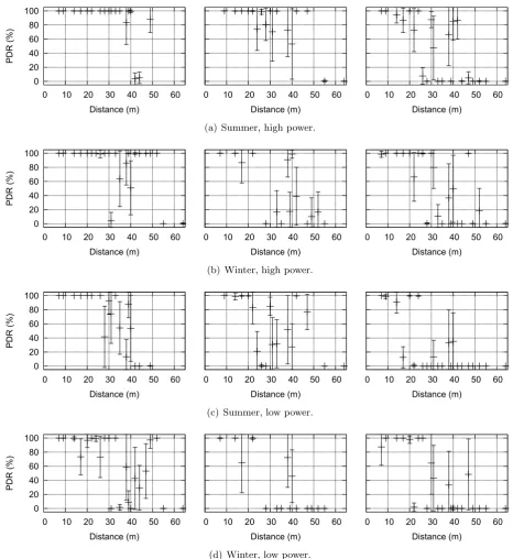
4.5 Network-wide average PDR, for all combinations of site (open, spruce, beech), season (summer vs. winter) and power (high vs. low). . . 41

4.6 Transitional areas in open (left), spruce (center), and beech (right). . . 43

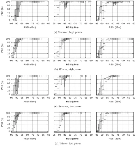
4.7 RSSI vs. PDR inopen (left), spruce (center), and beech(right). . . 45

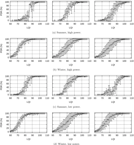
4.8 LQI vs. PDR inopen (left), spruce (center), and beech(right). . . 46

4.9 Link classification. . . 47

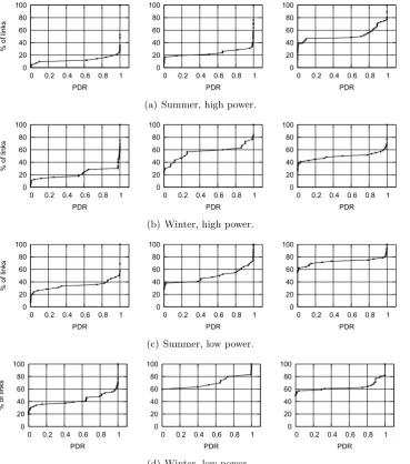
4.10 Cumulative distribution function ofPDR in_open (left),_spruce (center), and beech (right). . . 47

4.11 Seasonal variations, at high power (left) and low power (right). . . 48

4.12 An example of day vs. night variations: the PDR of link 2→6 and 6→2 in open, during summer, at low power. The node distance is 39 m. . . 49

4.13 Day vs. night variations, at high power (left) and low power (right). . . 51

(18)

topologies. . . 55

4.15 Network-wide average PDR in winter: comparison of the experiments in Section 4.2.2 and 4.2.9, performed one year apart and with different topolo-gies. . . 56

4.16 Meteorological conditions: temperature and humidity (left) and precipita-tion (right). . . 56

4.17 Daily variations in_open, at high and low power. The sudden drop to zero corresponds to the 1-hour period in which, every two days, we downloaded the data from the flash of the nodes, and replaced their batteries. . . 57

4.18 Winter link classification, at high power (left) and low power (right). . . . 58

4.19 Day vs night variations, at high power (left) and low power (right). . . 59

4.20 Delivery ratio forCTP in open (left) andspruce (right) during summer. 63 4.21 CTP beacons inopenandspruce, high (left) and low (right) power during summer. . . 63

4.22 Parent changes in_open and _spruce, at high power during summer. . . 63

4.23 Delivery ratio for CTP in _open (left) and _spruce (right) during winter. . 65

4.24 CTP beacons inopenandspruce, high (left) and low (right) power during winter. . . 65

4.25 Delivery ratio for CTP on grid (4th campaign) and grid small (6th campaign). . . 67

4.26 CTP and ORW delivery ratio on grid small. . . 67

4.27 Delivery ratio forCTP and ORW. . . 69

4.28 Environmental conditions during the experiments. . . 69

4.29 CTP ACK fails and lost packets variations with temperature, at node 5 (left) and node 6 (right). . . 70

4.30 CTP ACK fails and lost packets variations with humidity, at node 5 (left) and node 6 (right). . . 70

4.31 Duty cycle ofCTP and ORW. . . 71

4.32 Retransmissions of CTP and ORW. . . 71

4.33 The effect of environment on contact detection. . . 73

5.1 RSSI and temperature relation. . . 78

5.2 RSSI and PDR of TMote Sky and Waspmote links over a 2-day time period. 79 5.3 TMote Sky RSSI-temperature relation in sauna. . . 80

5.4 Waspmote RSSI-temperature relation in sauna. . . 81

(19)

(20)

(21)

Chapter 1

Introduction

“Begin at the beginning”, the king said, very gravely,

“and go on till you come to the end: then stop.”

Lewis Carroll,Alice in Wonderland

In 1999, researchers working on “Smart Dust” [37] pioneered the concepts of a large number of resource scarce devices cooperating to achieve a sensing task. Since then, a whole range of algorithms, protocols and programming abstractions have been developed for these wireless sensor networks (WSNs), along with several operating systems and hardware platforms. Moreover, the validity and the performance of the proposed solu-tions has been extensively tested in laboratories, in simulators and controlled testbeds. To a large part driven by the functionality and performance demonstrated in research laboratories, WSNs are nowadays seen as flexible systems able to provide dense and cost-effective monitoring for application domains that span engineering, scientific, medical and other disciplines. This has created, from the domain experts, enormous expectations around this technology, as an enabler of previously impossible scenarios as well as credible replacement for established solutions.

Motivation. Since the inception of WSNs, many target applications meant that the network would be deployed in outdoor settings, where temperature, humidity, foliage, obstacles and other factors are known to affect communication especially in the 2.4 GHz ISM band [1] that has become a popular choice among researchers and practitioners. In fact, examples of successful deployments covering a wide range of scenarios from envi-ronmental monitoring [9, 10, 54, 65, 74, 83], to habitat monitoring [25, 49, 56, 73], from precision agriculture [43] to the study of tree canopy climate [48, 77] exist. However, these experiences also clearly demonstrate: (i) how difficult it is to run and manage a WSN in the real-world rather than in an indoor controlled testbed, (ii) that all too often these systems fail to provide the expected results once deployed in theiroutdoor target

(22)

ments. This is partly due to the fact that the behavior of their physical communication layer and, as a consequence, of the entire stack, is greatly affected by the characteristics of the environment. However, the lack of proper tools for large-scale, in-field connectiv-ity assessment, and consequently of publicly available traces means that there is limited quantitative evidence for understanding channel behavior in the target environment.

This lack of understanding prevents the development of channel models realistic enough to capture the characteristics of the target application environments, which in turn are needed to predict and estimate link quality at run-time, or reproduce network condi-tions accurately when simulating the application behavior. As a result, WSN design and deployment is still mostly an art, based on rules-of-thumb guidelines gleaned from experi-ence, or lab-like testbeds which have little in common with the real target environments, especially when these are outdoor.

A concrete application. In this dissertation, we are motivated by a real-world wildlife monitoring application and WSN deployment [56] we are pursuing in collaboration with biologists studying the social interactions/contacts among animals, namely, roe deer in the mountains near Trento, Italy.

(23)

3

Goals and contributions. The general goal of this dissertation is to

support the principled design and deployment of WSNs by improving the un-derstanding of how the natural outdoor environment affects the network stack, and providing tools and modeling techniques to address this impact.

This constitutes the premise for WSNs to be a credible tool for domain experts (e.g., biologists) in outdoor environments. For this it is necessary to understand and characterize quantitatively and empirically the behavior of the WSN in the target environment.

Today, tools enabling the collection of network connectivity measurements in out-door real-world environments are lacking. Therefore, large realistic network connectivity datasets are missing in the literature, further limiting the understanding of the behavior of low-power wireless links and the development of realistic models able to predict (e.g., for protocol design) or to reproduce (e.g., for simulation) the behavior of the network links. Moreover, the lack of quantitative evidence about target environments leaves the WSN developers in the dark, without specific guidelines to drive their deployments and tune their systems and protocols.

The main contributions of this dissertation, as depicted in Figure 1.1, can be summa-rized as:

1. atoolsetfor in-field connectivity and routing protocol performance assessment that supports principled, repeatable, automated and flexible collection of measurements in the target environment, relies only on the WSN nodes without any external in-frastructure, and does not require any coding by the end user;

2. the analysis of a large set of data traces collected in vivo (i.e., in actual real-world environments) in which we quantify the impact of the environmental factors, both in terms of morphology (e.g., vegetation present), as well as daily, seasonal and yearly variations at the physical, routing and application layer;

3. models based on these traces, with the distinctive goal to:

(a) describing the influence of temperature and humidity on low-power wireless links for estimating link quality at run-time;

(b) describing thelong-termbehavior of low-power wireless links collected in-field for reproducing realistic network conditions in simulators.

(24)

Figure 1.1: Dissertation Contributions.

an infrastructure made by powered devices to which the motes are wired for gathering ex-perimental data — a luxury one can rarely afford in-field. Therefore, the first contribution of this dissertation is embodied in twotools,TridentandHarpoon, expressly designed to support principled, repeatable, automated and flexible collection of connectivity mea-surements and routing protocol performance assessment in the target environment. Unlike similar tools, _Trident and _Harpoon do not require any communication infrastructure besides the WSN nodes. Our tools cover the entire process concerned with in-field connec-tivity and routing protocol performance assessment, from the design of the experiments to the download and analysis of the data gathered. Our tools are designed to be easy to use by domain experts (e.g., the biologists we collaborate with) who can perform their experiments without any coding effort. Trident is provided in two variants, targeting TMote Sky motes running TinyOS, and Waspmotes running the standard ZigBee stack, covering popular platforms in research and industry, respectively. The tool supports the acquisition of physical layer parameters (e.g., PDR,RSSI,LQI, noise floor), while Har-poon supports the acquisition of routing layer metrics (e.g., data yield and duty-cycle), which account for the reliability of communication, along with the overhead and energy consumption necessary to ensure this reliability in the target environment. Harpoon supports two routing protocols: the Collection Tree Protocol (CTP), a representative of commonly employed tree-based routing schemes, and the Opportunistic Routing Pro-tocol (ORW), a more recent protocol based on opportunistic routing approach. If the protocol allows, Harpoon acquires additional parameters to assess the effectiveness of specific mechanisms (e.g., number of beacons for CTP, number of neighbors for ORW). Both tools support the acquisition of environmental parameters (e.g., temperature and humidity) from on-board sensors.

(25)

5

experimental sites are on Mount Bondone, near Trento, Italy. In collaboration with the biologists in our team, we identified three characteristic locations in this area: a meadow with essentially no trees (open), an evergreen forest with sparse vegetation (spruce), and a deciduous forest with dense vegetation (beech). The design of the experiments was informed by the biologists interest in understanding how low-power wireless links and as a consequence the contact detection are affected by: presence and density of vegetation,

seasonal anddaily variations. Our experiments investigated, during six campaigns, across multiple years, what happens if thesame WSN is immersed in different combinations of the above environmental factors. We quantify the trends emerging at the physical layer and show that: (i) this influence is mirrored at the routing and application layer, (ii) the macro-trends across environments allow us to infer the relative trends in reliability, overhead and energy consumption at the routing layer.

Whilst there are other empirical studies showing that the physical layer is affected by the environment, our study extends up to the routing layer, which bears a direct impact on the application performance. To the best of our knowledge, this represents the first empirical study that characterizes, from a quantitative standpoint, the overall behavior of a WSN in different environments.

As a third contribution, we build on the above analysis to exploit the set of data traces to create two models: (i) for estimating the link quality and run-time, and (ii) forreproducing realistic network conditions in simulators.

First, based on our empirical observations that the link quality of a WSN depends on the characteristics of the surrounding environment, we focus on two factors: temperature and humidity. We study the impact of these two factors on the physical layer parameters in the open field environment as the degradation of the link quality here is not influenced by any other environmental factors (e.g., obstacles, foliage). We conducted a study on the impact of temperature on theRSSI andPDR of two hardware platforms, TMote Sky and Waspmote, and show that the latter is affected by temperature to a much lesser extent w.r.t. the former. Then, we develop a model describing the influence of temperature and humidity on the link quality. This helps estimating the link quality at run-time considering the particular temperature/humidity profile of the target environment and informing the application layer performance.

(26)

(27)

Chapter 2

Background and Related Work

What’s past is prologue.

William Shakespeare,The Tempest

This chapter presents background on experiences from outdoor real-world WSNs de-ployments and their related challenges. Software tools developed to measure and analyze low-power wireless links along with systematic empirical studies on low-power wireless transmissions are reviewed. Finally, existing models characterizing the behavior of low-power wireless links are presented.

2.1

Long-lived Real-World Deployments

Taking a closer look at prior long-lived real-world deployments reveals that putting a functional WSN in place is a non-trivial task. Several research groups have already shared part of their experience in the WSNs deployment field, e.g., X-sense [9], Permadaq [10], Koala [54], Luster [65], WildScope [56], LOFAR-agro [43], GreenOrbs [48], WildScope [56], Great Duck Island [73], Permasense [74], Redwoods [77]. The lessons learned from these deployments highlight a tremendous gap between “it works in the lab” and “it works in the real-world” [81]. They also emphasize the need to understand the target environment and the impact it will have on the operation of the WSN, as well as the need to take into account the domain knowledge and application requirements to enable successful long-term outdoor deployments. Moreover, they advocate for the need of deployment-time tools to guide the deployment, support in-field evaluation of alternatives and ensure the deployment is up and running before leaving the field. Moreover, there are several examples, TASK [15], Sensorscope [63], Heathland [79], Vigilnet [80], Marionette [84], where a protocol developed on a testbed does not work well in the actual deployment.

(28)

However, all these real-world reported experiences focus on the WSN performance in terms of high-level network properties such as end-to-end throughput, data yield and latency and a characterization of the low-power wireless links and routing protocol per-formance in these scenarios is largely missing. Moreover, the reports that complemented these deployments do not aim to characterize the environment where they are deployed and its variations.

2.2

Tools for In-Field Measurements

The WSN community has recognized the relevance of acquiring information about the properties of the wireless links in the specific environment and built tools to empirically experiment with links. SCALE [20], SWAT [70], RadiaLE [5], and IRIS [28] were conceived for this.

SCALE is built using the EmStar programming model [31] and collects only PDR. Each node runs a software stack, allowing for sending and receiving probe packets in round-robin, retrieving packet-statistics and sending them through serial communication. All nodes are connected to a central PC via serial cables and multiplexors. The PC runs different processes, one for each node in the experiment, that perform data collection. Based on the collected data, other processes running on the PC allow for connectivity assessment through the computation of the PDR for each unidirectional link. Thus, the network connectivity can be visualized at run-time.

SWAT collects PDR and hardware-based metrics, i.e., RSSI, LQI, noise floor. It uses the same type of infrastructure as SCALE, nodes being connected through serial connections or using a back-channel to a central PC. SWAT stores collected data into a database and provides modules for calculating and visualizing various metrics derived from statistics.

RadiaLE makes use of bursty and synchronized traffic patterns for physical layer mea-surements collection. Nodes are connected to a control station via a combination of USB cables and active USB hubs constituting a USB tree. This tree is used as a reliable logging/control channel between the nodes and the central PC. RadiaLE supports the operator to follow the experiment progress in real-time by displaying the network map, link quality metrics and node status. Moreover, it logs the measurements in a database and enables the evaluation of Link Quality Estimators (LQEs) that can be configured and evaluated based on the collected data from a given experiment.

(29)

2.3. EMPIRICAL STUDIES 9

On the other hand, IRIS provides an integrated solution for experiment management and on site data analysis. It supports the automated experiment installation on nodes, the management of measurements, i.e., data organization and logging in different formats (binary, CSV or WiseML format [2]), and customized logging with the help of user-defined functions for direct manipulation of raw data. Furthermore, the tool allows to control the experiment flow and the interaction with the deployed WSN. IRIS is equipped with a set of function templates for data processing and interfaces for visualizing the experiment data.

Unfortunately, IRIS does not support the configuration of the experiment and neither generates the code for the experiments, thus the user has to get into code intricacies and provide the code to be run by IRIS.

In Chapter 3, we present Trident and Harpoon, our tools expressly designed to simplify the chore of in-field connectivity and routing protocol performance assessment. These tools rely only on the WSN nodes whose connectivity needs to be ascertained, without any external infrastructure. They cover the entire workflow concerned with the experiments which can be configured easily without requiring any coding.

2.3

Empirical Studies

The performance of a WSN deployment is obviously directly affected by the quality of the links enabling the communication among nodes. In the case of commonly-used IEEE 802.15.4 radios, the link quality is in turn easily affected, as empirically demonstrated, by environmental factors (i.e, temperature, humidity, rainfall, snow, wind, foliage, ob-stacles), which cause variations over time and space. Therefore, from a communication perspective, information about the properties of the low-power wireless links in the specific environment at hand is crucial to build reliable systems that run on top of 802.15.4.

2.3.1 Metrics

Researchers have identified several low-level metrics to help them understand network dynamics. The set of basic metrics that were examined by previous empirical studies to capture the low-power link characteristics are: PDR (Packet Delivery Ratio), RSSI

(30)

gray area

Figure 2.1: Connected, transitional and disconnected region example.

measures the RF signal strength of a received packet. Noise floor is the power of the ambient channel energy, when there are no transmissions, and is useful to indirectly determine the presence of interference. SNR of a received packet is computed as the difference between the two RSSI measures (i.e, RSSI and noise floor). LQI is computed over the 8 bits following the start frame delimiter (SFD) and for the CC2420 radio ranges from 50 (minimum) to 110 (maximum).

2.3.2 Empirical Studies on Link Properties

A significant body of works is related to the understanding of link dynamics, showing how their quality fluctuates over time [22, 69, 87] and space [20, 29, 61, 86, 87, 88, 91], that connectivity is typically asymmetric due to differences in noise floor [22, 88] and to imperfections in hardware [91] that may cause variations in the power output during transmissions, and/or antenna orientation [61, 88].

These works demonstrated that the transmission range is not isotropic and is defined by three regions- connected, transitional, and disconnected, based on the distance of the receiver from sender and on the PDR, as shown in Figure 2.1. The connected region is the closest to the sender and its links are of good quality. At the other extreme, the disconnected region is the farthest from the sender,: it does not contain links usable for communication. The transitional region, also called the “gray area” is a mix of the two, and contains links that exhibit a high variance. Each of these regions has an irregular shape, with bounds changing over time and with specific features [20, 61, 87, 90].

(31)

2.3. EMPIRICAL STUDIES 11

measurements using Mica1/Mica2 platforms and different power levels and reported the width of transitional region to range from 50% to 80% of the transmission range. On the other hand, Zhao and Govindan [87], while performing measurements with almost the same settings as of Cerpa et al. [20], reported a smaller width for the transitional region ranging from 20% to 35% and a range for the percentage of intermediate links from 35% to 50%. Moreover, Srinivasan et al. [69] claimed that the number of intermediate links observed with recent platforms, Micaz and TelosB, is lower, from 5% to 60%, than that observed with old platforms. Mottola et al. [53] refuted this observation while conducting experiments in road tunnels using TMoteSky platform. Nevertheless, these studies are based on different network settings in terms of radio type, power, environment and traffic load but all showed that link quality varies drastically over space.

Studies show that the temporal variations of link quality are due to changes in the environment, constructive/destructive interference, obstacles and human presence [21, 87, 61, 75]. Cerpa et al. [21] and Zhao and Govindan [87] show that links from disconnected and connected regions tend to be stable over time, while Srinivasan et al. [69] report on link burstiness and confirme observations made by Cerpa et. al [22].

Moreover, Cerpa et al. [20, 21] analyzed the asymmetry of low-power links and showed that links from transitional region tend to be asymmetric and argued that link asymmetry is not correlated with distance. Srinivasan et al. [69] studied the temporal variation of link asymmetry and found that very few links are long-term asymmetric. Experiments of Mottola et. al [53] refuted this and show that link asymmetry tends to persist in their specific environment.

With few exceptions [20, 53, 69], the above studies were carried out indoor, in con-trolled environments and present radically different (and sometimes contradicting) results. In contrast, our experiments presented in Chapter 4, are carried out in-field and outdoor. Moreover, these works are generally focused on the study of individual links, usually over short-term variations, to provide guidelines on fine-grained design decisions. In contrast, we are concerned with characterizing the aggregate behavior of the network. In doing this, however, we do borrow some commonly-used concepts, definitions, and techniques from these works, e.g., including the notion of transitional area, the definition of link classes and asymmetric links.

2.3.3 Impact of the Environment on Low-Power Wireless Networks

(32)

site. Works of Anastasi et al. [4] and Son et al. [67] suggest that fog and rain may have a severe impact on the transmission range of WSN nodes, especially w.r.t. packet reception. A loss of connectivity in their outdoor deployments, with rainfalls from 0.4 to 1.4 mm and temperature daily variations between 10 and 50◦C, was reported by Sun and Cardell-Oliver [72]. Similarly, Capsuto et al. [17] reports a drop in signal strength during rain and snowfall.

Work by Holland et al. [36] concludes that temperature and humidity have no impact on link quality and data yield while Bannister et al. [7] show that high temperature negatively affects communication, based on data from a radio survey in the desert and applied to simulations of localization and data collection. Daily variations in RSSI of up to 6 dBm were reported by Lin et al. [47]. In particular, Boano et al. [13] quantified the impact of these conditions on different platforms in an outdoor industrial setting, showing that light rainfall has a negligible effect on signal strength while heavy rainfall can disrupt connectivity. Using a controlled experiment, Boano et al. [12] show a decrease in RSSI as temperature increases and reasons that changes in temperature affect crystal accuracy that induce frequency shifts, and thermal transceiver noise, that may degrade performance. More recent work of Wennerstr¨om et al. [82] reports a clear degradation in PDR and average link quality during summer and confirm that daily fluctuations of ambient temperature have a strong impact on quality of the communication. Motivated by this study, Boano et al. [18] carry out a systematic set of experiments in controlled settings analyzing how temperature affects the RSSI in transmitters and receivers of nodes with CC2420 and CC2520 radios and show that the trend can be captured in a simple first-order model. Schmidt et al. [64] built “HotBox” and reproduced the setup from [18]. They reinforced that temperature has a significant influence on communication quality but reported that heating the receiver produces a larger impact on link quality rather than heating the sender as Boano et al. [18] showed.

Temporal relationship between RSSI variability and plant canopy development is ob-served by Rankine et al. [59] in an old growth stand of deciduous forest. In an effort to understand the causes of losses in a forest deployment, Dong et al. [24] observes periodic performance variations with links severely degrading during night and recovering during day. Moreoever, wind movement through vegetation has been observed to increase the variance ofRSSI due to the changes in multi-path propagation as trees sway in the winds. Hashim and Stavrou [35] show that high wind speeds produces radio signal fading of the 2.4 GHz radio frequency.

(33)

2.3. EMPIRICAL STUDIES 13

protocols and the application when operating a WSN outdoors.

Using the same GreenOrbs deployment as [24], Tong et al. [78] makes one step further and looks at the routing dynamics analyzing possible causes ofCTP parent change events during several days and their correlation across time and location. Keppitiyagama et al. [40], investigates the effect of temperature fluctuations on RPL protocol [85], in a temperature-controlled testbed, and shows that the performance of ContikiRPL suffers from the short term validity of the ETX [23] predictions under temperature fluctuations. In Chapter 4 we confirm many of the above mentioned findings. However, in compar-ison, our work assesses the overall trends induced by the environment in a more holistic way, by taking into account yearly, seasonal and daily variations. It also explores the effect of environments with different characteristics (e.g., vegetation). Finnaly, we extend up to the routing layer, which bears a more direct impact on the application performance, and the application layer, the one directly relevant to the end user. Moreover, we investigate if the observed influence of the environment at the physical layer is mirrored at the upper layers.

2.3.4 Empirical Studies on Data Collection Protocols

Several studies evaluate the performance of data collection protocols [27, 30, 32, 51, 58] and benchmark the proposed solutions against CTP. Gnawali et al. [32] reports CTP’s

data yield ranges from 90.5% to 99.9%, a median duty-cycle of 3% across the nodes of a network in experiments in which the network generates data at 30 packets/minute and delivers them to the sink.

The performance of ORW protocol was evaluated by Ghadimi et al. [30] in both simulations and testbed-based experiments. They show that ORW improves duty-cycle

and delays significantly while achieving similar reliability and transmission counts when compared to CTP. An average decrease in duty-cycle by about 50% and up to 90% for individual nodes is reported along with a decrease in delay by 30% to 90% depending on the network density. Moreover, they show that the optimal ORW duty-cycle is at lower wakeup rates when compared to CTP. At high wakeup rates ORW loses some of its benefits and both protocols show similar performance in terms of energy and delay.

The testbed evaluation in Puccinelli et al. [58], where Broadcast-free Collection Pro-tocol is benchmarked againstCTP, shows a reduction of theduty-cycle of the same order of the one achieved byORW.

When compared the Backpressure Collection Protocol [51] againstCTP on a 40-nodes testbed, a performance by more than 60% in terms of min-max rate and a reduction by more than 30% in terms of average packet transmissions was observed.

(34)

done in simulations and testbeds. The only exception, represented by Gnawali et al. [32], evaluates CTP’s performance on a large-scale, long-term deployment, using CTP in an application that collects power and utilization data for the computing infrastructure of a building. In contrast, our experiments are carried outdoor. Not only that we investigate the performance of the data collection protocols but also assess the effectiveness of their specific mechanisms. Moreover, throughout our study we investigate and evaluate the coupling between subtle effects at the physical layer and routing layer behavior.

2.4

Models for Characterizing the Behavior of Low-Power

Wire-less Links

Several models cover outdoor and indoor signal propagation characterization, taking into account the number, delay and power of indoor multipath components. The log-normal path loss model [60] has been widely use to describe the propagation of radio signals for low-power wireless networks and small-scale models that estimate signal loss over small distances and small time intervals [55] have been proposed as well.

Another class of models, on the other hand, estimate the packet delivery function. These models build functions relating physical layer parameters (e.g., RSSI, SNR) to

PDR. The delivery probability is modeled as a function of interference by Reis et al. [62], while Kashyap et al. [39] uses curve-fitting of packet reception probability and SNR

to model the packet reception. Woo et al. [86] derives a packet loss model based on aggregated statistical measures, assuming a Gaussian distribution of PDR for a given transmitter-receiver distance, which later was refuted by Zuniga and Krishnamachari [91]. They use the log-normal path loss model to derive expressions for the distribution, expec-tation, and variance of PDR as a function of distance. A set of non-parametric statistical models for characterizing links and groups of links associated with a particular receiver, transmitter, radio is developed by Cerpa et. al [21].

Recent efforts provide models for estimating the signal strength as a function of tem-perature. Bannister et al. [7] quantifies the loss ofRSSI due to temperature for Telos-class nodes, but only for a limited temperature range (i.e., 24 to 65◦C) and for a single radio chip. Using TempLab [11] testbed infrastructure, Boano et al. [18] captures the impact of the temperature on the signal strength of transmitters and receivers of two radio chips, i.e., CC2420 and CC2520, and show that the decrease in RSSI is consistent among different platforms. Then, a first order platform model describing the impact of the temperature on wireless sensor nodes is proposed. Nevertheless, TempLab temperature profiles are over 0◦C, covering just a segment of the outdoor temperature profiles.

(35)

2.4. MODELS FOR CHARACTERIZING THE BEHAVIOR OF LOW-POWER

WIRELESS LINKS 15

a wide chasm between real-world channel behavior and existing radio channel models in simulators [38]. The latter are often too simplistic, and can hardly capture the complex-ity of the real-world. To increase the realism of simulations, several models have been proposed and incorporated into existing simulators. Using a multi level approach involv-ing hidden Markov models and mixtures of multivariate Bernoullis, Kamthe et al. [38] proposed to model the long- and short-term scale behavior of links. Zuniga and Krishna-machari [91] modeled the behavior of wireless links depending on the radio and channel characteristics for static and low-dynamic environments, while Lee et al. [45] proposed a statistical model created from noise traces. On the other hand, instead of attempting to create more precise and realistic radio models for simulators, Boano et al. [14] proposed to augment existing simulation tools with the playback of realistic interference traces.

(36)

(37)

Chapter 3

Measuring: Tools

Door meten tot weten.

By measurement to knowledge.

Heike Kamerlingh Onnes

Real-world deployments of WSNs are notoriously difficult to get right, partly due to the fact that their low-power wireless communication is greatly affected by the character-istics of the target environment. Communication in the 2.4 GHz ISM band has peculiar characteristics, that have been studied by many researchers; a summary is provided in Section 2.3.

Unfortunately, the tools supporting connectivity assessment [5, 20, 70] were conceived to study the properties of low-power wireless links using an infrastructure made by pow-ered devices to which the motes are wired, and thus are not directly applicable in most deployed systems where nodes are only wirelessly connected. Further, they are of limited use for characterizing any outdoor environment where it is not practical to run wires for data collection.

This chapter presents Trident and Harpoon, two tools expressly designed to sim-plify the chore of in-field connectivity assessment and routing performance assessment, respectively. Our tools rely only on the WSN nodes, without any external infrastructure. Trident and Harpoon are useful to WSN researchers and practitioners, who may use them towards any of the aforementioned goals. However, the tools are designed to be easy to use also for domain experts who do not have a very deep knowledge about the inner working of the WSN, and definitely do not take part in programming it. The experiments can be configured easily without requiring coding, and the data collected with straightforward procedures. TridentandHarpooncover the entire workflow concerned with the connectivity and protocol performance assessment experiments.

We originally developed Trident for the popular research-oriented platform

(38)

tuted by the TMote Sky motes running TinyOS. However, connectivity assessment is relevant also to industry-oriented platforms, for which we chose Waspmote devices run-ning the standard ZigBee stack as a representative. Interestingly, supporting the latter platform is not simply a matter of porting the code from the former; the fact that the ZigBee stack is “closed”, unlike the TinyOS one, forced us to find ways to reliably mea-sure the main metric of PDR, which cannot be derived directly otherwise. Harpoonwas originally supporting only CTP and later incorporating ORW, one of its opportunistic approach competitors.

The chapter is organized as follows. In Section 3.1 we outline the key requirements for both tools established by ourselves in designing them. Then, in Section 3.2 and in Section 3.3, we describe their design and the execution of experiments. Finally, we provide an overview of each toolset.

3.1

Requirements

In this section, we describe the requirements we set for both our tools. The following define distinctive traits and the scope of our work.

3.1.1 Type of Data Collected

Metrics. We want to support in-field collection of several metrics typically used to perform connectivity and routing performance assessment.

Tridentprovides as the key metric thePacket Delivery Rate (PDR), i.e., the ratio of packets received over those sent. PDR provides a direct assessment of the ability of a link to reliably communicate packets. A number of metrics are extracted directly from the

radio chip: Received Signal Strength (RSSI), Link Quality Indicator (LQI), and RSSI noise floor, sampled after sending or receiving a packet. These metrics provide insights about physical layer parameters influencingPDR, and their correlation with it. Moreover,

noise floor is useful to indirectly determine the presence of interference.

Harpoon provides as key metrics: the delivery rate, i.e., the number of messages received by thesink/root node over the total number of messages generated by thesource

nodes, and the duty-cycle, i.e., the portion of time spent with the radio chip turned on. The delivery rate provides a direct assessment of the reliability of communication. The

duty-cycle is a proxy for the energy consumed because the radio chip consumes far more power than the other hardware components. If the protocol under tests allows, we acquire additional parameters to assess the effectiveness of specific mechanisms: the number of

(39)

3.1. REQUIREMENTS 19

number offorwarded messages, the number ofacknowledgements received, the number of times the sending queue was full. These parameters can be recorded for each node in the network.

Both tools support the acquisition ofenvironmental parameters (e.g., temperature and humidity) from on-board sensors. These are useful to determine how the environment affects communication.

Aggregated vs. per-packet samples. The reason for which the connectivity or routing assessment is performed determines the nature of data gathered. If a long-term obser-vation is necessary, the amount of data recorded can rapidly become prohibitive for a resource-constrained platform. Therefore, the tools should support the ability to store only an aggregate of the metrics collected, computed over a well-defined sequence of packet exchanges.

On the other hand, recording the individual metrics associated witheach packet pro-vides a fine-grained detail that is necessary in some cases, e.g., when the goal is to ascertain the time-variant characteristics of links with the resolution necessary to inform the design of network protocols or when the goal is to analyze snapshots of the logical topology constructed by the routing protocols.

The choice between aggregated or per-packet samples should therefore be left to the user, balancing the goals of the assessment against the storage limitations of the platform at hand.

In Harpoon the aggregation is done either per-network or per-node. The former, computed over all the nodes, may be a choice when the goal is to assess the overall behavior of the protocol in the target environment, while, the latter, providing a fine-grained detail is necessary when the goal is to ascertain the impact of each individual node on the connectivity graph or the energy consumption of forwarding nodes.

(40)

3.1.2 Type of Experiments Supported

Interactive vs. batch. Connectivity and routing assessment may be needed for reasons yielding different requirements as described in Section 3.1.

If the ultimate goal is to support a WSN deployment by helping determine a node placement enabling communication, this is often achieved by performing tests of short duration (e.g., few minutes). These are useful to quickly evidence which nodes experience low PDR values or if there are any network partitions; this information is used by the operator to relocate nodes and reassess connectivity with another short test. To effectively support this process, the tool must provide a way to quickly represent thePDRassociated with the WSN links.

On the other hand, connectivity and routing assessment is performed also to char-acterize the target environment. This requires long-term observations (e.g., days); the continuous presence of an operator would be impractical. The tool must provide the op-tion to run automatically a battery of tests, including different settings, defined by the operator but executed without her involvement.

In our experience, the two methods of operation are often used in conjunction. Indeed, before starting a long-term batch experiment, a short-term interactive one is performed, to make sure that all nodes are functioning properly, and that the baseline connectivity is appropriate to the purpose of the experiment.

Mobile nodes. Mobile WSN applications, e.g., involving nodes placed on humans, an-imals, robots or vehicles, are becoming increasingly popular. Therefore, the tool should support experiments where some of the nodes are mobile, to assess the connectivity be-tween these and the fixed nodes. An interesting possibility, partially explored in one of our group previously work [19], is to use mobile nodes as a way to perform a prelimi-nary exploration of the deployment area. As the mobile node moves across the field and exchanges messages with fixed nodes, it samples the connectivity of a high number of locations, cumbersome to explore individually only with fixed nodes.

3.1.3 Support to Operators

(41)

3.1. REQUIREMENTS 21

they are not involved in an experiment, and wake them up later on. In principle, some of these operations can be performed by directly accessing the node; for instance, data can be downloaded via USB. However, while this operation is trivial in a lab, it becomes cumbersome when nodes are deployed in-field in a harsh environments, e.g., outdoor in winter, or in places that are not easily accessible. Therefore, all of the interactions with the nodes should be performed over-the-air, by leveraging the wireless channel.

Data storage and processing. Connectivity and routing assessment experiments may generate a huge quantity of data. Handling these as individual files becomes rapidly impractical. Further, the raw data gathered often needs to be processed in an automated way to simplify the interpretation. The tools should therefore integrate a database for storing experimental data, enabling structured access and querying, and the definition of stored procedures providing a layer of abstraction in data manipulation and interpretation.

3.1.4 Non-functional Requirements

No infrastructure. This is a defining non-functional requirement. In-field experiments cannot afford the luxury of a secondary network: the experiment execution must rely only on the WSN nodes under test.

No coding required. Our desire to support domain experts implies that using the tools shouldnot require writing not even a single line of code. The configuration of experiments should occur entirely via the user interface; at most, domain experts must learn how to flash motes with a pre-canned binary before going in-field.

Ease of use. The logistics of in-field experiments makes them effort-demanding and time-consuming. The situation should not be exacerbated by a complex or cumbersome interaction with the tools. Simple configuration files or a graphical user interface, pro-viding intuitive support for all the phases of the experiments, is therefore an obvious requirement.

Flexibility. The experiment settings, including number of nodes, their nature and role in the experiment, power and channel settings, number of messages, inter-message interval, number of test repetitions, etc., should be designed in a way that allows user to combine them freely, to explore different portions of the parameter space.

Decoupling from hardware platform. The tools should work on standard nodes without modifications of hardware. Nevertheless, as there are many WSN platforms available, supporting a new one in the tool should be simplified by its software architecture, by confining platform-specific details in well-identified components.

(42)

s

t

a

r

t

s

t

a

r

t

1

2

3

burst

Round 1 Round 2

Experiment

IPI

IMI IPI

Figure 3.1: Sample Trident experiment showing two rounds, staggered transmissions using

single-packet and burst probes, and per-round synchronization.

3.2

Trident

Trident is the expressly designed tool to simplify the chore of in-field connectivity assessment. The tool inherits all the requirements described in Section 3.1.

Next we present the design of Trident. We begin with a description of the execution of connectivity assessment experiments, then provide an overview of the Trident toolset.

3.2.1 Experiments Execution

Definitions. An entire _Trident experimental campaign is defined as a sequence of

rounds, as shown in Figure 3.1. Each round has its own configuration parameters, detailed next, including whether it used single-packet probes or burst probes, i.e., multiple packets transmitted in rapid sequence. The time between the beginning of two consecutive probes from the same node is the inter-probe interval (IPI). For burst probes, we also define the

inter-message interval (IMI) as the time between two messages belonging to the same

burst. Both IPI and IMI are configurable on a per-round basis.

Probing the links. Connectivity is assessed by probing the communication links with packet transmissions and evaluating the received packets and their properties. Therefore, Trident experiments must define precisely when each node transmits and listens.

(43)

3.2. TRIDENT 23

This is achieved by having nodes begin their probe sequence in a staggered way based on their node identifiers. Specifically, the transmit time for the i-th probe of node n is defined as

tn,i=tstart+nTIPI +iN TIPI

where tstart is the start time of the round, TIPI is the value of the IPI, n is the node

identifier, andN is the overall number of nodes. n and N are setup statically during the experiment design phase.

Staggering transmissions by assigning each nodes its transmit slot, requires the nodes to be time-synchronized. In Trident this is achieved at the beginning of each round, as shown in Figure 3.1. This synchronization allows the system to compensate for clock drift during a long running experimental campaign.

Master node. Time synchronization is initiated by a special node, called the master. The latter acts in general as a coordinator towards the rest of the WSN nodes, as well as the “access point”, enabling the operator to change the configuration of experiments. The master has the same binary code of the other nodes; its special role is determined by its identifier, n= 0.

The parameters describing the round configuration are also disseminated by the mas-ter node during synchronization at the beginning of each round. The option to change parameters in each round allows the interleaving of rounds with different power levels, or interleaving single-packet and bursty rounds, as shown in Figure 3.1.

This choice has multiple consequences. First, only the master node is aware of the experimental campaign, and therefore is the only one affected by changes to the latter. As the master can receive an entire experimental campaign configuration over-the-air, physical access to nodes is not required to change or initiate a campaign. Second, prior to starting a long-running campaign, the operators can interactively run a number of small experiments, each time uploading the round description to the master, instructing the master to initiate the round, then collecting the results. After analysis, another short experiment can be carried out, or the long-running experiment can be initiated. This is all possible because the nodes are experiment-agnostic and the master can be controlled over-the-air.

(44)

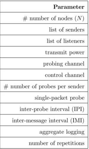
Table 3.1: Tridentper-round configuration parameters. Parameter

# number of nodes (N)

list of senders

list of listeners

transmit power

probing channel

control channel

# number of probes per sender

single-packet probe

inter-probe interval (IPI)

inter-message interval (IMI)

aggregate logging

number of repetitions

based on the needs of the experiment and the available storage. Finally, rounds and/or entire experiments can be repeated a configurable number of times, to increase statistical relevance.

As for metrics, not shown in the table,PDR,RSSI, and (if available)LQI are collected by default. If the platform allows, sender and receiver can acquire per-packet environmen-tal conditions such as noise floor, temperature, and humidity. These values are recorded according to the per-round logging policy.

Interacting with the nodes under experiment. Changing the per-round configura-tion parameters is not the only opconfigura-tion to interact in-field with nodes. Table 3.2 describes the commands available to the operator. As already mentioned, the operator can upload the description of an entire campaign configuration on the master, which then uses it to orchestrate the various rounds with the appropriate per-round configuration. However, the operator can also start and stop the execution of the experiment; these commands are propagated network-wide, with a mechanism similar to the one used to mark the start of a single round. Alternatively, the master node can be used to start and stop the experiments, e.g., using the on-board user button.

(45)

3.2. TRIDENT 25

Table 3.2: In-field commands.

Command Target Description

upload master load a campaign configuration

start network start the execution of an experiment

stop network stop the execution of an experiment

poll 1-hop query battery level

sleep 1-hop place nodes in low-power listening

wake-up 1-hop remove nodes from low-power listening

download(n) node download logs from selected node

erase(n) node erase flash of selected node

sniff operator toggle packet sniffing

or to start a new experimental campaign. Alternately, the operator can also put to (or wake-up from) sleep a subset of the nodes, and query for their battery level.

Other commands enable the operator to download the experiment logs from a selected node, and to erase its flash memory after successful data transfer is verified. Finally, passive packet sniffing can be activated on the node managed by the operator, enabling the latter to ascertain whether all nodes properly started the experiment.

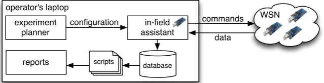
3.2.2 Toolset Overview

Figure 3.2 depicts the main structure of Trident. WSN nodes, the subject of the exper-iment, are programmed with a platform-specific mote-level runtime that is experiment-agnostic; its behavior is established by the operator without requiring any coding.

This configuration is performed through the GUI of a dedicated component, the exper-iment planner, which resides on the operator’s laptop. The experiment planner essentially enables the operator to quickly and easily define the various details of the experiment, by properly setting the values for the parameters in Table 3.1. This step does not need to be performed in-field, as the planner enables only the definition and storage of experiments. The actual upload of experiments to the master, and from there to the rest of the

in-field assistant

WSN

database

experiment planner operator's laptop

configuration commands

reports scripts

data

(46)

WSN, is instead supported by the in-field assistant, which also enables the execution of the other commands in Table 3.2. Communication with the WSN is enabled by a mote acting as a gateway, connected to the USB port of the operator’s laptop.

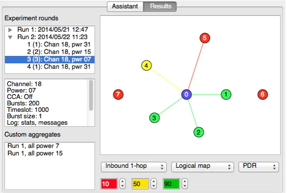
The in-field assistant provides also a simple visualization of the connectivity map built from available collected traces. An example is shown in Figure 3.3, visualizing the quality of the inbound links for node 0 according to a intuitive green/yellow/red color-coding, whose semantics in terms of PDR is configurable.

This feature is particularly useful whenTridentis used for a short-term assessment, as it quickly informs the operator about areas with connectivity problems, whose nodes can then be re-arranged. A similar visualization is provided also for mobile nodes; once the in-field assistant is fed with a sequence of locations, it can ”replay” the maps, showing to the operator how connectivity evolved due to mobility.

Finally, the database and associated plotting scripts simplify the storage of the col-lected data and its offline analysis. The database contains generic and customizable stored procedures for data manipulation. The set of pre-canned scripts allows the user to quickly plot trends derived from data collected, e.g., currently including network-wide

PDR, spatial and temporal variations of the metrics, correlation of PDR with RSSI and

LQI.

3.2.3 Platform-specific Details

Trident currently supports two hardware platforms: TMote Sky and Waspmote. The former directly integrates the CC2420 radio chip, while the latter relies on an exten-sion module for radio communications, in our case the XBee S2 integrating the

ZigBee-Figure 3.3: The “results view” of the Trident in-field assistant, showing one-hop inbound

(47)

3.2. TRIDENT 27

compliant EM250 system-on-chip. Both transceivers implement the 2.4 GHz IEEE 802.15.4 physical layer.

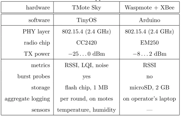
The software architecture of Tridentconfines the differences mostly in the platform-specific runtime installed on motes, although a few changes are needed also to parts of the in-field assistant handling communication with the WSN and parsing the logs for visualization. We refer to these platform-specific portions of the software as thebackend, and summarize the differences in Table 3.3. The Waspmote variant provides less features than the TMote Sky counterpart, as TinyOS allows low-level access to the radio chip while Waspmote provides only the high-level interface of the ZigBee application support sublayer (APS). These trade-offs are discussed in the rest of the section, along with other implementation details.

Available metrics. The two platforms provide different metrics. TinyOS recordsRSSI

and LQI for each received message, while the XBee radio module reports only RSSI. Moreover, unlike ZigBee, the low-level API available to TinyOS applications allows re-questingRSSI when the channel is idle to measure the noise floor.

The temperature and humidity sensor of TMote Sky provides important information for our studies of the environmental effects on connectivity. In principle, the same holds for Waspmote, given the wide range of sensors available for this platform. However, we have not yet implemented support for them in_Trident, although this does not pose any particular technical problem.

Experiment execution. On both platforms the experiment configuration is installed in the non-volatile storage of the master node. The TMote Sky backend supports uploading the configuration wirelessly or via USB, and stores it in a dedicated flash partition, while the Waspmote backend relies on a configuration file on the SD card.

Table 3.3: Platform support in Trident.

hardware TMote Sky Waspmote + XBee

software TinyOS Arduino

PHY layer 802.15.4 (2.4 GHz) 802.15.4 (2.4 GHz)

radio chip CC2420 EM250

TX power −25. . .0 dBm −8. . .2 dBm

metrics RSSI, LQI, noise RSSI

burst probes yes no

storage flash chip, 1 MB microSD, 2 GB

aggregate logging per round, on motes on operator’s laptop

(48)

As described in Section 3.2.1, the network is time-synchronized at the beginning of each round to avoid collisions among probes. The backends implement different techniques. In the case of TMote Sky, dissemination relies on a TDMA scheme where each node has its own time slots to repropagate commands, in a way similar to the mechanism outlined for probe transmission in Section 3.2.1. The common time reference needed for both the TDMA dissemination phase and to calculate tstart is established with TinyOS packet-level

time synchronization service [50], yielding sub-millisecond precision.

As ZigBee does not provide such a synchronization service, we rely on the standard multi-hop broadcast feature, basically a network flooding. However, based on the Zig-Bee Pro feature set [89], broadcast packets are always sent 3 times in a row, increasing reliability at the expense of energy consumption. These broadcast packets are separated by a 500 ms interval plus a random delay between 0 and 40 ms. Therefore, in the worst case where the start synchronization message is received only upon third attempt, the time synchronization error goes slightly above 1 s per hop.

To secure a collision-free transmission schedule the IPI should be set long enough to compensate for these synchronization errors and also for the time drift of the nodes. On TMote Sky the synchronization error is negligible; the typical time drift of 100 ppm results in two nodes drifting apart by 36 ms in half an hour. Therefore the use of 250 ms time slots during 30-minute rounds can be considered safe, counting also the time needed for internal processing of the received packets. Instead, on Waspmote the second-per-hop error should be compensated; we achieve this by using 3 s time slots.

Moreover, transmission of probes as one-hop broadcast requires an additional second, again due to the triple transmission performed by the ZigBee network layer. Therefore, it is impossible to send bursts of packets with Waspmote; on TMote Sky, bursts are instead supported with a configurable IMI, set to 20 ms by default.

(49)

3.2. TRIDENT 29

TX TX TX TX TX TX

? x ?

se nd er PHY re ce ive r PHY APP 0.5s

TX TX TX

x x ?

IPI

application-level packet arrival timestamps

1 2

APP 3

R1 R2 R3

RX 2 RX 1 RX 3

Figure 3.4: ZigBee transmits each broadcast packet three times.

two hypothetical experiment runs, one where each probe sent is always received upon first attempt, and one where it is received always upon the third attempt. The link-level

PDR would be a meager 33% in the second case, yet the application-levelPDR (the only directly measurable) would be 100% in both cases, providing a false representation of the quality of the wireless link.

Nevertheless, we can infer the number of failed attempts by looking at the packet ar-rival time, based on the fact that the three broadcast transmissions in ZigBee are spaced relatively far apart (500 ms). It is therefore possible to determine, upon receiving a broad-cast packet, whether this was the first, second, or third transmission. We confirmed this experimentally: Figure 3.5 shows the distribution of the packet arrival interval (modulo the nominal IPI) measured at the application level for an intermediate-quality link. For a perfect link, all packets would be received with the same IPI, 15 s in this case; however, this is not the case when packets are lost. Consider an application-level packeti, received on first attempt. If the previous packet, i−1, was received only on second or third at-tempt, the IPI between the two packets is smaller than 15 s. A similar reasoning holds in case the next packeti+ 1 is not received upon first attempt, yielding an IPI greater than 15 s. Clearly, the histograms to the left and right of the central one in Figure 3.5 can be generated also by intermediate combinations, e.g., if i is received upon second attempt and i+ 1 upon third, the IPI will be around 14.5 s.

Packet loss can be inferred by comparing the application-level packet arrival

times-0 500 1000 1500 2000

14000 14500 15000 15500 16000

packet arrival interval, ms

n

umber of pack

ets

(50)

tamps (e.g.,R1 andR2 in Figure 3.4), provided there is at least one packet in the received

sequence known to have arrived upon first attempt. This can be stated certainly when at least one pair of packets (not necessarily consecutive) has either the minimum or maximum possible recorded arrival interval (modulo the IPI), i.e., placed leftmost or rightmost on the histogram of Figure 3.5. Indeed, this means that the one of the packets was delivered on first attempt and the other on last, as in the case of R1 and R2.

In principle, it may happen that no such IPI is recorded during the whole test. In practice, this is unlikely to happen for intermediate-quality links. However, one can still infer the characteristics of the link based on the application-levelPDR. If the latter is very good, one can assume that the majority of the packets were received on the first attempt and base the analysis on this fact. For very bad links, it may be impossible to measure the actual PDR precisely when there are just few packets received from the whole sequence. Storing the experiment data. Due to the storage limitations of TMote Sky, per-probe logging can be replaced by storing per-round averages of the recorded values, computed on the nodes themselves. Waspmote does not have strict storage capacity limitation; full logs are always stored and the log analysis performed on the operator’s laptop. However, we plan to implement on-board log processing also on Waspmote, to reduce the downloading time of large logs.

3.3

Harpoon

Harpoon is the expressly designed tool to simplify the chore of in-field routing perfor-mance assessment. Currently, Harpoon supports two routing protocols: CTP (Collec-tion Tree Protocol) [33], arguably the de-facto protocol for data collec(Collec-tion applica(Collec-tions, and ORW (Opportunistic Routing Protocol) [41], a more recent opportunistic approach and competitor. _Harpoon collects common metrics and parameters for both protocols, as specified in Section 3.1.1 and a set of protocol-specific ones. For CTP, we acquire the

parent in the tree at every node at the time of sending a message, along with the total number of parent changes observed throughout the experiment. For ORW, we acquire the first neighbor, the number of dummy messages and the number of neighbors for each node.

Similarly to Trident, the tool supports interactive vs batch experiments and sup-porting a new routing protocol in the tool is simplified by its software architecture. The set of options to interact in-field with the nodes is much reduced in comparison with Trident, changing the per-round configuration parameters and downloading the data traces are the only options available to the operator.

(51)

3.3. HARPOON 31

of routing experiments, then provide an overview of theHarpoon toolset.

3.3.1 Experiments Execution

As in Trident, an entire experimental campaign with Harpoon is defined as a set of

rounds, each with its own configuration parameters. Each round has its own configuration parameters, detailed next. The time between two consecutive messages from the same

source node is the inter-probe interval (IPI).

Probing the network. Routing performance is assessed by having a set of nodes acting assources sending messages towards asink node. We instrumented the routing protocols implementation to provide our test application with the necessary hooks to gather the statistics and parameters mentioned in Section 3.1.1. We embed this information withing the application messages and report them to the sink. Unlike the connectivity assessment, transmissions are not centrally scheduled, the generation of messages being randomly scattered over time, as in most data collection applications [49]. During the experiment, Harpoon duty cycles the radio of the source nodes. We adopt the CTP default setting of having the sink node always on.

Sink node. The parameters describing the round configuration are disseminated by the

sink node at the beginning of each round. This node is the equivalent of the master

node from Trident. The sink receives an entire experimental campaign configuration via USB connection from operator’s laptop and dissemination to the WSN nodes is done using broadcast communication. This way, physical access to the nodes is not required in order to change or initiate an experimental campaign. Not only that it acts like a coordinator of the network, but the sink node also acts as an ”aggreg