Ground state and dynamical properties of many-body systems by non conventional Quantum Monte Carlo algorithms

(1)

UNIVERSIT `

A DEGLI STUDI DI TRENTO

Facolt`a di Scienze Matematiche, Fisiche e Naturali

Dipartimento di Fisica

Tesi di Dottorato di Ricerca in Fisica Ph.D. Thesis in Physics

Ground state and dynamical properties of

many–body systems by non conventional

Quantum Monte Carlo algorithms

Supervisor: Candidate:

Prof. Francesco Pederiva Alessandro Roggero

(2)

(3)

Introduction and

Motivations

The fundamental laws necessary for the mathematical treatment of large part of physics and the whole of chemistry are completely known, and the difficulties lies only in the fact that application of these laws leads to equations that are too complex to be solved.

Paul Dirac – 1929 A complete description of a quantum system composed by even a small number of interacting particles remains one of the most challenging problems in theoretical physics today. The main difficulty being the presence of interaction– induced correlations between particles, this in general forces the description of the state of the system to live in a space which is exponentially large in the number of degrees of freedom. Theoreticians realized the problem already in the early days of Quantum Mechanics as summarized in Dirac’s famous quote above.

A great effort as been dedicated in the past to the development of reliable approximations to thisQuantum Many–Body Problem(QMBP) with the hope of predicting properties of real systems starting only from the underlying physical theory, an approach that has come to be know asab–initio. For non–relativistic particles, which are the focus of the present work, this translates to solving the N–particle Schroedinger equation with the bare inter–particle potential. In some cases this approach can be attacked head–on since the inter–particle interaction is well–defined and known, such as the Coulomb potential between point–particles in Chemistry. In other cases, as the nuclear many–body problem, even the interaction between the effective degrees of freedom (the nucleons) is not known and thus a strictlyab–initiodescription is not possible. Nevertheless, once a choice has been made for the inter–particle interaction, the problem of solving the corresponding Schroedinger equation is perfectly well–posed and usually the term ab–initio is used for techniques that approximately solve it without introducing phenomenological parameters in the theory. This will be the methods we will focus on during this work.

The simplest N–body problem is the 1–body problem and then the first attempts to address the QMBP are mean–field theories that replaces the cor-related degrees of freedom of the particles with a collection of effective ones that (hopefully) don’t interact with each other, the so called quasi–particles. This clearly provides a huge simplification to the initial problem. Contrary to

(6)

what one may think at the beginning this approximation doesn’t work well only in weakly–correlated systems, but it may happen that, after changing basis to quasi–particles, theresidual interactionbetween them turns out to be very weak. Phonons in harmonic lattices are a simple example of this appealing behavior. A famous example of this kind of approach is the Hartree–Fock method [1, 2], a variational approach where the independent–particle assumption is encoded in the analytical form of the wave–function to be minimized: a Slater–determinant of single–particle states for fermions. In this way the HF solution represents the best approximation to the wanted solution of theN–particle Schroedinger equa-tion that can be written as a direct sum ofN 1–particle solutions.

The variational approach is very powerful and can be fruitfully employed also with variational wave–functions that explicitly contain correlations, providing a better description of the ground–state of the system. The technically challeng-ing task here is the evaluation of the cost–function that has to be minimized: the expectation value of the Hamiltonian on the correlated wave–function. Different methods have been developed in the years to deal with this problem, both de-terministically such as the Fermi–Hyper–Netted–Chain [3, 4] and stochastically such as the Variational Monte Carlo [5]. We will discuss more the Variational Monte Carlo technique in later chapters.

When the starting mean–field state is a good approximation of the true solu-tion one may also resort to some sort of perturbasolu-tion theory to add the missing correlations to the starting state. Many techniques have been developed in the past, from Many–Body Perturbation Theory [6] to methods that employ dia-gram resummations like Bethe–Bruekner–Goldstone theory [7], Self–Consistent Green’s Functions theory [8] and Coupled–Cluster (CC) theory [9] among the others.

It is also possible to include the effects of correlations without resorting to any series expansion by using stochastic methods like Quantum Monte Carlo [10]. The price to pay is the presence of statistical noise in all the predicted properties, noise that, thanks to the Central Limit Theorem (cf. Section 1.1), can be made arbitrarily small with more computation. These techniques are capable of providing exact results for strongly correlated bosonic systems and can be adapted to deal with fermionic degrees of freedom usually with just controllable approximations, and all this with a favorable (polynomial) scaling with system size. Quantum Monte Carlo (QMC) methods have now become standard tools for computations in a wide variety of strongly correlated systems [11] ranging from quantum chemistry [12, 13] to condensed matter [14, 15], and nuclear physics [16]. As example, some of the most accurate calculations for light nuclei and neutron matter were performed using continuum diffusion based QMC methods, i.e., nuclear Green’s function Monte Carlo (GFMC) and Auxiliary Field Diffusion Monte Carlo (AFDMC) [17, 18, 19, 20], in conjunction with the semi–phenomenological Argonne-Urbana family of nuclear forces [21, 22].

(7)

vii

Many–body methods that work on spaces generated by some set of single– particle states like the above mentioned Many–Body Perturbation Theory and Coupled–Cluster. As example of the advantages this brings, one of the draw-backs of CC theory is the non–variational nature of the calculated energy and more generally the difficulty of calculating expectation values using the wave– function obtained from the calculation; the availability of a QMC algorithm that work in the same space allows then not only variational estimates of the CC en-ergies but, even more interestingly, the possibility to calculate consistently any observable. Working in a discrete space brings also other enjoyable properties like the possibility to use non–local interactions in the calculations, something that with conventional methods is doable only at the price of introducing un-controllable approximations. The extension to these non–local interaction is essential for instance in Nuclear Structure where modern potentials derived in the framework of Chiral Effective Field Theory [25, 26, 27] are naturally of non–local character, at least at high enough order in the momentum expansion1. Extension of QMC to deal efficiently with these interaction is thus of pivotal importance in order to disentangle, by comparing with other techniques, the role played by the interaction from the effects coming from the many–body treat-ment employed. Besides the importance of pinpointing the nucleon–nucleon interaction, an everlasting challenge in nuclear theory, accurate results can be obtained to constrain effective theories (like e.g. Density Functional or Rela-tivistic Mean Field Theory) that may be then employed to study systems whose complexity is far beyond the reach ofab–initiocalculations (cf Section 3.2). As example the homogeneous part of Density Functionals used in Chemistry for electronic structure calculations [29] is fitted to reproduce accurate Quantum Monte Carlo results for the electron gas [30].

The second main topic addressed in this work is the computation of dy-namical properties of strongly interacting Many–Body systems. Many impor-tant physical properties of matter, from viscosity to magnetic susceptibility, are closely linked to the underlying microscopic dynamics. Understanding the details of this microscopic dynamics is thus one of the fundamental goals of Many–Body theory. A big drawback of QMC methods is however their inability to treat in a reliable way dynamical properties of quantum systems, this failure is essentially linked to the fact that QMC works in imaginary-time (see Section 1.2.1) so for quantities that do not directly translate into imaginary-time lan-guage the noise can be hardly reduced and calculations becomes unfeasible. The usual way to turn around that problem is to compute quantities in imaginary-time first and then use analytic–continuation into the real imaginary-time, this procedure is accomplished by an inverse Laplace transform of noisy data, a notorious ill-posed problem [31, 32, 33].

Even if useful in sometimes as we shall see, this approach breaks–down in many interesting cases; for example the probably most notorious failure is that even the more sophisticated inversion scheme, the Maximum Entropy Method, cannot resolve the double peaked structure of the dynamic structure factor of superfluid He4 (see Fig 1). Only very recently [34] this two–peak structure has been obtained trough the inversion of imaginary–time data with a novel inver-sion technique know as Genetic Inverinver-sion via Falsification of Theories (GIFT).

1_{see however [28] for a recent attempt to incorporate chiral interactions in continuum QMC}

(8)

Figure 1: Dynamical structure factor for liquid He4 at 1.2 K and wavelength

Q=0.76A−1. Solid line as measured by neutron scattering [36]; dashed curve MEM reconstruction from the PIMC data [37]

Also recently, an hybrid semiclassical–PIMC calculation as been carried out to study the high-momentum response function in this system with encouraging results [35], it is however difficult to extend such results to the low–momentum transfer region that we are interested in. In this work we try to devise a method to alleviate these problems by adopting the Integral Transform approach on which is based the LIT method [38], now a powerful tool to study dynamical properties of few body nuclear systems and one of the few capable to address problems in the continuum part of the hamiltonian spectrum. The idea is to replace the commonly used Laplace transform with a different one that is more suitable to obtain stable inversions.

The thesis is structured with a first chapter that introduces the relevant no-tions at the foundation of Monte Carlo methods and present the key algorithms in a general basis–independent fashion. We will then specialize in Chapter 2 to our Diffusion Monte Carlo in Fock–space and then present applications to nuclear–system with non–local Chiral interactions in the following chapter. We will then present in Chapter 5 the techniques used for the calculations for the superfluid He4_{system, with a focus on bosonic systems only. Chapter 4 reviews}

(9)

Chapter 1

Monte Carlo Methods

Solving the Schroedinger for an interacting many–body system is a really chal-lenging task, the aim of this chapter is to introduce the stochastic techniques used in this work to pursue this goal. To set the stage let us start by consid-ering a somewhat simpler, but technically still very challenging, problem: the calculation of expectation values on a correlatedN–body wave–function Ψ(R)

⟨O⟩φ= ∫

dRΨ∗(R)O(R)Ψ(R)

∫ dR∣Ψ(R)∣2 (1.1)

whereR is 3N–dimensional vector and for simplicity we have consideredO to be a local operator. The evaluation of the above expression is a formidable task already for small numbers of particles mainly due to the dimensionality of the problem. Stochastic techniques can however be employed if we interpret the above expectation value as an average over a suitable Probability Density Func-tion (PDF) defined over this 3N–dimensional space. The great advantage in this strategy is that, thanks to the Central Limit Theorem, the error on the stochas-tic estimator obtained fromM sampled configurations scales aserr(M) ∝M−12

regardless of the dimensionality of the problem.

This favorable scaling of computational time with system size, while pre-serving at the same time the capability of accurate results, has motivated the adoption of Monte Carlo techniques in many fields of Physics. Classical systems in thermal equilibrium can be efficiently tackled by Classical Monte Carlo tech-niques, which are exact methods to sample from the Boltzmann distribution at finite temperature. For quantum systems, in the last two decades Quantum Monte Carlo (QMC) methods have become a standard tool for computations in a wide variety of strongly correlated systems [11] ranging from quantum chem-istry [12, 13] to condensed matter [14, 15], and nuclear physics [16]. QMC are generally methods to solve the Schroedinger equation of non-relativistic Quan-tum Mechanics, and these will be the methods that we will focus most in this presentation. The applicability of stochastic integration to solve partial differ-ential equation comes from the fact that we can map a differdiffer-ential equation into a corresponding integral one (using e.g. Green’s functions) and this is the problem that we are actually going to solve. Monte Carlo methods can also be applied in relativistic theories and are in practice the only viable method to treat the low-energy non perturbative limit on Quantum Chromo Dynamics[39].

(10)

In the next section we will present the basic ideas of Monte Carlo sampling by presenting the Variational Monte Carlo method. We then focus on Projection Monte Carlo techniques that will be used to solve the Schroedinger equation.

1.1

Introduction

The first, natural, application of stochastic integration ideas to Quantum Me-chanics is for the computation of expectation values of the form:

⟨O⟩φ=

⟨φ∣Oˆ∣φ⟩

⟨φ∣φ⟩

=∫ dν⟨φ∣ν⟩⟨ν∣Oˆ∣φ⟩ ∫ dν⟨φ∣ν⟩⟨ν∣φ⟩

≡∫ dνφ∗(ν) (Oφˆ ) (ν) ∫ dν∣φ(ν)∣2 ,

(1.2)

where for convenience we have introduced a complete set of states_∫ dν∣ν⟩⟨ν∣. As mentioned in the introduction to this chapter, we have to express this ex-pectation value in a form suitable for MC integration:

⟨O⟩φ=∫

dνφ∗(ν) (Oφˆ ) (ν)

∫ dν∣φ(ν)∣2

=∫ dνφ

∗₍_ν₎φ(ν)

φ(ν)(Oφˆ ) (ν)

∫ dν∣φ(ν)∣2

= ∫ dν ∣φ(ν)∣

2

∫ dν∣φ(ν)∣2

ˆ

Oφ φ (ν)

= ∫ dν f(ν)o(ν) ≡_Ef[o(X)]

(1.3)

which can be interpreted as the expected value of the functiono(ν) =Oφˆ (ν)/φ(ν)

over the perfectly valid (ie. positive–definite and normalized) Probability Den-sity Function f(ν). The basic tool that we need is then to have the ability to generate samples from some known PDF f. Fortunately there are general purpose techniques for generating random numbers with the proper distribution such as the Markov Chain Monte Carlo. The idea is to generate a sequence of random configurations, with the next one depending only on its predecessor, in such a way that asymptotically these configurations are distributed according tof. If we start from a configurationXithe probability to end up in the

config-urationYi after the step can be described by a stochastic matrixM(Xi, Yi)and

one can show that the asymptotic distribution sampled by such process is the dominant right–eigenvector of the matrixM. Metropolis et al. [40] proposed a constructive way for generating M given the target densityf, it relies on the factorization of the matrix

M(Xi, Yi) =T(Xi, Yi)A(Xi, Yi) (1.4)

(11)

1.1. INTRODUCTION 3

The key finding is that, regardless of both Tand the target distribution f, if we choose forAthe following form

A(Xi, Yi) =min[1,

T(Xi, Yi)f(Yi) T(Yi, Xi)f(Xi)

], (1.5)

then the random process will produce samples distributed according tof. The configurations undergoing this random process will be calledwalkers. The role of the transition matrix is to control the efficiency of the overall process since low acceptance probabilities will reduce the number of samples effectively generated [41] (see also [42]).

Moreover, the fact that PDFs enter as a ratio in (1.5) allow us the great simplification of neglecting completely the normalization factor: f(ν) ≡ ∣φ(ν)∣2. The Monte Carlo estimator of expression (1.3) is then obtained as an arith-metic sum

̃ ⟨O⟩_φ= 1

M

∑

i=1

OL(νi) (1.6)

of so–calledlocalobservables:

OL(νi) = ⟨

νi∣Oˆ∣φ⟩

⟨νi∣φ⟩

= ∫ dµ⟨νi∣Oˆ∣µ⟩⟨µ∣φ⟩

⟨νi∣φ⟩

(1.7)

evaluated on theM configurations νi sampled fromf(ν).

This approach is clearly useful when we have access to some complicated wave functionφand we have no other practical way of computing the expecta-tion value (1.2). It is also extremely useful for finding good approximaexpecta-tions for the ground–state of interacting many–body Hamiltonians, and is in this con-text that is usually referred to as Variational Monte Carlo (VMC) [5]. In the particular case ˆO=Hˆ we have in fact avariational theorem

E0=⟨

Φ0∣Hˆ∣Φ0⟩

⟨Φ0∣Φ0⟩

≤⟨φ∣Hˆ∣φ⟩

⟨φ∣φ⟩ =Eφ (1.8)

where Φ0 is the ground–state wave–function and the equality holds only in the

caseφ≡Φ0. The above relation can then be used to choose the best

approxima-tion to Φ0 among a parametrized family of wave–functionsφ(α1, α2, . . .). The

power of the method relies in the great flexibility on the choice of the wave– functions that can explicitly incorporate correlations. This extremely accurate wave–functions usually depend on a large number of parameters [43] and need to be optimized trough suitable minimization schemes [44, 45, 46].

(12)

1.2

Projection Monte Carlo Algorithms

We will now turn to the Quantum Monte Carlo methods that will be used to find the ground–state of interacting many–body hamiltonians: Diffusion Monte Carlo and Reptation Monte Carlo.

In the introduction we have seen how to produce a random process that samples a known target density f by properly crafting a stochastic matrix M

of which f is the dominant right–eigenvector. The same ideas can be however applied also for the opposite process: producing a random process that will produce the dominant right–eigenvector of a known matrix. This is exactly the same idea underlying the so–called Power Method (PM) for finding the eigenvector corresponding to the biggest eigenvalue of a given matrixM:

1. start with some initial vector v0

2. apply the matrix (matrix–vector multiplication) ˜vk+1=Mvk

3. normalize the resulting vector vk+1=˜vk+1/∥˜vk+1∥

4. check for convergence (vk+1≈vk), if not go back to 2.

The main difference is that step 2. will be done stochastically stochasti-cally using Monte Carlo and thus we can treat extremely big (in many cases also infinite–dimensional) matrices, provided the matrix we are dealing with is sufficiently sparse. The PM is expected to work whenever we have a finite gap between the dominant eigenvalue and the rest of the spectrum and also when that eigenvalue is not degenerate. The rate of convergence of this scheme is however usually rather slow (≈ linear), but we can improve on it by noticing that the algorithm works even if instead of just multiplying the matrix M in step 2. we apply any monotonic function of it. A more efficient choice, provided its action on the current vector is easily computable, would be to use an expo-nential ofM. In this way we can hope for an exponential convergence towards the wanted solution.

1.2.1

Diffusion Monte Carlo (DMC)

Diffusion Monte Carlo is probably the most widespread variant of QMC for zero–temperature ground-state calculations of strongly correlated systems. The goal is to solve the time–independent Schroedinger equation producing samples distributed according to the ground-state wave-function, once these are available we can calculate relevant expectation values over it. The starting point is the (imaginary)time–dependent Schroedinger equation (t→iτ):

− ∂

∂τ∣Ψ(τ)⟩ =

ˆ

H∣Ψ(τ)⟩ = (Kˆ+Vˆ)∣Ψ(τ)⟩ (1.9)

where in the last expression we have explicitly separated the contributions ˆK

(13)

1.2. PROJECTION MONTE CARLO ALGORITHMS 5

(1.9) into the following integral equation:

⟨µ∣Ψ(τ+∆τ)⟩ = ∫ dν⟨µ∣Gˆ∆τ∣ν⟩⟨ν∣Ψ(τ)⟩

= ⟨µ∣e−∆τHˆ∣Ψ(τ)⟩

(1.10)

where we employed complete sets of states ∣ν⟩ and ∣µ⟩ for convenience. In the last equation ˆG∆τ is the Green’s function of equation (1.9), the so–called imaginary-time propagator. All eigenvectors of the Schroedinger equation would be solutions of Eq. (1.10), but we can isolate the eigenvector with the lowest eigenvalue∣Φ0⟩by looking at the long imaginary–time solution, in fact:

lim

τ→∞∣Ψ(τ)⟩ =τlim→∞e

−τHˆ_∣_Ψ₍₀_)⟩

= lim

τ→∞∑_n e

−τ En∣_Φ

n⟩⟨Φn∣Ψ(0)⟩

→e−τ E0∣_Φ

0⟩⟨Φ0∣Ψ(0)⟩ ∝∣Φ0⟩

(1.11)

where we have used the complete set of eigenstates of the hamiltonian∣Φn⟩, with

corresponding eigenvalues En. The expression in the last line holds provided

that the initial condition ∣Ψ(0)⟩ is not orthogonal to ∣Φ0⟩. In general, the

infinite imaginary–time limit will project out the lowest eigenstate that is not orthogonal to ∣Ψ(0)⟩, this can be used for instance to perform calculations of low-lying excited states with definite symmetry properties.

By repeatedly integrating (1.10), starting from some initial ansatz for the wave-function, we will project to the eigenstate of ˆH with the lowest eigenvalue as in the PM algorithm outlined above. An important, tough rather techni-cal point, is the renormalization at step 3. of the Power Method: without it the procedure would be extremely unstable leading eg. to zero–norm results. Preserving the norm of the solution along the projection is thus an essential ingredient for the stability of the method.

In the language used for DMC this renormalization step is applied by means of an iteration–dependent multiplicative factor Λkattached to the bare

propaga-tor that needs to be adjusted to preserve the normalization of the wave–function. In the usual case when the propagator is of exponential form, like in (1.10), this can be casted into an iteration–dependent energy shiftE_{T k}:

e−τHˆ Ð→Λke−τ ˆ

H_≡_e−τ(Hˆ−ET k)_. _(1.12)

For simplicity of notation, in the following we will use justET instead ofET k.

From Eq. (1.11) it is also easy to realize that with this choice ET → E0 for

sufficiently long projection times and we can thus use its average value as an estimate of the ground–state energy, thegrowth–estimator.

The main difficulty in the case of DMC with respect to the Power Method for finite, small matrices is to find an efficient way to compute the action of the imaginary–time propagator on a given state∣Ψ⟩. To appreciate better the issue, let us first rewrite the imaginary–time Schroedinger equation (1.9) in a slightly different fashion:

− ∂

∂τΨ(τ, ν) = ∫ dµ⟨ν∣

ˆ

H∣µ⟩Ψ(τ, µ)

= ∫ dµ⟨ν∣HˆT∣µ⟩Ψ(τ, µ) + ⟨ν∣HˆR∣ν⟩Ψ(τ, ν)

(14)

where in the second line we have explicitly separated the hamiltonian ˆH into a part that give rise to transitions ˆHT and another one that acts as a multiplicative

operator rescaling the PDF ˆHR. Obviously this splitting is basis-dependent, i.e.

operators that act as ˆHT in coordinate–space may act as an ˆHRin momentum–

space (eg. the kinetic energy).

Correspondingly the master equation (1.10) governing the evolution of the probability distribution Ψ(τ, ν)can be conveniently written as:

Ψ(τ+∆τ, ν) = ∫ dµ⟨ν∣G∆τ∣µ⟩Ψ(τ, µ)

= ⟨ν∣GR_∆τ∣ν⟩ ∫ dµ⟨ν∣GT_∆τ∣µ⟩Ψ(τ, µ)

=GR∆τ(ν) ∫ dµ G T

∆τ(µ, ν)Ψ(τ, µ).

(1.14)

Given a choice of basis, and consequent splitting in ˆHT and ˆHR, we can

inte-grate the evolution equation using for instance the Metropolis acceptance/rejection scheme explained before. Starting with a given configuration ∣µ⟩we propose a new move according to some transition probabilityT(µ→ν), use the MRT test (cf. Eq. 1.5) onGT_∆τ(µ, ν)with acceptance probability

A(µ→ν) =min[1,T(ν→µ)G

T ∆τ(µ, ν)

T(µ→ν)GT ∆τ(ν, µ)

] (1.15)

and attach a weightGR

∆τ(ν)on the proposed new configuration. If the

fluctu-ations of these weights are not too strong it may be sufficient to preserve the weights along the entire random–walk by accumulating them from one step to the next. This approach is however usually impractical since expectation val-ues calculated along the walk will be dominated by the few walkers with the bigger weights, wasting most of the computing power. A better approach is instead to interpretGR_∆τ(ν)as a survival, orbranching, probability. There are different ways of implementing this idea, the most popular one is to choose to work with walkers with weightw≡1: after the propagation and the measure of observables, the j–th walker with weightwjis replicatednj=int(wj+ξ)times,

whereξis a uniformly distributed random number in(0,1). The total number of walkers present in the population will keep changing during the evolution and its average dimension is set by properly tuning the energy shiftET.

The Metropolis step is extremely useful since it can be applied to a variety of ˆHT at the price to have low acceptance rates for poor choices of the auxiliary

probability T. This can be avoided, obtaining an acceptance rate of 100%, if we are capable of sampling directly from the transition probabilityGT_∆τ(µ, ν). This will be for instance the case for the CIMC algorithm described later in this work.

(15)

1.2. PROJECTION MONTE CARLO ALGORITHMS 7

expression for the ground state energy will be:

E0= lim τ→∞

⟨ΨI∣Heˆ −τ ˆ H_∣_Ψ

I⟩

⟨ΨI∣e−τHˆ∣ΨI⟩

=⟨ΨI∣Hˆ∣Ψ(τ)⟩

⟨ΨI∣Ψ(τ)⟩

= EΦ0[ΨI(X)EL(X)]

EΦ0[ΨI(X)]

(1.16)

where ΨI ≡Ψ(τ=0)and we have defined the local–energyELin some

configu-ration∣µ⟩as:

EL(µ) = ⟨

µ∣H∣ΨI⟩

⟨µ∣ΨI⟩

. (1.17)

The corresponding sample estimator will then be:

̃

E0= ∑ M

i EL(Xi)ΨI(Xi)

∑M

i ΨI(Xi)

. (1.18)

The same procedure can be carried out for general operators

ODM C=

⟨ΨI∣O∣Φ0⟩

⟨ΨI∣Φ0⟩

Ð→ ̃ODM C= ∑ M

i OL(Xi)ΨI(Xi)

∑M

i ΨI(Xi)

.

(1.19)

We note that (1.19) will be exact only for observables that commute with the hamiltonian, otherwise it will not be the wanted expectation value but amixed– estimator of it. This estimator will have a bias that depends on how much different is the trial function ΨI with respect to the ground state Φ0, this bias

will be however smaller than the variational estimate (1.3). There are ways to partially circumvent this within DMC usingextrapolated estimatorsor tech-niques such asforward–walking[48, 49, 50, 51].

Efficiency issues and Fermions

The separation carried out before Eq. (1.13) is useful also because we need different conditions on ˆHR and ˆHT to have an efficient algorithm:

• the transition to new states governed by ˆHT should be implementable in

an efficient way

• the values of the rescaling factor given by ˆHR should not fluctuate too

much during the evolution (ie. it has to have a finite variance)

Clearly these conditions depend strongly on the chosen basis, but there are general–purpose techniques that can help for both, one of them being Impor-tance Sampling (IS) which is more extensively presented in Appendix A. Given the target hamiltonian ˆH and an auxiliary, for now indeterminate, state ∣ΦG⟩

we can consider the following similarity transformation:

⟨ν∣Hˆ∣µ⟩ Ð→ΦG(ν)⟨ν∣Hˆ∣µ⟩Φ−G1(µ) ≡ ⟨ν∣HIS∣µ⟩ (1.20)

(16)

The spectrum of both hamiltonians will be the same but, with a proper choice of the auxiliary state∣ΦG⟩, the similarity–transformed one can be much

more easy to deal with. Consider for now the long imaginary–time behavior attained by using the propagator of ˆHIS for the evolution:

lim

τ→∞ΨIS(τ, ν) =τlim→∞⟨ν∣e

−τHˆIS∣_Ψ(₀)⟩

= lim

τ→∞∑_n e

−τ En⟨_Φ

n∣Ψ(0)⟩Φn(ν)ΦG(ν)

→e−τ E0⟨_Φ

0∣Ψ(0)⟩Φ0(ν)ΦG(ν) ∝Φ0(ν)ΦG(ν)

(1.21)

we see then that the asymptotically sampled distribution will be the product

P_∞(ν) = Φ0(ν)ΦG(ν). We recognize that if we choose ΦG ≡ Φ0 this method

reduces to a VMC calculation on the true ground–state distribution Φ2₀ (cf. Eq. 1.3).

The single step evolution with importance sampling becomes then:

Ψ(τ+∆τ, ν) = ∫ dµ⟨ν∣G∆τ∣µ⟩

ΦG(ν)

ΦG(µ)

Ψ(τ, µ)

= ∫ dµ⟨ν∣GIS_∆τ∣µ⟩Ψ(τ, µ)

(1.22)

and we see that the transition to the new state inνis now weighted with a factor

wIS(ν, µ) =ΦG(ν)/ΦG(µ). It’s main effect is to define a privileged direction for

the transitions: propagation towards states that enhance the weight wIS will

be favored while the probability to go in states that diminish this weight will be lowered.

It is easy too see that in the limit ΦG→Φ0we will gain a lot in efficiency since

the random walk will be pushed towards regions where Φ0 is big. This helps

us in increasing the efficiency of the transitions governed by the off–diagonal part of the ˆHT hamiltonian. It usually also helps in lowering the variance of

the reweight factor generated by ˆHRsince, in general, this weight is≈constant

in region where Φ0 is big, but to elaborate on that we need to specialize the

discussion to a particular basis as we will do in the next chapters.

However, IS not only helps in lowering variances, it may allow us to perform simulations even in cases where naively we would think to have no chance. Consider for instance the situation where

⟨ν∣G∆τ∣µ⟩ <0 for some µ, ν (1.23)

and so it cannot be interpreted as a PDF itself. With a proper choice of ΦI we

may have

⟨ν∣GIS_∆τ∣µ⟩ >0 (1.24) in those points. Unfortunately cases like (1.23) are not very rare, on the contrary we will be in that situation in almost all calculations involving fermions (with few notable exceptions) due to the Pauli statistics that forces the wave–function to change sign under the action of the permutation groupSN. This is the source

of the infamous fermion sign–problem. However, it is unlikely that we will be able to find some state ΨG for which ⟨ν∣GIS∆τ∣µ⟩ >0 in the whole Hilbert space

(17)

1.2. PROJECTION MONTE CARLO ALGORITHMS 9

This procedure is known in literature as the fixed–node approximationand its impact can be controlled by the quality of the guiding state ΨG.

Before going to the next algorithm we report the expressions for the energy and for the observables in the case where Importance Sampling is employed. The ground–state energy will now be:

E0=

EΦ0ΦG[

ΨI(X)

ΨG(X)EL(X)]

EΦ0ΦG[

ΨI(X)

ΨG(X)]

(1.25)

and we will have the following sample estimator:

̃

E0=

∑M

i EL(Xi)_ΦΨI(Xi)

G(Xi)

∑M i

ΨI(Xi)

ΦG(Xi)

(1.26)

with the local–energy as defined before. Analogously for a general observable:

̃

ODM C =

∑M

i OL(Xi) ΨI(Xi)

ΦG(Xi)

∑M i

ΨI(Xi)

ΦG(Xi)

. (1.27)

In the particular case where the trial and guiding wave–functions are the dame ΨI ≡ΦG we find the simplified expressions

̃

E0=

1

M

∑

i

EL(Xi) (1.28)

and

̃

ODM C=

1

M

∑

i

OL(Xi). (1.29)

Further developments along these lines require some knowledge of the basis actually used in the calculation and will be explored when relevant.

1.2.2

Reptation Monte Carlo (RMC)

Reptation Monte Carlo (RMC) is another Projection Monte Carlo method based on a path–integral representation of the imaginary time projector. We start by choosing an imaginary–time interval (or inversetemperature)β, big enough that we can assume convergence to the ground–state so that:

Z(β) = ⟨ΨI∣Ψ0⟩

= ⟨ΨI∣e−β ˆ H_∣_Ψ

I⟩

(1.30)

for some appropriate initial trial–state ΨI. Inserting identities using a complete

basis 1= ∫dµ∣µ⟩⟨µ∣we can decompose (1.30) into Kslices:

Z(β) = ⟨ΨI∣∫ dµ0∣µ0⟩⟨µ0∣e−β ˆ H

∫ dµK∣µK⟩⟨µK∣ΨI⟩

= ∫ dµ0. . . dµK⟨ΨI∣µ0⟩⟨µ0∣e−

β

KHˆ∣_µ₁⟩⟨_µ₁∣_{. . .}∣_µ_K₋₁⟩⟨_µ_K₋₁∣_e− β

KHˆ∣_µ_K⟩⟨_µ_K∣_Ψ_I⟩

= ∫ dµ0. . . dµKΨI(µ0)⟨µ0∣G∆τ∣µ1⟩⟨µ1∣. . .∣µK−1⟩⟨µK−1∣G∆τ∣µK⟩ΨI(µK)

(18)

where G∆τ the same Green’s function defined in (1.10) and ∆τ ≡β/K. The

quantity Z(β) is then interpreted as partition function, and imaginary–time

pathsX = {µo, . . . , µK} are given the normalized probability:

Π[X ] = ΨI(µ0)⟨µ0∣G∆τ∣µ1⟩⟨µ1∣. . .∣µK−1⟩⟨µK−1∣G∆τ∣µK⟩ΨI(µK)

∫ dµ0. . . dµKΨI(µ0)⟨µ0∣G∆τ∣µ1⟩⟨µ1∣. . .∣µK−1⟩⟨µK−1∣G∆τ∣µK⟩ΨI(µK)

.

(1.32) We may also introduce a path–actionS[X ] and write simply:

Π[X ] = e

−S[X ]

Z(β). (1.33)

There are many ways for sampling such imaginary–time paths X using Markov Chain Monte Carlo techniques with MRT sampling. Given an initial pathX, a new oneY is proposed according to some probabilityT(X → Y)and the move is then accepted/rejected according to the Metropolis probability

A(X → Y) =min[1,T(Y → X )Π[Y]

T(X → Y)Π[X ]]. (1.34) The versatility of this method comes from the relatively large freedom in the choice of the proposal probability T(X → Y), also enlarged by the possibility of using the importance sampled propagator (1.22) with Φg ≡ ΨI to obtain

equivalent expressions shifting the ΨI along the path. In the original algorithm

[52] for instance, one proceeds by taking in initial path X and then chooses at random a growth direction. This defines a headslice and a tail slice of the path. A numberδof slices are then added to theheadand removed from thetail

generating a new pathY. The generation of the new slice is performed sampling

δsteps directly from the Green’s functionG∆τ(µ, ν)(or its IS equivalent). This

”reptile”–like movement of the path, which simplifies the calculation of the ratios in (1.34) together as giving a reasonable acceptance rate, has given the name to Reptation MC. We will explore some slight variations of this sampling method when we will implement it in coordinate–space later on.

The appealing properties of RMC are the fact that it allows to have access to the ground–state energy with an accuracy comparable to DMC while at the same time allowing for the exact evaluation of other observables. Lets consider for instance the expression for the total energy obtained on a random walk starting at∣Ψ(τ=0)⟩ =∣ΨI⟩after a total propagation timeβ:

E(β) = ⟨ΨI∣Heˆ −

τHˆ_∣_Ψ I⟩

⟨ΨI∣e−τHˆ∣ΨI⟩

= ⟨ΨI∣Hˆ∣Ψ(τ)⟩

⟨ΨI∣Ψ(τ)⟩

= ⟨ΨI∣e−

β

2HˆHeˆ −

β

2Hˆ∣Ψ_I⟩

⟨ΨI∣e−βHˆ∣ΨI⟩

= ⟨Ψ_⟨(β/2)∣Hˆ∣Ψ(β/2)⟩

Ψ(β/2)∣Ψ(β/2)⟩

(1.35)

(19)

1.2. PROJECTION MONTE CARLO ALGORITHMS 11

Figure 1.1: Potential energy along a K =800 slices-long imaginary-time path (from [53] )

we can calculatepureestimators for general operators by measuring in the cen-tral slice of the path:

O(β) = ⟨ΨI∣e

−β

2HˆOeˆ −

β

2Hˆ∣Ψ_I⟩

= ⟨Ψ(β/2)∣Oˆ∣Ψ(β/2)⟩ ⟨Ψ(β/2)∣Ψ(β/2)⟩

β→∞

ÐÐÐ→⟨Ψ0∣Oˆ∣Ψ0⟩

⟨Ψ0∣Ψ0⟩

(1.36)

and then use the following estimator:

˜

O= 1 M

M

∑

i

OL(XKi/2) (1.37)

where with the notation Xi

m we indicate the m–th slice of the i–th path Xi

sampled and in the last line we have assumed to using the importance– sampled Green’s function for the sampling with ΨG≡ΨI(so that the denominator is≡1).

The average value of the observableO, if we measure it away from the center, will converge to its mixed–estimator value at both the endpoints of the path. In Fig.1.1 we see for instance the expectation value of the potential operator along aK=800 slices for a bulk system of superfluid He4going from its mixed value at the edges to the exact value in the middle. Note that the curvature has not to be always positive due to the fact that the mixed–estimator does not satisfy any variational principleOmix≥O0(contrary to the energy).

(20)

functions:

CO(τ;β) =

⟨ΨI∣e−

β

2HˆOeˆ −τHˆOeˆ −

β

2Hˆ∣Ψ_I⟩

=⟨Ψ(β/2)∣Oeˆ −τ

ˆ

H_Oˆ_∣_Ψ₍_β_/₂_)⟩

⟨Ψ(β/2)∣Ψ(β/2)⟩

β→∞

ÐÐÐ→⟨Ψ0∣Oeˆ −τ ˆ H_Oˆ_∣_Ψ

0⟩

⟨Ψ0∣Ψ0⟩

=⟨Ψ0∣Oˆ(0)Oˆ(τ)∣Ψ0⟩

⟨Ψ0∣Ψ0⟩

(1.38)

where the time–dependence in the last expression is in the Heisenberg picture. In order to estimate this quantity we can consider longer paths composed by

P =K+Q time slices withQ=τ/∆τ and evaluate the operators in two slices separated by an intervalQ:

̃

CO(τ=Q∆τ) =

1

M

∑

i

OL(XKi /2)OL(XKi /2+Q). (1.39)

In the last expression we kept the observables in the innermost part of the ”snake” in order to minimize the effects coming from the necessary use of the importance function ΨI.

(21)

Chapter 2

DMC in

Slater–Determinant space

The great success of Quantum Monte Carlo for fermionic systems (employing the fixed–node prescription) is largely because of the development of high–quality trial wave functions. However, most of these wave functions have forms which are convenient only for calculations in coordinate–space. The lack of accurate and computationally efficient trial ground-state wave functions has, thus far, precluded a wide exploration of these algorithms within the configuration inter-action (CI) scheme (see, however, [54]). Generally, QMC methods within the CI scheme tend to rely on auxiliary fields introduced via the Hubbard–Stratonovich transformation [55, 56, 57, 58, 59]. Much recent interest, however, was sparked by the demonstration that even within the CI scheme it is possible to apply stochastic projection to systems much larger than what would be possible using conventional matrix diagonalization [60]. And moreover, working in CI–space allows the development of exciting hybrid algorithms like the Semistochastic Quantum Monte Carlo [61] that combines exact diagonalization in a restricted sub–space with stochastic projection trough Monte Carlo.

In this chapter we present the details of our implementation of Diffusion Monte Carlo in a CI–space, the Configuration Interaction Monte Carlo (CIMC), presenting also some first applications.

2.1

Random walk on a Fock–space

Let us take a finite setS of sp states of sizeNsand consider a general second–

quantized fermionic Hamiltonian which includes two and possibly many–body interactions

H = ∑

i∈S

ia†iai+ ∑ abij∈S

V_ijaba†_aa†_baiaj+. . . , (2.1)

where a†_i creates a particle in the single-particle (sp) state labeled by i (i is a collective label for all sp quantum numbers) and theV_ijab are general (anti– symmetrized) two-body interaction matrix elements:

Vijab= ⟨ij∣Vˆ∣ab⟩ − ⟨ij∣Vˆ∣ba⟩ ≡ ⟨ij∣∣ab⟩. (2.2)

(22)

The resulting many–body Hilbert space would be spanned by the full set of N–particle Slater determinants that can be generated using the sp orbitals

i∈ S. We will denote these Slater–determinants in the occupation number basis by∣n⟩, wheren≡ {ni}andni=0,1 are occupation number of the single–particle

statei. In this Hilbert space we can express the one–time step evolution as Ψτ+∆τ(m) = ∑

n

⟨m∣Pˆ∣n⟩Ψτ(n) (2.3)

where Ψτ(n) ≡ ⟨n∣Ψτ⟩is the representation of the wave–function in this basis.

Our goal is to perform the evolution in Eq.(2.3) in a stochastic way. In order to do this, let us first split the matrix elements of ˆP as follows

⟨m∣Pˆ∣n⟩ =p(m,n)g(n) (2.4) with

g(n) = ∑ m

⟨m∣Pˆ∣n⟩ (2.5)

and

p(m,n) = ⟨m∣

ˆ

P∣n⟩

∑m⟨m∣Pˆ∣n⟩

(2.6) .

Now if the matrix elements⟨m∣Pˆ∣n⟩ ≥0 we can interpretp(m,n)for fixedn

as (normalized) probabilities andg(n)as a weight factor. This is analogous to what happened in conventional coordinate–space formulations where the prop-agator is splitted into an off–diagonal part times a weight factor.

Imagine that at a given imaginary–time τ the wave–function Ψτ is non–

negative in configuration space (ie. Ψτ(n) ≥0), then we can represent it as an

ensemble of configurations. Due to the non–negativity of the matrix elements of

P, we also have that the evolution described in Eq.(2.3) preserves the signs, ie. Ψτ+∆τ(m) ≥0∀m. This suggests the following procedure for the imaginary–

time evolution: given the current configuration n a new configuration m is chosen from the probability distributionp(m,n)and its weight gets multiplied byg(n). In order to improve efficiency the latter is usually substituted with a

branchingstep where the new configuration inm is replicated according to the integer value of its weight.

In practice one has to choose some form for the evolution operator that appears in Eq.(2.3), a common choice in discrete spaces is the following

⟨m∣Pˆ∣n⟩ = ⟨m∣1−∆τ(Hˆ −ET)∣n⟩

=δm,n−∆τ⟨m∣H−ET∣n⟩

(2.7)

whereET is the energy shift used in the simulation to preserve the norm of the

solution. Convergence to the ground–state

∣Ψgs⟩ = lim M→∞

ˆ

PM∣Ψ0⟩ (2.8)

(23)

2.2. IMPORTANCE–SAMPLING AND SIGN–PROBLEM 15

basis. This upper bound becomes tighter and tighter as we increase the number of particle N and/or the number of sp–states Ns and as a consequence the

number M of iterations needed for convergence to the ground state increases dramatically. In CIMC we deal with this problem by employing a different algorithm proposed in [62] (see also [63, 64] ) and that allows us to sample from the exponential propagator

⟨m∣Pˆ∣n⟩ = ⟨m∣e−∆τ(Hˆ−ET)∣_n⟩ _(2.9)

without any limitation on the choice of the imaginary time step ∆τ. We leave the discussion of its details in Appendix D.

Necessary condition for the applicability of the algorithm discussed so far is that the matrix elements of ˆP in configuration space are positive, in general however ˆP will have negative–matrix elements which will cause problems, this is once again a manifestation of the sign–problem.

In principle, one can still produce a stochastic evolution absorbing the signs into the renormalization factor and sampling off-diagonal moves using the ab-solute value∣⟨m∣Pˆ∣n⟩∣, but this is accompanied by an exponential decay of the signal to noise ratio as a function of the total projection time τ =M∆τ. Re-cently it was shown that by employing an annihilation step in the evolution this problem can be substantially alleviated [23, 60, 61]. At the end however these algorithms have still an exponential scaling with system–size, though with a reduced exponent.

2.2

Importance–sampling and sign–problem

In CIMC we instead deal with the sign–problem in a way which is somewhat similar to standard coordinate–space QMC: we will use an initial ansatz ΦT for

the ground–state wave–function and use that to constrain the random walk in a region of the many–body Hilbert space where⟨m∣Pˆ∣n⟩ ≥0 is satisfied. In order for this scheme to be practical one needs a systematic way for reducing the bias coming from this approximation, e.g. we want the bias to go to zero as the ansatz ΦT tends towards the ground–state Ψ0. That’s exactly what is done in

coordinate-space fixed–node QMC simulations.

In this derivation we will follow the work in [63, 64] and generalize it to the case of complex–hermitian hamiltonians. First a comment is necessary due to the fact that the trial–wave function will now have both a real and imagi-nary part and in principle we should evolve both according to their evolution equation, in this work however we choose to work in the so–called fixed–phase

approximation where the imaginary part of the solution is constrained to be the same as that of the trial wave–function, ie. R[Ψ∗(n)ΦT(n)] =0 for every

distribution Ψ(n)sampled in the random walk.

We can now define for any configurationsnandmfor which the trial state ΦTis non–zero the following quantity:

smn=signR[Φ∗T(m)HmnΦ∗T(n)− 1_]

=signR[Φ

∗

T(m)HmnΦT(n)]

∣ΦT(n)∣2

=snm

(24)

whereR stands for the real part and∗ is complex–conjugation.

We will now define a one–parameter family of Hamiltonians ˆHγ, defined over

configurationsnsuch that∣ΦT(n)∣ ≠0, with off–diagonal matrix elements given

by

⟨m∣Hˆγ∣n⟩ = { −

γ⟨m∣Hˆ∣n⟩ s(m,n) >0

⟨m∣Hˆ∣n⟩ otherwise , (2.11) while the diagonal terms are

⟨n∣Hˆγ∣n⟩ = ⟨n∣H∣ˆn⟩ + (1+γ) ∑

m≠n

s(m,n)>0

s(m,n)

= ⟨n∣Hˆ∣n⟩ + ∑ m

hmn

.

(2.12)

Note that ˆHγ=−1≡Hˆ. We now coherently define a family of propagators ˆPγ by

⟨m∣Pˆγ∣n⟩ =δm,n−∆τ

R[Φ∗_T(m)⟨m∣Hˆγ−ET∣n⟩ΦT(n)]

∣ΦT(n)∣2

. (2.13)

we see directly that for anyγ≥0 we have⟨m∣P∣n⟩ ≥0 and so the propagatorPis, by construction, free from the sign–problem and performing the corresponding random–walk allows us to filter the state ΦT(n)φ0γ(n), where now φ

0 γ(n) is

the ground–state of the hamiltonianHγ. The ground–state energyEγ obtained

following this procedure is a strict upper bound for the true ground–state energy

Egsof the true hamiltonianH and, moreover, this upper bound is tighter than

the variational upper–bound provided by ⟨ΦT∣Hˆ∣ΦT⟩ (the proofs are left to

Appendix B).

Furthermore, any linear extrapolation of Eγ from any two values γ ≥0 to

γ= −1 (which would correspond to the original hamiltonian) also provides an upper–bound onEgsthat is usually tighter than the individualEγ’s. We found

that a good compromise between the tightness of the upper–bound and the statistical noise in the extrapolation is to choose two values: γ =0 and γ=1. Thus the energy estimator used throughout this work will be

ECIM C=2Eγ=0−Eγ=1 (2.14)

Finally, to assure the success of the proposed method a good choice for the importance function∣ΦT⟩is crucial: we need a wave–function flexible enough to

account for the relevant correlations in the system and that at the same time can be evaluated sufficiently quickly on a computer. In many strongly–interacting systems Coupled–Cluster theory provide an ansatz that fulfills the first criterion and in the next section we will show how to evaluate it efficiently.

2.2.1

Coupled–Cluster wave–functions

The Coupled–Cluster ansatz for the ground–state wave–function is usually ex-pressed as follows:

(25)

2.2. IMPORTANCE–SAMPLING AND SIGN–PROBLEM 17

where∣M F⟩is a mean–field solution (eg. Hartree–Fock) while ˆTis an excitation operator expressed as a sum of 1particle–1hole excitations ( ˆT1), 2particle–2hole

excitations ( ˆT2) and so on. In terms of single–particle creation and annihilation

operators we can rewrite the excitations as follows

T1= ∑ ia

ta_ia†_aai (2.16)

T2=

1 4_ijab∑t

ab

ija†aa†bajai (2.17)

and so on. In these expression and in the rest of the work indices i,j,k,l,. . .

represent occupied states in the reference state ∣M F⟩ and indices a,b,c,d,. . .

represent unoccupied states. The amplitudes ta_i, tab_ij, . . . are the coefficients of the wave–function that need to be determined.

If we consider all excitation operators up to the maximum one ˆTN we recover

the exact full Configuration Interaction solution, which has however a compu-tational cost that scales exponentially in the system size. The key feature of the Coupled–Cluster formulation is that it allows for robust approximations, one can in fact prove that the wave–function resulting in any truncation in the expansion of ˆT gives a size–consistent approximation to the ground–state prop-erties. This allows accurate calculations to be performed in polynomial time and for systems far beyond the reach of the exact full diagonalization.

In this work we will concentrate on bulk systems where 1particle–1hole ex-citations are zero because of momentum conservation and thus consider the so–called coupled cluster doubles (CCD) approximation which corresponds to consider ˆT ≡Tˆ2. In this case the CC correction to the energy takes the form

∆ECCD = ∑ i<j

∑

a<b

⟨ij∣∣ab⟩tab_ij, (2.18)

while the equations to be solved for the amplitudes are given by (see eg. [6]):

⟨Φab_ij∣Hˆ(1+Tˆ2+

1 2 ˆ

T₂2) ∣M F⟩ =∆ECCDtabij, (2.19)

where the pair–excited state∣Φab

ij⟩is given by:

∣Φab_ij⟩ =a†_aa†_bajai∣M F⟩ (2.20)

.

Now that we have the amplitudes we also have to evaluate the wave–function fast enough in configuration space in order to be an effective choice for ΦT. In

[65] we showed how to evaluate the overlaps⟨n∣ΦT⟩in a computationally efficient

way in the doubles (CCD) approximation. The idea works as follows: imagine you want to compute the amplitude of the CCD wave–function on a particular determinantm≡a†_p₁. . . a†_p_mah1. . . ahm∣ΦMF⟩containingMparticle–Mhole

(26)

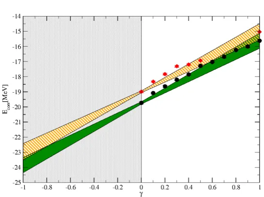
Figure 2.1: Extrapolations of CIMC correlation energies in the γ parameter for a system ofN =14 neutrons interacting trough chiral NNLOoptinteraction.

Black circles data were obtained using a Coupled–Cluster type wave–function with amplitudes calculated from PT2 while for the red diamonds we added a stochastic component to the amplitudes (cf. Eq.(2.23)).

∣M F⟩and we obtain the following recursive relation (see Appendix C for details)

ΦM_CCD(p1p2⋯pM

h1h2⋯hM) = ⟨m∣ΦCCD⟩ ≡ΦCCD(m)

=∑M

γ=2 M

∑

µ<ν

(−)γ+µ+ν_tpµpν

h1hγΦ

M−2 CCD(

p1p2⋯pµ−1pµ+1⋯pν−1pν+1⋯pM

h2⋯hγ−1hγ+1⋯hM ) ,

(2.21) .

In the above equation we assumed that the single–particle indices are or-dered, ie. p1 <. . .<pm andh1<. . .<hm. The wave function has a vanishing

component for odd M, and the component for M = 0 is fixed by our choice of normalization to be 1 (ie. ⟨ΦM F∣ΦCCD⟩ =1). Tough we have concentrated

just on the CCD case, it is clear that extensions to include singles (CCSD) and triples (CCSDT) corrections, useful for treating inhomogeneous systems or many–body interactions, are straightforward and we are actively working in this direction.

Amplitudes from many–body perturbation theory

As we just saw CC wave–functions are an excellent choice as trial wave–functions, however, solving the CC equations (2.20) is computationally expensive. There-fore, we investigated the possibility of using less computationally demanding ways of obtaining the tab

ij, while still preserving the structure of the CC wave

(27)

2.3. BASIS SET CONVERGENCE AND EXTRAPOLATIONS 19

perturbation theory (MP2):

tab_ij = ⟨ij∣∣ab⟩ ηi+ηj−ηa−ηb

with ηq =q+ ∑ k

⟨qk∣∣qk⟩. (2.22)

If the CC equations are solved iteratively, then this is equivalent to stopping after the first iteration. In this way we are able to obtain decent wave–functions in a fraction of the time even when the iterative solution shows difficulties in convergence (eg. when static correlations are important).

This choice for the amplitudes is clearly a worse approximation than using the fully–converged CCD amplitudes, however since we are using these wave– functions as constrain for the random walk, as long as the nodal structure is sufficiently well-described the particular form of ΦT should not matter since the

Monte Carlo walk will develop the missing correlations. We have tested in few selected cases that this is indeed true and moreover, provided we include the

γ–extrapolation step Eq.(2.14), the algorithm is so robust that we obtain reason-able values for the energy (within statistical error–bars) also by adding random noise to the amplitudes. For instance, in Fig.2.1 we show estimates of the CIMC correlation energies obtained at different values of the γ parameter (and cor-responding γ=0,1 extrapolation bands) for two different wave–functions: the black circles are obtained using amplitudes obtained from PT2 while for the red diamonds we used the distorted amplitudes

˜

tab_ij =tab_ij(0.5+ξ) (2.23) whereξis a random number uniformly distributed in[0,1]. Even with this crude approximation the extrapolated values (employing just γ=0 andγ =1) agree with each other. This is a clear signature that the sign structure is really encoded in the overall structure (ie. the exponential ansatz) of the wave–function and not in the precise values of the amplitudes. This opens a lot of opportunities when we will go beyond CCD by employing analogous approximate expressions for the singles and triplets.

2.3

Basis set convergence and extrapolations

Working in a big but finite basis set requires some careful study on the conver-gence of the calculations that we carry out. A direct, and costly, check for the convergence of a finite–basis calculation is simply to increase the basis size until results no longer change within a predetermined threshold. This is the proce-dure we adopted for all the neutron matter calculations ([66, 67, 68]) in Section 3.1, where the presence of regulators in the interactions effectively suppresses the importance of contributions from high–energy states. In other situations, like the Homogeneous Electron Gas [65] in section 2.4, the convergence may be problematic due to the slow decay of the matrix elements of the Coulomb potentials as a function of the momentum–transfer in particle collisions (cf. Eq.(2.26)).

(28)

300 400 500 600 700 800 q [MeV]

-2.5 -2 -1.5 -1 -0.5 0

Ecorr

[MeV] _-2 _-1.5 _-1 _-0.5 ₀

E_corr (PT2) [MeV] -1.5

-1 -0.5 0

Ecorr

(CIMC) [MeV]

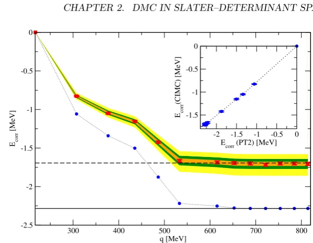
Figure 2.2: Plot of the correlation energy for N=14 neutrons obtained from PT2 (blue circles) and CIMC (red squares). The bands corresponds to extrapolations obtained fitting (2.25) up to Ω≡435 MeV (yellow band), Ω≡486 MeV (green band) and Ω≡652 MeV (orange band). The inset shows the CIMC correlation energy as a function of the PT2 correlation energy.

one can suppose that when the number of plane–waves Ω becomes large enough, the resulting energyE(Ω) ≈ (1/Ω)and one can extrapolate to the Ω→ ∞limit. Under this assumption of linearity one can even devise efficient schemes (see [69]) where a single calculation, performed at a value of Ω believed to be large enough, can be used to perform directly the calculations by estimating smaller– Ω results on–the fly.

Where exactly this linear regime starts is however a controversial question, in Section 2.4 we observe such trend just in the less interacting system considered. In this small section we want to report on a simple extrapolation method, based just on empirical evidence, that resulted to be quite robust against tests we did in many systems explored in our simulations.

The idea starts by noticing that the behavior of the correlation energy cal-culated with CIMC as a function of Ω is quite similar to the one produced by second order PT. As can be seen in Fig. 2.2 (where CIMC data are the red squares and PT2 results are the blue circles), we have approximately that

ECIM C_corr (Ω) ≈γEP T_corr2(Ω), (2.24) with a Ω–independent constant γ. If we now plotE_corrCIM C(Ω)as a function of

E_corrP T2(Ω)we find indeed a smooth behavior (see inset in Fig.2.2). In some cases, like HEG with rs≤ 1, a fit to the MC data with the simple ansatz Eq.(2.24)

(29)

2.4. APPLICATION: 3D HOMOGENEOUS ELECTRON GAS 21

additional, arbitrary, parameterη:

E_corrCIM C(Ω) ≈γE_corrP T2(Ω) +ηE_corrP T2(Ω)2 (2.25) to get a good fit withχ2_≈_{1. The three bands (orange, purple and green) in}

Fig.2.2 correspond to the results obtained using Eq.(2.25) when the two param-etersγandη are obtained trough fits to CIMC data up to the Ω corresponding to an UV cut-off of 435 MeV, 486 MeV and 652 MeV respectively. Values for higher momenta are predictions. In order to obtain the error bands we assumed

γandη to be perfectly correlated, thus the size of the bands may considered an upper–bound on the uncertainty (central values are much closer to the actual CIMC results).

It is striking to see that predictions made from the fit at values as low as 435 MeV, which is still far from the onset of the final plateau region, are capable of such accurate extrapolations with errors of≈8% in the correlation energy (<2% in energy per particle).

2.4

Application: 3D Homogeneous Electron Gas

As a first application we investigated the three dimensional homogeneous elec-tron gas (3DEG) using plane wave states, with definite momentum and spin as the sp basis set [65]. The 3DEG is described by a simple Hamiltonian; it never-theless encapsulates many of the difficulties associated with modern many-body theories. In particular, it has both the weakly and strongly correlated regimes which can be accessed via a single tunable density parameter, the Wigner-Seitz radiusrs, thus providing an ideal system for benchmarking many body theories

[29, 30, 69, 70, 71, 72].

The single–particle (sp) energies employed are εi =k2i/2m, where ki is the

momentum of thei-state, andmis the fermion mass. We include in our sp basis all single-particle statesiwith k_i2≤k2max. The interaction matrix elements are

given by:

V_ijab= (1−δka−ki,0)δki+kj,ka+kb

4π

Λ 1

(ka−ki)2

= (1−δka−ki,0)δki+kj,ka+kb

3

N

1

r3 s

1

(ka−ki)2

,

(2.26)

where the volume Λ=L3 _{of the simulation box (and hence the unit spacing in}

momentum) is determined by the density (orrs) and the number of particlesN.

We ignore the Madelung term because it does not affect the correlation energy. In Table 2.1 we show the CCD energies, calculated using conventional CC theory, along with the corresponding Monte Carlo energies of an 3DEG system with N =14 andNs=342, for rs=0.5,1.0 and 2.0. For these calculations we

used γ = 0 in expressions (2.11), (2.12) and (2.13). We see that, for rs =0.5

the CCD energy is very close to the corresponding Monte Carlo energy. But, for rs = 1.0 and 2.0 they are, in fact, lower than the corresponding Monte

Carlo energies. Since, ECIMC ≤ ⟨ΦCCD∣H∣ΦCCD⟩ (see discussion above), this

(30)

Correlation energy (a.u.)

rs CCD + CIMC CCD(PT2) + CIMC

0.5 −0.572682 −0.5729(3) −0.659641 −0.5733(2) 1.0 −0.506701 −0.5021(3) −0.657347 −0.5025(2) 2.0 −0.417946 −0.40317(2) −0.665071 −0.4029(3)

Table 2.1: Correlation energies for N = 14 and Ns = 342 from conventional

CC theory with the CCD and CCD(PT2) wave functions, along with the corre-sponding CIMC energies using each as importance functions. The numbers in parenthesis indicate statistical error in the last significant digit.

In Table 2.1 the energies obtained using the MP2 amplitudes are denoted by CCD(PT2). These CCD(PT2) amplitudes produce a worse approximation to the ground state wave function as compared to the full CCD amplitudes. Nevertheless, when used as importance functions in our CIMC algorithm, the final estimate for the ground state energy for both cases are very close. The statistical errors are comparable forrs=0.5 and 1.0. Forrs=2.0 they are about

an order of magnitude lower when the full CCD amplitudes are used.

The above observation is encouraging because it means that, as we men-tioned in the previous section, it may not be necessary to solve the full CC equations to get reasonable tab_ij amplitudes. Of course, we do not expect the CCD(PT2) amplitudes to be satisfactory for more strongly correlated systems. Still, even in those cases one can, presumably, use computationally inexpensive approximations to the full CC equations. For the rest of this work, all the CIMC results have been computed using the CCD(PT2) amplitudes.

In Fig. 2.3 we show the CIMC ground state energy estimates for N = 14 and rs = 0.5,1.0,2.0 and 3.0 for some of our large basis size calculations. In

Refs. [75, 72, 69] it was suggested that for the 3DEG it might be possible to extrapolate to theNs→ ∞ limit by exploiting a linear 1/Ns dependence of the

correlation energy for large but finite Ns. Although, for rs =0.5 andN = 14

such a linear trend in the correlation energy is visible, for the other values ofrs

shown in the figure, no such trend is evident.

Basis size-1

-0.58 -0.57 -0.56 -0.55

-0.51 -0.50 -0.49 -0.48

Correlation energy (a.u.)

162-1 342-1

2378-1 -0.41 -0.40 -0.39

2378-1 342-1 162-1 -0.33

-0.32

r

s = 0.5

r

s = 2.0

r

s= 1.0

r

s = 3.0

Figure 2.3: Correlation energies for N = 14 and rs = 0.5,1.0,2.0 and 3.0 as

(31)

2.4. APPLICATION: 3D HOMOGENEOUS ELECTRON GAS 23

The situation is similar for calculations we performed with N =32 and 54. Thus, at least up to our largest basis size Ns= 2378, we cannot safely do an

extrapolation toNs→ ∞with a reasonably lowχ2.

Correlation energy (a.u)

rs N CIMC Other

0.5 14 −0.5875(6) −0.5959(7)[69] 38 −1.809(4) −1.849(1)[69] 54 −2.354(2) −2.435(7)[69]

−2.387(2)[71] 1.0 14 −0.5114(5) −0.5316(4)[69]

38 −1.521(4) −1.590(1)[69] 54 −2.053(4) −2.124(3)[69]

−2.125(2)[71] 2.0 14 −0.4103(6) −0.444(1)[69] 38 −1.134(7) −1.225(2)[69] 3.0 14 −0.333(1)

Table 2.2: Correlation energies from CIMC with the CCD(PT2) importance function for differentrs and N and Ns =2378. For comparison we have also

included the results from Ref. [71] (basis set independent) and Ref. [69] (ex-trapolated using single point extrapolation fromNs=1850 forN=14 and from

Ns =922 for N = 38,54). The numbers in parenthesis indicate the statistical

error in each case.

In Table 2.2 we show the ground state energy of different rsand N for the

largestNs(=2378)calculated by us. For comparison, we also include the energy

estimates from Refs. [71] and [69]. The energies in Ref. [71] are calculated using the r-space diffusion Monte Carlo method with an importance function that included backflow correlation on top of the Slater-Jastrow wave function. These are strict energy upper bounds with a bias due to the fixed-node approximation. Nevertheless, they are believed to be highly accurate.

On the other hand, in Ref. [69] the energies are calculated in a finite CI like basis set (as in this work), using the Initiator Full Configuration Interaction Quantum Monte Carlo method (i-FCIQMC). TheNs→ ∞results are obtained

by using the so called single point extrapolation from much smaller values of

Nsthan ours. These finite-basis set results are already in good agreement with

the other calculations, capturing between 93% to 99% of the correlation energy. The energy upper bounds can be systematically improved by including higher order excitations (triples) in the CC wave function and by using larger basis sizes. Possibly, a much faster way to achieve basis set convergence is to use a finite basis renormalized Coulomb interaction [76].

(32)

FCIQMC ori-FCIQMC scale as the size the many body Hilbert space, i.e., they are exponential in the system size,N, and the basis size,Ns.

Computational time (cpu hours)

rs N Ns CIMC i-FCIQMC

0.5 14 1850 384(0.6) 200

1.0 14 1850 768(1.6) 2500

2.0 14 1850 768(8.8) 2500

2.0 38 922 4608(–) 16000

Table 2.3: Computational cost of our method (CIMC) compared with the i -FCIQMC method [69] for differentrs,N andNs. The numbers in parenthesis

for CIMC are timings with a more efficient recent code.

Our method, instead, provides strict energy upper bounds, the tightness of which can be systematically improved by improving the quality of the im-portance function. Importantly, the computational cost of our Monte Carlo algorithm nominally grows as N2_(N

s−N), for both computational time (per

Monte Carlo step) and memory requirements. Due to this polynomial scal-ing, we expect our method to be applicable to much larger systems than those manageable by conventional diagonalization methods or by (i-)FCIQMC. We see evidence of this in Table 2.3, where we compare computational time in our method with that in i-FCIQMC (especially using the more efficient recent ver-sion). The statistical error for the two methods are comparable in each case.

2.5

Pure observables

In this section we want to give the necessary details to computepure expectation– values (PE) for operators that are diagonal in the basis that we are working on. In section 1.2.1 we have already seen that DMC–like techniques provide in general amixed expectation–value(ME) (cf Eq.(1.27)) which, for observables that does not commute with the Hamiltonian ˆH, is in general different from the PE:

⟨O⟩M E =⟨

ΨI∣Oˆ∣Ψ0⟩

⟨ΨI∣Ψ0⟩

≠ ⟨Ψ0∣Oˆ∣Ψ0⟩

⟨Ψ0∣Ψ0⟩

= ⟨O⟩P E (2.27)

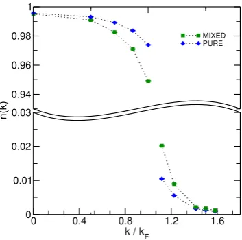
This is for instance the case if we want to calculate the occupation number operator,n(⃗k)in momentum–space org(⃗r)in coordinate–space. However, even in these cases, we can construct an estimator for the PE of the observable with the help of Hellmann–Feyman theorem.

Let us define an auxiliary hamiltonian ˆHO≡Hˆ+αOˆand the following energy:

Eτ(α) = ⟨

Ψτ∣HˆO∣Ψτ⟩

⟨Ψτ∣Ψτ⟩

=⟨ΨI∣HˆO∣Ψτ⟩

⟨ΨI∣Ψτ⟩

(2.28) where∣Ψτ⟩is the projected wave–function at imaginary–timeτ obtained using

the propagator corresponding to ˆHO:

(33)

2.5. PURE OBSERVABLES 25

.

Then the Hellmann–Feynmann theorem provides the following expression for the PE of ˆO:

⟨O⟩P E=lim α→0

∂E(α)

∂α (2.30)

where the derivative involved in the above equation can, in principle, be calcu-lated numerically. Numerical derivatives are however noisy, especially for small values ofαand we avoid this problem by using a recent algorithm developed in reference [77].

Let us first note that if ˆOis diagonal in the basis where we are working, the additional piece in the propagator

e−τ αOˆ

can be incorporated in thebranchingpart of the original propagator (cf. Eq.(2.5) and Appendix D), and thus simply amounts to a change in the weights of the configurations during the simulation. For instance the weight for a walker moving on the statenin a time–step ∆τ will now be given by:

b(n) Ð→bα(n) ≡b(α=0)(n)e−∆τ αOL(n). (2.31)

The total energy at imaginary–timeτwill be given by the (weighted) average among theNW walker present in the simulation1:

Eτ(α) =

∑NW

j bα(nτ;j)EL(α;nτ;j)

∑NW

j bα(nτ;j)

(2.32)

wherenτ;j is the Slater–Determinant occupied by thejth–walker at imaginary–

timeτ, whileEL(α;nτ;j)is the local–energy Eq.(1.17) calculated atnτ;j.

Walk-ers will accumulate corrections to the weight along the random walk so that the weight factorbα at timeτ will be given by:

bα(nτ) =b(α=0)(nτ)e− ∆τ α_∑τ

τ′OL(nτ′) _(2.33)

where the sum in τ′ goes in discrete steps ∆τ. The equation for the energy becomes then:

Eτ(α) =

∑NW

j b(α=0)(nτ;j)e−∆τ α∑

τ

τ′OL(nτ′;j)E_L(α;n_τ;j)

∑NW

j b(α=0)(nτ;j)e−∆τ α∑

τ

τ′OL(nτ′;j)

= ∑

NW

j b(α=0)(nτ;j)e−

Ground state and dynamical properties of many-body systems by non conventional Quantum Monte Carlo algorithms

UNIVERSIT `

Contents

Introduction and

Chapter 1

Introduction

1.1. INTRODUCTION 3

Projection Monte Carlo Algorithms

Diffusion Monte Carlo (DMC)

1.2. PROJECTION MONTE CARLO ALGORITHMS 5

1.2. PROJECTION MONTE CARLO ALGORITHMS 7

Ð→ ̃ODM C= ∑ M

1.2. PROJECTION MONTE CARLO ALGORITHMS 9

Reptation Monte Carlo (RMC)

1.2. PROJECTION MONTE CARLO ALGORITHMS 11

Chapter 2

Random walk on a Fock–space

2.2. IMPORTANCE–SAMPLING AND SIGN–PROBLEM 15

Importance–sampling and sign–problem

Coupled–Cluster wave–functions

2.2. IMPORTANCE–SAMPLING AND SIGN–PROBLEM 17

2.3. BASIS SET CONVERGENCE AND EXTRAPOLATIONS 19

Basis set convergence and extrapolations

2.4. APPLICATION: 3D HOMOGENEOUS ELECTRON GAS 21

Application: 3D Homogeneous Electron Gas

2.4. APPLICATION: 3D HOMOGENEOUS ELECTRON GAS 23

Pure observables

2.5. PURE OBSERVABLES 25