An Improved Method of Genetic Algorithm to Solve the Variable Speed Limit Problem with Constraint Conditions

(1)

An Improved Method of Genetic Algorithm to

Solve the Variable Speed Limit Problem with

Constraint Conditions

https://doi.org/10.3991/ijoe.v12i12.6448

Yishui Shui, Fang Li, Yichen Chen, Wei Chen

Wuhan University of Technology, Wuhan, China

Abstract—This paper analyses the genetic algorithm which is used to solve the problem of the variable speed limit (VSL) . In order to ensure the safety of driving, the speed limit in the chromosome must meet the constraints in time and space. The past practice is to add a penalty function in the object function, but with the increase of the number of solutions in the chromosomes, the weight of the penalty function is difficult to determine, often leads to the bad results. In this paper, we design a method to generate the chromosomes which meet the constraints, and the chromo-somes in crossover and mutation of the genetic algorithm still the meet the constraint conditions. By comparison, it is found that the method can converge faster than the penalty function method, and will generate an optimal solution under constraint conditions.

Index Terms—variable speed limit (VSL), safety, constraint condition, genetic algorithm, penalty function

I. INTRODUCTION

Genetic algorithm(GA)is founded by Holland of Uni-versity of Michigan[1].Based on the theory of population genetics and biological evolution, an optimization algo-rithm based on gene genetic and natural selection theory. Especially suitable for complex nonlinear constrained optimization problems which are difficult to be solved by traditional search methods. The algorithm is widely used in machine learning, combinatorial optimization, system engineering, adaptive control, artificial intelligence, plan-ning and design, intelligent manufacturing system, intelli-gent machine system, artificial life, etc [2].At present, genetic algorithm has become one of the effective meth-ods to study nonlinear phenomena and complex systems.

Variable speed limit is a very popular traffic control method in recent years. The specific implementation method is to use the traffic flow model and optimization algorithm to find a better speed limiting scheme, which can reduce the travel time, increase the traffic capacity, reduce the fuel consumption and pollution.Paper[3] uses VSL on a number of heavily trafficked freeway sections in Germany. Besides the impact on road safety, variable speed limits harmonize traffic flow at high volumes and hence influence freeway capacity. A.Hegyi in paper [4]use model predictive control to optimally coordinate variable speed limits and ramp metering. Allaby P, Hellinga B in paper[5] used a microscopic simulation model combined with a categorical crash potential model for estimating safety impacts. Paper[6] proposes a fuzzy control ap-proach for the traffic-responsive ramp metering and varia-ble speed limits control, in order to reduce the peak-hour

congestion on freeways. In paper[7],[8] resolve shock waves by dynamic speed limits with SPECIALIST algo-rithm. R Jiang, AB Lucky, E Chung[9] presents the results of a calibration and operational analysis of a candidate VSL algorithm for high flow conditions on an urban mo-torway of Queensland, Australia, speed-flow curve, travel time, speed deviation, fuel consumption and emission have been optimized all. Paper[10],[11] uses VSL to op-timize the traf!c control measures also reduce traffic emissions and fuel consumption due to increasing envi-ronmental concerns .The above papers use a variety of optimization algorithm to use variable speed to optimize the road section. It is proved that the method can improve the performance of freeway in many aspects. A control strategy is proposed in paper [12], including the speed limit, which must not exceed 20km/h in space and time. Paper[13],[14] also take the same control strategy with constraint conditions, and use the genetic algorithm to solve. But in the face of multiple solutions of these two papers have used the penalty function method. This paper find that use penalty function method of the genetic algo-rithm to solve the problem of VSL with constraint condi-tions is not ideal. So in this paper, an operator is designed which can produce chromosome conforms to the con-straint conditions. And on the basis of this design, the crossover operator and mutation operator are also design to achieve a diversified population. The simulation results show that the algorithm of this is effective, and has a big improve compare with penalty function method .

II. CONSTRAINT CONDITIONS CONFORM TRAFFIC

SAFETY

A. Modeling requirements

(2)

mapping from phenotype to genotype the encoding work. After the generation of initial population, according to the principle of survival of the fittest, generation by genera-tion evolugenera-tion produce better approximate solugenera-tion and in every generation. In each generation, according to the problem domain of individual fitness size selection indi-viduals, and with the genetic operators of crossover and mutation in nature genetics, represents a new solution set of the population. This process will lead to the kind of images of natural evolution of epigenetic generation pop-ulation than the previous generation more adapted to in the environment, best individuals of the last population after decoding can be as an approximation to the optimal solution.

Genetic algorithm is used to solve the VSL problem, when congestion occurs, use the simulation of traffic flow model to control the speed limit of different road sections at different time it can find the minimum total time spend (TTS).

In this paper, individual is the control speed and the population is the control speed set in time and space. In this paper as shown in the figure 1, the simulation section of the bottleneck and the occurrence of congestion, by controlling the speed of the upstream traffic flow to make less TTS. In this process upstream road needs to be seg-mented and time also need to be segseg-mented. This paper will divide the upstream 10km road into 10 sections which 1km a section, and 3 hours of simulation time is divided to 5 minutes a section and 36 sections in total, to form a matrix of 10 rows and 36 columns in Fig2. Speed on var-iable message signs(VMS) minimum 40km/h maximum 120km/h. And the speed can only be the value of integer times of 10, as is shown in formula 1.

; {40,50,60,70,80,90,100,110,120}

i

V A A! = (1)

!"##$%&%'(

!"#$%&'(

)*+$%*,-%*'. )"&*%+#,"&-./%/%

Figure 1. Schematic diagram of simulation road

1 2 3 10

Section

3hour v1(3h) v1(3h) v1(3h) … v1(10) bottleneck

… ! ! ! … ! bottleneck

(k+1)*5min v1(k+1) v2(k+1) v3(k+1) … v10(k+1) bottleneck k*5min v1(k) v2(k) v3(k) … v10(k) bottleneck 5min v1(1) v2(2) v3(3) … v10(10) bottleneck Time

bottle neck

Freeway

Figure 2. .Schematic diagram of the freeway sections and time

The speed and density difference of adjacent sections at the same time and also the same section of adjacent times should not be too large. If the gap is too large, first, will make the drivers frequentlyand greatly change their speed and lead to tired psychology. Second, different sections and different time period of speed and density difference is too large will make the traffic flow not smooth, result-ing in security issues. The study shows that the vehicle safety is the biggest threat to the vehicle speed difference.

Section !1(k+t) !2(k+t) … !i-1(k+t) !i(k+t) !i+1(k+t) … !N(k+t)

… … … … … … … …

!1(k+1) !2(k+1) … !i-1(k+1) !i(k+1) !i+1(k+1) … !N(k+1) !1(k) !2(k) … !i-1(k) !i(k) !i+1(k) … !N(k) Time

k+t k+1

k

1 2 i-1 i i+1 N

Figure 3. .Schematic diagram of the traffic density of freeway section and time

(

)

( )

max

0

#

!

i

k

+

1

"

!

i

k

# $

!

₍₂₎

( )

1

( )

max

0

#

!

i

k

"

!

i"

k

# $

!

₍₃₎

Section

v1(k+t) v2(k+t) … vi-1(k+t) vi(k+t) vi+1(k+t) … vN(k+t)

… … … … … … … …

v1(k+1) v2(k+1) … vi-1(k+1) vi(k+1) vi+1(k+1) … vN(k+1)

v1(k) v2(k) … vi-1(k) vi(k) vi+1(k) … vN(k)

Time k+t

k+1

k

1 2 i-1 i i+1 N

Figure 4. Schematic diagram of the traffic speed of freeway section and time

(

)

( )

max

0

"

v k

i

+

1

!

v k

i

" #

v

_{(4 )}

( )

1

( )

max

0

"

v k v

i ! i!

k

" #

v

₍₅₎

(

1

)

( )

_{( 1)}i k( )

i i _{i k}

v k

!

= ₊

+

!

(6)

( )

1 i k_{1( )}

i i _i _k

v

k v k

!

+ = ! ₊

(7) ! As the above Fig.3 and Fig.4 and formulas, at time k and section i the density and speed with the adjacent sec-tions i-1 and i+1 and the adjacent time period k-1 and k+1 velocity and density difference should not be too big. Also taking into account the proportion of the speed and densi-ty, so control the speed is equal to control the density. The calculation need to be as simple as possible, so define the speed difference of adjacent sections and times is 20km/h.

(

)

( )

0

"

v k

i

+

1

!

v k

i

"

20

₍₈₎

( )

1

( )

0

"

v k v

i ! i!

k

"

20

₍₉₎

( )

;

{40,50,60,70,80,90,100,110,120}

i

v k A A

!

=

₍₁₀₎

B. The constrained matrix generated to meet the

constraint conditions

First randomly generatedv1(1)

1(1) ; {40,50,60,70,80,90,100,110,120}

v !A A= ₍₁₁₎

Then randomly generatedv2(1)

1 1

2

{40,50,60,70,80,90,100,110,120} { (1) 20 (1) 20, 10 } (1) ;

A

B x v x v x N

v A B

=

= ! " " + # $

# % ₍₁₂₎

Then randomly generatedvi(1)

1 1

{40,50,60,70,80,90,100,110,120} { (1) 20 (1) 20, 10 } (1) ;

i i

i

A

B x v x v x N

v A B

! !

=

= ! " " + # $

# % ₍₁₃₎

(3)

1 1

1

{40,50,60,70,80,90,100,110,120} { (1) 20 (1) 20, 10 }

(2) ;

A

B x v x v x N

v A B

=

= ! " " + # $

# % ₍₁₄₎

Then randomly generatedv2(2)

1 1

1

{40,50,60,70,80,90,100,110,120}

{ (1) 20 (1) 20, 10 }

{ (2) 20 (2) 20, 10 }

(2) ;

A

B x v x v x N

C x v x v x N

v A B C

=

= ! " " + # $ = ! " " + # $

# % % ₍₁₅₎

So vi(k) conform to equations blow

1 1

{40,50,60,70,80,90,100,110,120} { ( ) 20 ( ) 20, 10 } { ( 1) 20 ( 1) 20, 10 }

( ) ;

i i

i A

B x v k x v k x N

C x v k x v k x N

v k A B C

! !

=

= ! " " + # $ = ! ! " " ! + # $

# % %

(16)

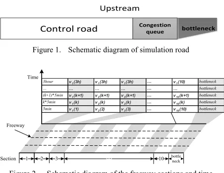
And generate a row in accordance with the constraint conditions of generating element. Finally generating ma-trix consistent with the constraints, as shown in Figure 5.

(a)

(b)

Figure 5. Simulation freeway sections and time pattern with and without constraint conditions

The matrix of the constraint conditions is represented by the color map and compared with the matrix without constraint conditions. Can be seen with the constraints of Fig.5(a) the matrix is more like contour map, the change is relatively smooth. And the matrix diagram that does not conform to the constraint conditions of Fig.5(b) is like the noise figure.

III. MUTATION AND CROSSOVER

This paper uses progressive generation method of gen-erating matrix consistent with the constraints, this matrix is the chromosome of the genetic algorithm. The combi-nation of the chromosome to form the initial population

participating in operation. However, crossover and muta-tion are needed to change the chromosome in genetic algorithm. So it is necessary to make the chromosome matrix in the crossover and mutation on the one hand to meet the rules of cross and mutation, but also on the other hand keep in line with constraints.

A. Mutation

A simple way to change the operation of a digital string is to change the number of digital. We start with the sim-plest encoding binary representation to illustrate, the bi-nary encoding means the position of each digital only has two possible 0 and 1 .

Figure 6. Schematic diagram of mutation

Its code length is 10 in Fig6, randomly generated a number K of 1 to 10 , if k=7,do the mutation operation to the right to the left of the seventh number and change it from 1 to 0 and get a new digital string.

In this paper, the mutation also uses the same operation. However, under the constraint conditions, the number of chromosomes in this paper can not randomly vary, be-cause if the random variation happened, the chromosome will not meet the constraints.

40 50 60

60 60 50

60 50 40

Figure 7. Mutation with constraint conditions

For example, number v ki( )_{in the middle of the fig7 is}

60, it can not change casually, but to meet the constraints of change.

1 1

{40,50,60,70,80,90,100,110,120}

{ ( ) 20 ( ) 20, 10 }

{ ( 1) 20 ( 1) 20, 10 }

{ ( ) 20 ( ) 20, 10 }

{ ( 1) 20 ( 1) 20, 10 }

( ) ;

i i

i

A

D x v k x v k x N

E x v k x v k x N

v k A B C D E

! !

+ +

=

= ! " " + # $

= ! ! " " ! + # $

= ! " " + # $

= + ! " " + + # $

# % % % %

(17)

In the above Fig.7,v ki( )_{according to its upper and} low-er, front and back numbersv ki( ) {40,50,60,70}! ,v ki( )_{can only}

change in this aggregate. The v ki( ) will not appear empty,

because the aggregate at least contains the original v ki( ). According to the above constraints equations, mutation in rows, the probability of 50% of the mutation in each row, each elements’ mutation according to the constraint condition.

The following figures are the matrixes before and after the mutation and the D-value of the two matrix, which can intuitively see the points of variation and the magnitude of the change.

0

5

10

15

20

25

30

35

40

0 2 4 6 8 10 40 50 60 70 80 90 100 110 120

0

5

10

15

20

25

30

35

40

(4)

(a)

(b)

Figure 8. The matrix patternbefore(a) and after(b) mutation

Figure 9. The matrix pattern of mutation points

B. Crossover

The simple way of crossover operation is to exchange the two individuals, P1 and P2 as their parents, to ex-change the value of the two parts of the code. Suppose there are ten bits long by two individuals.

!

Figure 10. Schematic diagram of crossover

Select a random position and length, such as position 7 length 2. Exchange the seventh and eighth elements of P1 P2 and to form a new chromosome P3 P4

Under the constraints of this paper, the crossover is also faced with the same problem when doing the mutation operation, which is not only to satisfy the exchange but also to satisfy the constraints. If only doing exchange elements as shown on the above, the elements of the ex-change and the elements around it must not be connected with the constraints. In this case, it is needed to change the new exchange elements to match the original chromosome to meet the conditions of exchange. So in this case, the crossover of this case will necessarily bring about muta-tion. We call the process of two matrices which are matching the constraint condition combine together by changing at boundary and combined into one matrix that meets the constraints called self matching.

The number of the crossover rows is 5.

v v v v v v v v v v

self matching…..

self matching…..

!

Figure 11. Schematic diagram of crossover with constraint conditions

After crossover, self matching is performed on the original matrix.

v1(k-1) v2(k-1) v3(k-1) v4(k-1) v5(k-1) v6(k-1) v7(k-1) v8(k-1) v1(k) v2(k) v3(k) v4(k) v5(k) v6(k) v7(k) v8(k) v1(k+1) v2(k+1) v3(k+1) v4(k+1) v5(k+1) v6(k+1) v7(k+1) v8(k+1)

Figure 12. Schematic diagram of crossover boundary

Gray rows in Fig.11 are foreign crossover rows, the white rows of lower part is from the original matrix. The foreign crossover rows and the original matrix line is in line with the constraints. However, the boundary line of the upper and lower does not meet the constraints. Change the original matrix elements, if the value of the original matrix elements meet the constraints remain the element unchanged, if not satisfied, change the element. By anal-ogy, a row is changed until the value of the row does not need to be changed, at this time, the cross line and the original matrix are all connected together in accordance with the constraints. The logical relation is

If

1 1

{ ( ) 20 ( ) 20, 10 } { ( 1) 20 ( 1) 20, 10 } ( )

i i

i

v k B C

! !

= ! " " + # $

= ! ! " " ! + # $

# %

(18)

( )

i

v k remain unchanged else

1 1

{40,50,60,70,80,90,100,110,120} { ( ) 20 ( ) 20, 10 } { ( 1) 20 ( 1) 20, 10 }

( ) ;

i i

i

A

v k A B C

! !

=

= ! " " + # $

= ! ! " " ! + # $

# % %

(19) 0

5

10

15

20

25

30

35

40₀ ₂ ₄ ₆ ₈ ₁₀ 40 50 60 70 80 90 100 110 120

0

5

10

15

20

25

30

35

40₀ ₂ ₄ ₆ ₈ ₁₀ 40 50 60 70 80 90 100 110 120

0

5

10

15

20

25

30

35

(5)

(a)

(b)

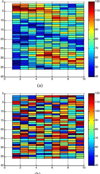
Figure 13. The first(a) and second(b) matrix pattern of difference before and after the crossover

The Fig.13(a) and Fig.13(b)are the two matrices of random exchange five rows and start the self matching mechanism and get a new matrix . Do the subtraction with the original matrix and get the matrix color chart. It can be seen that the boundary of the five rows is automatically matched with the original matrix. This method can be used for chromosome crossover in accordance with the constraint conditions.

IV. PENALTY FUNCTION METHOD

A. Fitness function

When using GAs to solve the optimization problem, the wayis to rely on the size of the fitness function value to distinguish the merits of each individual. Individuals with large fitness value will have more chances to reproduce the next generation in order to improve the average fitness of the population and the performance of the best individ-uals, the fitness function plays a decisive role in the GAs.

In order to solve the problem of constraint conditions ,the traditional method is to introduce the penalty function, and the constraint condition is transformed into penalty function. Then, integrate the penalty function and fitness function and GA will eliminate the individuals which are not satisfy the constraints. The specific process is as fol-lows:

(

)

( )

0

"

v k

i

+

1

!

v k

i

"

20

(20)

( )

1

( )

0

"

v k v

i ! i!

k

"

20

₍₂₁₎

First, the constraint conditions are transformed into standard constraints:

( )

(

)

( )

1

( ) 0; ( ) 20;

( ( )) 1 20

i i i i

i i

g v g v v k v k

g v k v k v k

! !

!

" = "

= + "

(22)

1 1

1 ( ) 1 ( ( ))

( )

.... ( ) 0

( ) 0... ( ) 0

n k

i

i k

j j g v k g v k

j

v

g v

v

g v

!

"

!

# #

= =

+

=

$

>

=

%

₍₂₃₎

TTS is the smaller the better,

!

j

( )

v

_{is the smaller the} better, but because the objective function is the greater the degree of higher adaptation, so the !j( )v _{plus TTS and}

then take the reciprocal, get the fitness function.

1

( )

j

fitness

=

TTS

+

!

v

(24)

It should be noted that, because of the number of solu-tions in chromosomes are too many, the actual punishment is difficult to determine.if the punishment is too large, the task of genetic algorithm become looking for the matrix to meet the constraints but not the smallest TTS. If punish-ment is too small, get the optimal solution in fact, not in line with constraint conditions .

In the setting of penalties, to make the penalty function and its corresponding objective function in the same mag-nitude.

B. Simulation analysis

Model construction

1. Bottleneck occurs in the 10km, the simulation of the total road is the upstream of the 10km road of the bottle-neck section.

2. VMS distance is 1km, the control time interval is 5min. Simulation time is 2 hours.

3. The maximum flow of bottleneck is 2000 vehicle / hour. During two hours of simulation time traffic flow is stable at 2500 vehicle/hour, the road sections appear seri-ous congestion.

4. Speed on VMS minimum 40km/h maximum 120km/h. And the speed can only be the value of integer times of 10km/h.

Select the same order of magnitude of the

!

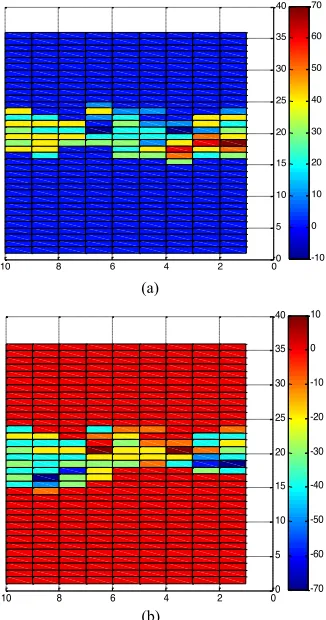
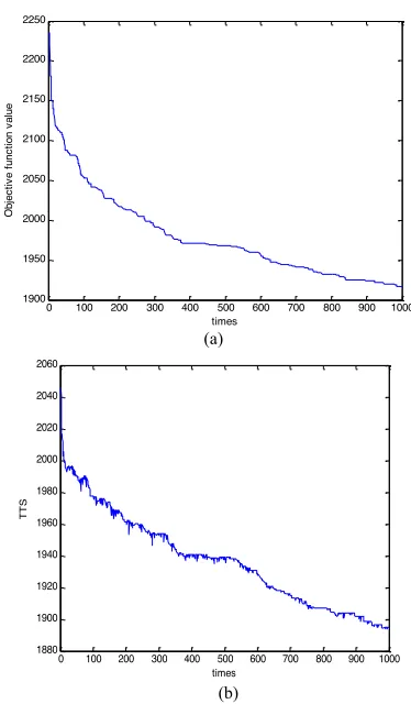
j( )v _with TTS to do the simulation. The TTS value is about 2000, the initial value of the objective function is 3820 in fig14(a), after 1000 times cycle optimization, the objective function value is reduced to 2160.Figure 14(b) is the change of the TTS in the 1000 cycle optimization, visible TTS has fluctuation, and the value change from 2035 to 2041. Thus, the penalty function method is useless, it looks only for conforms to the constraint matrix without looking for TTS, and slow convergence, after 1000 cycles did not find a matrix fully consistent with the consistent, at the same time, there is no optimization for TTS.

Make the coefficient

!

reduce to 1/10 of the value above. Genetic algorithm can do the normal operation for the main target TTS, but algorithm still can not find the matrix fully comply with the constraint conditions make the formula

!

j( )v _{sum zero. At the same timeFig.15(b)} compared with the following figure, the algorithm with 900 cycles to make the TTS to reach 1900, and the meth-od used in this paper to achieve TTS=1900 cycles only uses 50 times in Fig.16.

0 5 10 15 20 25 30 35 40

0 2 4 6 8

10 -10

0 10 20 30 40 50 60 70

0 5 10 15 20 25 30 35 40

0 2 4 6 8

10 -70

(6)

(a)

(b)

Figure 14. The first(a) and second(b) matrix pattern of difference before and after the crossover

(a)

(b)

Figure 15. The fitness function convergence curve

Figure 16. Thefitnessfunction convergence curve

And the method which is used to generate the constraint matrix has achieved a good result. Convergence rate is very fast, 200 times after the loop can get a good solution which TTS=1885 compared to the fixed speed limit of 120km/h, the total travel time decreased by 5.02%.Compared to the application of the method of pen-alty function, the method of this paper can not only meet the constraints, but also allows the genetic algorithm to find a shorter TTS with a faster speed.

V. SUMMARY AND DISCUSSIONS

This paper has developed a method to generate the re-stricted conditions of the limit speed matrix chromosomes before the calculation of genetic algorithm.And making crossover and mutation of the speed limit matrix chromo-somes are also in line with the constraints of the condi-tions in the process of the genetic algorithm.

The previous papers had used the penalty function method, but when road sections and time intervals in the simulation become more and more which leads the num-ber of solutions in the chromosome will also become more. In this case using the penalty function have not been able to solve the problem, no matter how to choose penal-ty function coefficient ,the calculation results are unac-ceptable. In contrast, the method of this paper can be a good solution to this problem.

In the production of matrix consistent with the con-straints, using line by line method to create the generation . The first number of the first row is randomly generated. And then, based on the first number and the constraints, the second number is generated. And then the third, fol-lowed by analogy, the numbers of the first row are gener-ated. The generation of the number in the second row of the first column is subject to constraints of the number of the first column and first row. Then each number is sub-ject to the previous number and the number above. Fol-lowed by analogy, the numbers of the matrix are generat-ed in this method.

Mutation is also required to implement under constraint conditions. Randomly select one row, do the mutation from the first column one by one to the last column. Every number of mutation has to be bound by the three numbers which are above it under it and before it.

Crossover can also be implemented under constraint conditions. But after crossing, on the edge of the crossed lines, some elements need to be changed to make the matrix in accordance with the constraints. The specific implementation method is to check the each number in the

0 100 200 300 400 500 600 700 800 900 1000 2000

2200 2400 2600 2800 3000 3200 3400 3600 3800 4000

times

O

bj

ec

tiv

e f

unc

tion v

al

ue

0 100 200 300 400 500 600 700 800 900 1000 2010

2020 2030 2040 2050 2060 2070 2080

times

TT

S

0 100 200 300 400 500 600 700 800 900 1000 1900

1950 2000 2050 2100 2150 2200 2250

times

O

bj

ec

tiv

e f

unc

tion v

al

ue

0 100 200 300 400 500 600 700 800 900 1000 1880

1900 1920 1940 1960 1980 2000 2020 2040 2060

times

TT

S

0 100 200 300 400 500 600 700 800 900 1000 1860

1880 1900 1920 1940 1960 1980 2000

times

TT

(7)

original matrix on the crossed boundary after the crosso-ver. If it satisfies the constraints of the crossover row, keep it unchanging, otherwise generatean new element, do the same job row by row until all the elements are in line with the requirements.

By comparing with the same simulation conditions, the method of this paper is much better than the penalty func-tion method. When the penalty funcfunc-tion method chooses the same order of magnitude of

!

j( )v _{the genetic algorithm} is used to search for the constraint matrix instead of the shorter TTS. When choosing a decimal order of magni-tude of!j( )v after a very long cycle it could not find a

ma-trix completely conforms to the constraint, and also the optimize speed of TTS is very slow. Penalty function method has a very big performance gap compared with the method this paper used.

REFERENCES

[1] Holland J H. Adaptation in natural and artificial systems[M]. MIT Press, 1992.

[2] Yao X, Xu Y. Recent Advances in Evolutionary Computation[J]. Journal of Computer Science & Technology, 2006, 21(1):1-18.

https://doi.org/10.1007/s11390-006-0001-4

[3] Geistefeldt J. Capacity effects of variable speed limits on German freeways[J]. Procedia - Social and Behavioral Sciences, 2011, 16(1):48-56. https://doi.org/10.1016/j.sbspro.2011.04.428

[4] Hegyi A, Schutter B D, Hellendoorn H. Model predictive control for optimal coordination of ramp metering and variable speed lim-its[J]. Transportation Research Part C Emerging Technologies, 2005, 13(3):185-209. https://doi.org/10.1016/j.trc.2004.08.001

[5] Allaby P, Hellinga B, Bullock M. Variable Speed Limits: Safety and Operational Impacts of a Candidate Control Strategy for Freeway Applications[J]. IEEE Transactions on Intelligent Trans-portation Systems, 2008, 8(4):671-680. https://doi.org/10.1109/ TITS.2007.908562

[6] Ghods A H, Kian A, Tabibi M. A genetic-fuzzy control applica-tion to ramp metering and variable speed limit control.[C]// Sys-tems, Man and Cybernetics, 2007. ISIC. IEEE International Con-ference on. IEEE, 2007:1723-1728.

[7] Schelling I, Hegyi A, Hoogendoorn S P. SPECIALIST-RM — Integrated variable speed limit control and ramp metering based on shock wave theory[C]// Intelligent Transportation Systems (ITSC), 2011 14th International IEEE Conference on. IEEE, 2011:2154-2159.

[8] Hegyi A, Hoogendoorn S P, Schreuder M, et al. The Expected Effectivity of the Dynamic Speed Limit Algorithm SPECIALIST: A Field Data Evaluation Method[J]. Civil Engineering & Geosci-ences, 2009:1770-1775.

[9] Jiang R, Lucky A B, Chung E. Calibration and operational analy-sis of Variable Speed Limits for high flow conditions[C]// Inte-grated and Sustainable Transportation System (FISTS), 2011 IEEE Forum on. IEEE, 2011:221-226.

[10] Zegeye S K, De Schutter B, Hellendoorn J, et al. Variable speed limits for green mobility[C]// Conference Record - IEEE Confer-ence on Intelligent Transportation Systems. 2011:2174-2179.

https://doi.org/10.1109/itsc.2011.6082833

[11] Liu B, Ghosal D, Chuah C N, et al. Reducing Greenhouse Effects via Fuel Consumption-Aware Variable Speed Limit (FC-VSL)[J]. IEEE Transactions on Vehicular Technology, 2012, 61(1):111-122. https://doi.org/10.1109/TVT.2011.2170595

[12] Carlson R C, Papamichail I, Papageorgiou M. Local Feed-back-Based Mainstream Traffic Flow Control on Motorways Us-ing Variable Speed Limits[J]. IEEE Transactions on Intelligent Transportation Systems, 2012, 12(4):1261-1276.

https://doi.org/10.1109/TITS.2011.2156792

[13] HongmeiLIANG.Research on Multi-Objective Optimization and Decision-Making Method of Variable Speed-Limit Control for Freeways.(Master Thesis) Jilin University, Changchun, Jilin,China 2015

[14] Ping WANG.Research On The Variable Speed Limit Method of The Topical Rainfall Segment On Freeway(Master Thesis) Wuhan University of Technology, Wuhan, Hubei, China.2012

AUTHORS

SHUI Yishui received the B.S and M.S degree in communication engineering from Wuhan University of Technology Wuhan, China in 2010 and 2013. Now he is pursuing the Ph.D. degree at Wuhan University of Technology, 430070, Luoshi road No. 122. His research interest includes the Intelligent Transportation and Intelligence Algorithm ([email protected] or [email protected]).

LI Fang received the B.S. degree in communication engineering from Wuhan University of Technology, Wu-han, China, in 2010 and the M.S. degree in Communica-tion and InformaCommunica-tion System engineering from Wuhan University of Technology, Wuhan, China, in 2013. She is currently pursuing the Ph.D. degree in Traffic control and information engineering at Wuhan University of Tech-nology, Wuhan, China ([email protected]).

CHEN Yichen received the bachelor's degree in elec-tronic in-formation engineering from Wuhan Textile Uni-versity, Hubei, Wuhan, in 2014 . She is currently pursuing the master's degree in information and telecommunication engineering at Wuhan University of Technology. Her research interest includes the Intelligent Transport System and vehicle networking ([email protected] ).

CHEN Wei received the Ph.D. degree in information and communication engineering from the Huazhong Uni-versity of Science and Technology, Wuhan, China, in 2005.He is currently a Professor and a Doctoral Supervi-sor with the School of Information Engineering, Wuhan University of Technology. His current research interests include intelligent traffic control systems ([email protected]).