unit4 CHETN XIII 3 Briggs Modeling Sep13

Basics of Physical Modeling In Coastal and

Hydraulic Engineering

ARTICLE · SEPTEMBER 2013

DOWNLOADS 618

VIEWS 680

1 AUTHOR:

Michael J. Briggs Briggs Group, LLC

131PUBLICATIONS 615CITATIONS

Basics of Physical Modeling in Coastal

and Hydraulic Engineering

by Michael J. Briggs

PURPOSE: This Coastal and Hydraulics Engineering Technical Note (CHETN) presents a brief overview of the basics of physical or laboratory modeling. Since the Coastal and Hydraulics Laboratory (CHL) is primarily concerned with inland and coastal flooding and navigation issues, the scope of this CHETN is limited to physical modeling topics that are used in free-surface fluid flow problems.

BACKGROUND: The mission of CHL is to understand better the effects of water levels, tides, waves, and currents on coastal structures such as beaches, inlets, harbors, jetties, and breakwaters and riverine structures such as spillways, levees, locks, and stilling basins. Combinations of analytical, numerical, and laboratory modeling tools are typically used to ensure optimal designs. Physical models are an important component of the CHL mission. They are engineering tools that are used to (a) improve understanding and gain insight into the physics of coastal and riverine processes, (b) test and optimize proposed designs, and (c) provide data sets for improving numerical models. Physical systems that are reproduced in the model follow similarity laws derived from dimensional analysis so that the model accurately represents the prototype. In general, the ratio of like quantities should be the same in both the model and prototype.

Use of physical models is a well established engineering practice, especially in hydraulics and the design of ships (Hughes 1993; Chakrabarti 1994). William Froude (1810-1879) and Osbourne Reynolds (1842-1912) are among the most famous researchers relative to our branch of hydraulics. Froude studied the resistance of ships in a towing tank in 1870, which involved inertial and gravitational forces. Reynolds, a British engineer, developed the Reynolds number in his study of flow in parallel pipes to distinguish between laminar and turbulent flow conditions. The Froude and Reynolds numbers are two of the most important non-dimensional similarity parameters used in physical modeling. The CHL has been actively involved with physical modeling since its founding in 1929 to study the Mississippi River floods.

This CHETN discusses types of physical models in coastal engineering, hydraulic similitude and scale factors, Froude and Reynolds numbers, Froude-derived model scale factors for commonly used quantities, advantages and disadvantages of physical models, and design and planning of model experiments.

Coastal vs. Inland Models. Coastal models deal with processes that occur along coastlines. These include the effects of water levels, tides, waves, currents, and winds on beaches, islands, harbors, and coastal structures. Figure 1 is an example of a coastal model to study the flooding and levee failure in New Orleans due to Hurricane Katrina. Of course, Lake Ponchatrain is not on a coast, but is an interior lake. Large lakes such as Lake Ponchatrain and the Great Lakes are usually considered as coastal models since the main driving mechanism is waves. Inland models are concerned with the design and interaction of water flow in rivers, lakes, and streams with dams, locks, stream beds, and control structures. Figure 2 is an example of an inland model of The Dalles spillway that was used to optimize proposed design modifications.

Figure 1. New Orleans 17th Street Canal: coastal, fixed-bed, 3D, site-specific, 1:50 scale model to study flooding and failure of levees due to Hurricane Katrina (Source: Bill Seabergh).

Figure 2. The Dalles spillway: inland, fixed-bed, 3D, site-specific, 1:80 model scale to study design of spillway (Source: Glenn Davis).

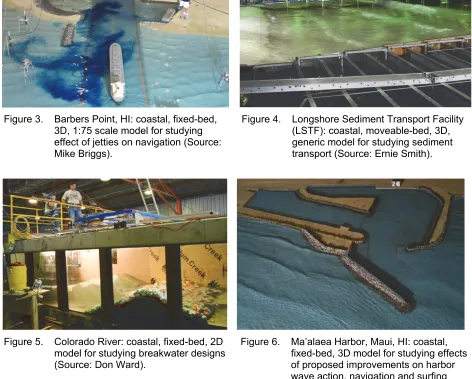
Fixed- vs. Moveable-Bed Models. Fixed-bed models have solid boundaries (e.g., cement) that are not modified by the hydrodynamic processes being modeled. This is the most common type of model and the scaling effects are relatively well understood. Figure 3 is an example of a fixed-bed model to optimize the jetty design and channel entrance at Barbers Point, HI. Moveable-bed models, on the other hand, have soft boundaries that interact with the hydrodynamic processes. They are used to study sediment transport issues such as beach profile evolution, dune erosion, scour around bottom-founded coastal structures, and changes in bathymetry due to water flow. The scaling for moveable-bed models is not as well understood as fixed models. Figure 4 is an example of a moveable-bed model for the Longshore Sediment Transport Facility (LSTF) for studying sediment transport issues using sand.

Figure 3. Barbers Point, HI: coastal, fixed-bed, 3D, 1:75 scale model for studying effect of jetties on navigation (Source: Mike Briggs).

Figure 4. Longshore Sediment Transport Facility (LSTF): coastal, moveable-bed, 3D, generic model for studying sediment transport (Source: Ernie Smith).

Figure 5. Colorado River: coastal, fixed-bed, 2D model for studying breakwater designs (Source: Don Ward).

Figure 6. Ma’alaea Harbor, Maui, HI: coastal, fixed-bed, 3D model for studying effects of proposed improvements on harbor wave action, navigation and surfing conditions (Source: Ray Bottin).

Site-specific vs. Generic Models. Site-specific models are designed for a particular prototype site with corresponding forcing conditions. They are used to verify and validate design(s) for that specific site only. Most of the figures already presented were of site-specific models. Generic models are usually simplified and idealized models intended to provide guidance for a variety of hydrodynamic processes. They can be used to investigate a particular response under controlled conditions, calibrate numerical models, or develop empirical relationships. Most generic models are patterned after a reasonable real world location, however. Figure 9 is an example of a generic model to study tsunami wave runup due to edge waves traveling around an island.

HYDRAULIC SIMILITUDE: The purpose of hydraulic similitude is to ensure that the model reproduces the behavior of the prototype as much as possible (Goda 1985; Hughes 1993; Young et al. 1997). This similar behavior includes velocity, acceleration, mass transport, and resultant fluid forces on objects and boundaries. Correspondence between prototype (p) and model (m) is denoted by the scale factor or model scale (NX), which is the ratio of the prototype parameter (Xp)

to the model parameter (Xm) defined as

 p

X m X N

X (1)

Note that one can sometimes see the inverse of this factor used to represent the scale factor (i.e., model divided by prototype value). This makes the scale factor look like a fraction less than one, as in 1 model-100 prototype. In this CHETN, the form given in Equation 1, where the prototype value is divided by the model value, is preferred. This X parameter can represent any derived variable as determined from its dimensions. For instance, fluid velocity (V) has dimensions of length (L) divided by time (t), so the velocity scale (NV) is given by









/ /

p p p m L

V

m m m p t

L t

V L t N

N

V L t L t N

 

 

  _{  } 

   (2)

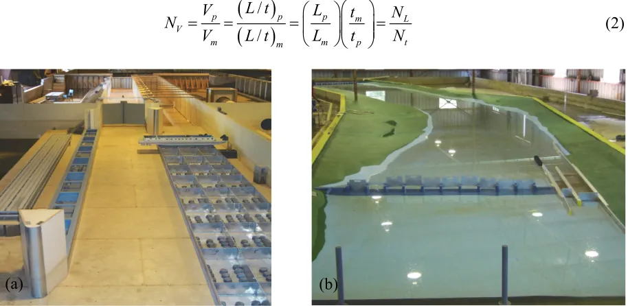
Figure 7. Inland, fixed-bed, 3D undistorted models for studying lock and dam operations: (a) J.T. Myers locks and dam and (b) Montgomery Lock on the Ohio River (Source: Howard Park).

Figure 8. Fixed-bed, 3D distorted models of (a) Los Angeles-Long Beach Harbors (LALB): coastal model for studying long-wave harmonics (Source: Bill Seabergh) and (b) Knik Arm, AK: inland model for studying unsteady, non-uniform current flows (Source: Steve Hughes).

Figure 9. Tsunami wave runup: coastal, fixed-bed, generic, 3D model for studying runup of edge waves on back side of island (Source: Mike Briggs).

The three basic laws of similitude are geometric (similarity of form), kinematic (similarity of motion), and dynamic (similarity of forces). In general, the ratio of quantities in the model needs to be the same as in the prototype. For geometric similarity, the ratio of model and prototype lengths must be equal. For kinematic similarity, velocity and acceleration must have the same ratios between model and prototype. For dynamic similarity, the four external forces of gravity (Fg), viscosity (Fv), surface tension (Fs), and elasticity (Fe) must have the same ratios. This

requirement arises from Newton’s Second Law which states that the inertial force (FI=ma)

equals the sum of these external forces.

In general, almost any modeling situation can be simplified as the interplay between two major forces as the other forces play a minor role. In fluid flow modeling, inertial forces are always present. The ratio of the inertial force to the other forces has led to the development of the similitude criterion that relates the importance of these secondary forces to the inertial force. No fluid can satisfy all the dynamic similarity requirements. Since the same fluid (i.e., water) is usually used for both model and prototype, it is impossible to achieve exact dynamic similarity for water waves. Surface tension and compressibility are generally neglected as they are relatively small. Viscosity can be neglected in most free-surface models if the model is not too

small. Thus, the Froude Number (defined below) is the major scaling criterion in coastal and inland models with free-surface flows.

Froude Model Law. The Froude number (Fr) is defined as the square root of the ratio of the

inertial force (force due to convective acceleration of a fluid particle) to the gravitational force (weight) as given by (Hughes 1993; Young et al. 1997):

2 2 I 3 g F F r

L V V

F

L g gL

 

   (3)

Froude similitude between model and prototype requires that the Froude numbers are equal:

r m p V V F gL gL     _ _ _ _

    (4)

Rearranging and expressing in terms of scale ratios (NX) of individual variables gives

p p p

V g L

m m m

V g L

N N N

V g L

   (5)

Reynolds Model Law. The Reynolds number (Re) is important when viscous forces dominate,

such as laminar boundary layer problems in open-channel or free-surface flows and forces on cylinders in low Re flows. Bottom friction can be significant if the flow depth is relatively small.

One way to minimize the influence of viscosity is to ensure that the model flow is in the turbulent range, which occurs for Re above approximately 104. The Reynolds number (Re) is

defined as the ratio of inertial to viscous forces (Hughes 1993; Young et al. 1997):

2 2 I v F F e

L V VL VL

R

VL

 

  

    (6)

where ρis the mass density, μ = dynamic viscosity, and ν (=ρ/μ) is the kinematic viscosity. As done with the Froude number, similitude is achieved when Reynolds numbers are equal in model and prototype:

e

m p

LV LV

R  

 

   

_{ } _{ }

    (7)

p p p p

V L

m m m m

V L

N N N N

V L            _{   }

    (8)

centrifuge or goes into space to alter gravity since there is no fluid that has a viscosity that can satisfy these constraints. In general, the Reynolds number can be neglected if it is greater than 104 and in the same range in model and prototype, even though they are not exactly the same.

Other Dimensionless Parameters. In addition to the Froude and Reynolds numbers, there are several other dimensionless numbers that can be derived for use in physical models (Young et al. 1997). These include (a) the Weber Number (We

)

tension, (b) the Cauchy Number (Ca

)

waves, impact forces, and mooring lines, and (c) the Strouhal Number (St) for the study of

acceleration effects in unsteady, oscillating flows, and vortices.

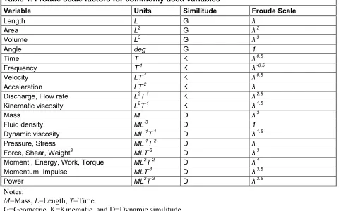
Froude-Derived Scale Factors. Table 1 lists Froude-derived scale factors for some common variables used in coastal and hydraulic engineering models (Goda 1985; Chakrabarti 1994). It includes units, type of similitude, and Froude-scaling relative to the model scale factor (λ). Note that λ is usually chosen based on the geometric similitude factor (NL) for characteristic lengths.

Also, it is assumed that gravity remains constant and fresh water is used in both model and prototype.

Table 1. Froude scale factors for commonly used variables

Variable Units Similitude Froude Scale

Length L G λ

Area L2 _{G λ}2

Volume L3 _{G λ}3

Angle deg G 1

Time T K λ0.5

Frequency T-1 K λ-0.5

Velocity LT-1 K λ0.5

Acceleration LT-2 K λ

Discharge, Flow rate L3T-1 K λ2.5

Kinematic viscosity L2T-1 K λ1.5

Mass M D λ3

Fluid density ML-3 _{D 1}

Dynamic viscosity ML-1_T-1 _{D λ}1.5

Pressure, Stress ML-1_T-2 _{D λ}

Force, Shear, Weight3 _MLT-2 _{D λ}3

Moment , Energy, Work, Torque ML2T-2 D λ4

Momentum, Impulse MLT-1 D λ3.5

Power ML2T-3 D λ3.5

Notes:

M=Mass, L=Length, T=Time.

G=Geometric, K=Kinematic, and D=Dynamic similitude.

Some criteria for the selection of the model scale factor are listed as follows:

 Make the model as large as possible since the larger the model, the more accurate the results as the model behavior is most like the prototype.

 Compromise on size if necessary as larger models cost more and may require more time to complete an experiment.

 Consider the size and availability of test facilities.

 Maximize model dimensions and sizes of measured quantities to minimize viscosity and surface tension effects.

There is no definite criterion for acceptable ranges of scale factors. However, most hydraulic laboratories have had success with scales in the range of 10 to 150 depending on the parameters tested (Dalrymple 1985; Hughes 1993; Chakrabarti 1994). The smaller values are usually in 2D models to minimize the scaling effects in studies involving structural details such as breakwater armor units.

ADVANTAGES AND DISADVANTAGES OF PHYSICAL MODELS: Some advantages

and applications of why physical models are important are listed as follows (Goda 1985; Hughes 1993; Chakrabarti 1994):

 Physical phenomena are often highly nonlinear and not well understood. Physical models usually replicate the physics, both linear and nonlinear, of physical processes very well, without simplifying assumptions.

 Physical models are used to determine empirical coefficients for analytical and numerical models that are not known or only poorly understood.

 Physical models assist in evaluating the effect of simplifying assumptions (i.e., discarding higher order terms) on numerical model predictions.

 Field experiments are very expensive and forcing conditions (i.e., waves, winds, water levels, currents) are difficult to control and systematically vary.

 Models provide repeatability and a controlled environment for calibrating analytical and numerical models. The smaller size permits easier and less expensive data collection of multiple variables such as water levels, pressures, forces, velocities, displacements, etc.

 Physical models provide a hands on look at the processes, allowing one to examine different options relatively conveniently and gain insight (qualitative impression) of the physics governing a process. In spite of the improved graphics of numerical models, most people can relate to the visual feedback and ability to interact with a physical model.

 Prototype construction may be very risky or uneconomical without a model to verify assumptions and performance. This is especially true the greater the cost and complexity of a project. In this case, a physical model study may be justified from the standpoint of verifying the prototype design and validating numerical model results.

The four main disadvantages of physical models (Hughes 1993; Chakrabarti 1994) can be listed as follows:

 Scale effects are due to the fact that it is impossible to correctly scale a free-surface hydrodynamic model using water that satisfies all of the laws of similitude. To minimize scale effects, one should construct as large a model as possible that fits within time, cost, and available facility space constraints.

 Laboratory effects consisting of model boundaries, instrumentation support, mechanical wave and flow generation losses, etc., are a concern in physical models. In the model, walls are necessary to contain the water, but they induce laboratory effects due to reflection and flow restriction. In the real world, there are no artificial boundaries to produce these effects. In the model, instruments are typically mounted in some type of rigid support that may have a larger impact on the flow field than a similar instrumentation support in the prototype. However, measures can be incorporated in the model to minimize and mitigate these effects. The generation of waves and currents by mechanical means in a laboratory is not exact between model and prototype. In the real world, waves may have multidirectional characteristics with frequency and directional spreading that are not always possible to simulate as accurately in the laboratory.

 Forcing functions or boundaries in the prototype may not be simulated in the model due to cost and/or practicality. For instance, simulating wind blowing across the surface is rarely included in coastal models. Instead, the wind effect is represented by the equivalent wave conditions at the wavemaker or wind effects on the model (i.e., ship heeling due to wind).

 Construction and application of a physical model may not be cost-effective. For relatively straightforward applications, numerical models can be more cost efficient. One must realize that numerical models also have limitations and simplifying assumptions that may significantly affect the results. Tradeoffs between physical and numerical model applications should be considered.

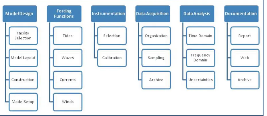
Figure 10. Planning a physical model.

SUMMARY: The purpose of this CHETN is to provide an overview of some of the basics of physical modeling as applied to coastal and inland hydraulic engineering within USACE. Different ways to classify physical models including fixed- versus moveable-bed, two- versus three-dimensional, and site-specific versus generic models are described. The basics of hydraulic similitude and scale factors including derivation of Froude and Reynolds numbers and other dimensionless factors used in fluid flow problems are discussed. The selection of model scale factors and calculation of equivalent model and prototype scaled values for commonly used quantities are described. The advantages and disadvantages of physical models are discussed including consideration of laboratory and scale effects. Finally, the steps involved in the design and planning of physical models from start to finish are presented.

POINTS OF CONTACT: This CHETN is a product of the Navigation Systems (NavSys) and the Flood and Coastal Storm Damage Reduction Research Programs at the US Army Engineer Research and Development Center, Coastal and Hydraulics Laboratory. Questions about this technical note can be addressed to Dr. Michael J. Briggs (Voice: 2005; Fax: 601-634-3433; e-mail: [email protected]). For information about the Navigation Systems Research Program (NavSys), contact the Program Manager, Eddie Wiggins at 601-634-2471; e-mail: [email protected]. For information about the Flood and Coastal Research Program, contact the Program Manager, Dr. Cary A. Talbot, at 601-634-2625; e-mail:

[email protected].This CHETN should be cited as follows:

REFERENCES

Chakrabarti, S. K. 1994. Offshore structure modeling. Advanced series on ocean engineering. Volume 9. Singapore and River Edge, NJ: World Scientific.

Dalrymple, R. A. 1985. Introduction to physical models in coastal engineering. In Physical Modeling in Coastal Engineering, ed. R. A. Dalrymple, pp. 3-9. Rotterdam, The Netherlands: A. A. Balkema.

Goda, Y. 1985. Random sea and design of maritime structures. University of Tokyo Press.

Hughes, S. A. 1993. Physical models and laboratory techniques in coastal engineering. Advanced series on ocean engineering . Volume 7. Singapore and River Edge, NJ: World Scientific.

Young, D. F., B. R. Munson, and T. H. Okiishi. 1997. A brief introduction to fluid mechanics. Hoboken, NJ: John Wiley and Sons, Inc.

NOTE: The contents of this technical note are not to be used for advertising, publication, or promotional purposes. Citation of trade names does not constitute an official