The Impact of Seasonality on the Implementation of Value at Risk (VaR) Models for
Predicting Future Non Profit Loans (NPL) Values in Albania
Eris Zeqo
“Aleksandër Moisiu” University of Durrës, Faculty of Information Technology, Albania Email: [email protected]
Ass.Prof. Lindita Mukli
“Aleksandër Moisiu” University of Durrës, Faculty of Information Technology, Albania Email: [email protected]
Dr. Jona Mulliri
Agricultural University of Tirana, Economy and Agribussines Faculty, Albania Email: [email protected]
Doi:10.5901/ajis.2016.v5n3s1p579
Abstract
One of the main problems in the Albanian financial market is the high rates of Non Profit Loans. As part of this problem, banks need to predict and calculate the level of reserve funds (provisions) to cover the possible losses from these loans. Currently these calculations are made based on the standard method which does not take in consideration many factors, including seasonality. The objective of this paper is to study if there is seasonality in the variance of NPL values for Albanian market. It is part of a study in relation to the possibility for the use of Value at Risk (VaR) models to predict future values of Non Profit Loans (NPL) in Albania. Using the official data from the Bank of Albania we first study the NPL time series by creating an initial predicting VaR model of future NPL values. Then the data are grouped under 3 months intervals and are studied to see if they have seasonality and if the existence of seasonality can improve the initial model.
Keywords: Value at Risk (VaR) models, Non Profit Loans (NPL), seasonality, Credit Risk, Internal Rating Based (IRB) Models.
1. Introduction
As a result of the global financial crisis, the regulations of financial institutions were changed to improve and to avoid the repetition of scenarios where losses of financial institutions were paid by governments (taxpayers).
One of the highlights of these regulations is the minimal level of capital a bank must hold to cover potential losses as a result of exposure to various types of risks. Central banks, as the supervisor authority, define the models to be used by commercial banks for the calculation of the level of regulatory capital that these banks should have. Usually standard methods imposed by the central banks have a conservative tendency that requires from commercial banks to hold a significant amount of capital to cover potential losses from their financial activity. Meanwhile, the desire of commercial banks is to hold less capital and to maximize the amount of business that they can perform.
The possibility to use personalized valuation methods, different from traditional methods, was introduced for the first time in the June 2004 as part of Basel II recommendations. Normally, these methods must be evaluated and approved in advance by the supervisor authority. Although these methods are introduced for more than a decade, in Albania the relevant legislation does not allow their use by commercial banks. For this reason, at the moment the use of an internal model can be limited as complementary and not as a substitute of the traditional model.
2. Standard Method limitations
Credit risk is the most difficult to manage because of the many dynamic factors that influence this risk. Not taking into account the numerous dynamic factors that influence the credit market is the main source of problems deriving from the standard method. Based on Basel regulations, there are two classifications for the models used to calculate the capital needed to cover the credit risk exposure:
• Standard method. Banks evaluate their risk exposure using outside estimates (ratings). All exposures are assigned to a specific risk group. This method specifies the capital required for each risk group. The standard method has its basis from Basel I, but is more detailed on Basel II and Basel III.
• Internal rating based (IRB) methods. Banks rely on their internal evaluations of some (basic IRB) or all (advanced IRB) risk components. These components are the probability of default, lost given default, exposure at default and effective maturity.
Currently in Albania the classification of loans and the rates for calculating provisions for each main category are based on the rules of the Bank of Albania. Loans are divided in 5 risk groups based on the period of delay in payment by the borrower where the last 3 groups form the NPL. Subject to the above categories and norms, banks create reserve funds to cover potential credit losses. As mentioned above, there are numerous factors that influence credit risk and are not reflected in the standard method:
• Invariance to credit portfolios, it does not reflect the importance of risk diversification or risk concentration as a key factor in portfolio's risk.
• Does not takes into account specific local risks.
• Traditional methods do not consider the fact that different types of risk affect each other, creating the possibility of "double counting" or not penalizing concentration risk.
• Limited classification of credit types, all loans classified in the same group are "penalized" equally, regardless of:
- the loan size - the maturity - the borrowers quality
These limitations of the standard methods are recognized even from the Basel Committee on Banking Supervision. First on 27 March 2015 and later on December 2015 they published two consultative documents for the "Revisions to the Standardized Approach for credit risk".
As part of the limited classification problem, seasonality in a factor to take into consideration when trying to implement IRB models.
3. Methodology
The objective of this paper is to make a quantitative research. We use the official time series data offered from the Bank of Albania on credit portfolio quality. The unit used for this data is in percentage. The study of these time series will be made for the July 2001 - March 2016 period and values will be divided into 3-month periods (quarters). Values before July 2001 are not taken into consideration because earlier periods are influenced by the unusual economic situation caused after the collapse of financial institutions in Albania in 1997. The NPL values in the period October 1998 - June 2001 were at the level of 33.4% - 55.1% while in the third quarter of 2001 they went down by 29% reaching a value of 11.2%.
The study of seasonality on the variance of NPL values is part of a research regarding the possibility to use Value at Risk models as IRB models for calculating the level of regulatory capital that commercial banks need to hold to cover potential losses due to the exposure to credit risk. The Value at Risk (VaR) can be described as “the worst expected loss over a given horizon under normal market conditions at a given confidence level”.
For the processing of these time series we use the SPSS statistical software. At first we calculate from the NPL time series their variance between sequential quarters and create from these variances a new time series. After that we study the distribution of the data to see if they are normally distributed and after that we calculate an initial VaR value with a confidence level of 95% and 99%.
4. Results and Conclusions
After we create the time series of the values of NPL variance and make a descriptive statistic on them we find that on 40% of the values we have a negative variance and on the other 60% of the cases the NPL percentage increase with a total average of 0.2%. After we do the normality distribution test we see that the data are approximately normally distributed but we find three values that divert from the normal distribution expectation. All the outliers are negative values (-2.12%, -2.66% and -2.96%) which indicates that in certain periods there have been a significant decrease of NPL values.
Considering that all the outliers are negative and we want to calculate a right tail VaR value, we can drop the outliers (replacing them with the mean of the rest of the values) knowing for sure that this will not affect the historical VaR and will increase the statistical VaR. To determine the normality of the data distribution we have used the Shapiro-Wilk test (Į=0.05). This test assumes the following hypothesis:
H0: The data are normally distributed
H1: The data are not normally distributed
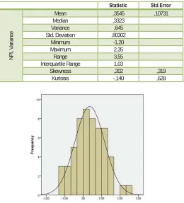
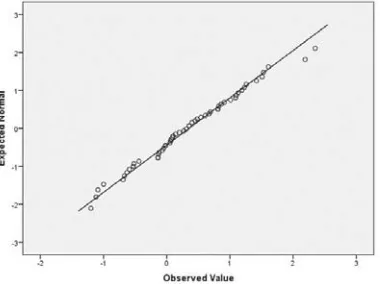
After we adjust the outliers and run again the descriptive statistics and normality test we achieve results shown on Table 1. From the Shapiro-Wilk test results we get a p-value=0.754 which is greater than our chosen alpha level. In this case we can't reject the null hypothesis that the data are normally distributed. To confirm this results we check the histogram (Figure 1) and Q-Q plot (Figure 2) of this distribution.
Table 1: Descriptive statistics (July 2001 - March 2016)
Statistic Std.Error
NPL Variance
Mean ,3545 ,10731
Median ,3323
Variance ,645
Std. Deviation ,80302
Minimum -1,20
Maximum 2,35
Range 3,55
Interquartile Range 1,03
Skewness ,202 ,319
Kurtosis -,140 ,628
Figure 2: Q-Q plot
From both the histogram and the Q-Q plot we confirm that the data distribution is adequately normal. After we confirmed the normal distribution of the data, now we can calculate the VaR for a confidence level of 95% and 99% (recommended for calculating risk exposure).
We repeat the same steps for the four time series for the respective quartiles, verify the normal distribution and calculate the respective VaR. The results are shown in the Table 2. To verify if our estimated values match the historical values, we calculate the historical VaR (Table 3) and compare the values with the statistical VaR.
Table 2: Statistical Value at Risk
Total 1stQ 2ndQ 3dQ 4th Q
Mean ,3545 ,6614 ,2546 ,3929 -,1482
St.Dev ,80302 ,6134 ,9078 ,8084 ,4909
VaR 99% 2,222623 2,088439 2,366554 2,273526 0,993929 VaR 95% 1,675372 1,670402 1,74787 1,722592 0,659352
Table 3: Historical Value at Risk
Total 1st Q 2nd Q 3d Q 4th Q
VaR 99% 2,2604 1,5568 2,0598 1,5272 0,8456
VaR 95% 1,546 1,344 1,539 1,516 0,588
If we compare the historical VaR with the estimated statistical VaR we can see that the historical values almost never exceed the statistical values (only in the initial model with 0.04% for the 99% level of confidence). That means that more than 99% of the historical data are below the estimated value of this model. The simple initial model would be:
ܰܲܮଽଽΨൌ ʹǤʹʹ͵ ܰܲܮ௧ିଵ
If we interpret the initial model we can state with a 99% level of confidence that NPL values for the next quarter will not increase more than 2.23%. This calculations can help in predicting the capital the bank needs to hold to cover the expected losses.
Returning to seasonality, if we compare the estimated values of the first model with the estimated values of the other models we can notice a significant difference between the values estimated for the 4th quarter and the other values.
that we make the prediction. Or create 2 models (if the difference of the other 3 is not significant), one for the 4th quarter
and one for the other quarters. If we consider seasonality we get the following model: ܰܲܮଽଽΨൌ ሺʹǤͲͺͻ כ ܳଵ ʹǤ͵ כ ܳଶ ʹǤʹͶ כ ܳଷ ͲǤͻͻͶ כ ܳସሻ ܰܲܮ௧ିଵ
In the model that takes seasonality into consideration we include four dummy variables (Q1-Q4) to specify the
period we want to forecast NPL variance with a 99% level of confidence. For example if we want to predict in March the future values for the 2nd quarter of the year than we replace Q2=1 and all the other dummy variables with 0.
5. Recommendations
• Based on the results of this study we strongly recommend that commercial banks in Albania need to start implement their own IRB models as complementary models to the standard method. Using VaR models or similar IRB models will only get better predictions over time by increasing the number of values on the time series.
• The Bank of Albania, as the supervisor authority, needs to start working to adjust the current legislation relying on the Basel Committee recommendations to permit the use of IRB models.
• From this study it is evident that seasonality is an important factor for predicting future NPL values. So banks can benefit from this information by taking less risk in the 2nd and 3d quarters and maximize the amount of business on the 4th quarter.
• We encourage other studies in other factors mentioned above like maturity period, borrower/loan quality etc. Studying these factors can help to improve and develop better predicting models.
References
Gregory, J. (2012). Counterparty Credit Risk and Credit Value Adjustment (2nd ed). United Kingdom:John Wiley & Sons Ltd. Canabarro, E. (2009). Counterparty Credit Risk. United Kingdom: PrintonDemand-Worldwide.
Bielecki T. R., Brigo D., Patras F. (2011). Credit Risk Frontiers. New Jersey: Wiley & Sons, Inc. Saunders A., Allen L. (2002). Credit Risk Measurement. New York: John Wiley & Sons, Inc. Benzschawel T. (2012). Credit Risk Modeling. United Kingdom: Incisive Media.
Hibbeln M. (2010). Risk Management in Credit Portfolios. Germany: Springer-Verlag.
Blundell A., Atkinson P. (2010). Thinking Beyond Basel III: Necessary Solutions for Capital and Liquidity. Journal: Financial Market Trends, Vol.2010/1
Giolli L. (2006) Un modello VAR per la misura del rischio di credito nelle banche. Italy: Universita di Bologna. Jorion P. (2007) Value at Risk (3d ed). New York: The McGraw-Hill Inc.