The June Phenomenon and the Changing Month of the Year Effect
Anthony Yanxiang Gu1
1 Professor of Finance, School of Business, State University of New York, Geneseo, USA
Correspondence: Anthony Yanxiang Gu, Professor of Finance, School of Business, State University of New York, Geneseo, USA. Tel: 1-585-245-5368. E-mail: [email protected]
Received: January 22, 2015 Accepted: April 3, 2015 Online Published: May 11, 2015 doi:10.5430/afr.v4n3p1 URL: http://dx.doi.org/10.5430/afr.v4n3p1
Abstract
Mean June return of the U.S. stock market is significantly negative since 2001 and the phenomenon is more apparent for large stocks. June return is negatively related to returns of all the other months and the coefficients are all statistically significant except for January and August, and June return is significantly negatively related to change in short interest. Meanwhile, April is the best month for the DJIA and S&P 500 and October is the best for the NASDAQ. The purpose of this study is to reveal the worst month of the U.S. stock markets in the new century and the dynamics of the month-of-the-year anomaly.
Keywords: Month-of-the-year-effect, June and September phenomena, Equity market
1. Introduction
Stock market anomalies have been one of the most intriguing issues in modern investments. The most puzzling empirical findings include the January effect – the abnormally large returns on common stocks in most months of January (Wachtel, 1942, and Rozeff and Kinney, 1976), and the weekend effect – the abnormally high average Friday returns and significantly negative average Monday returns (Cross, 1973, and French, 1980). Recently, Gu (2003, 2004) finds that the effects declined or disappeared after they became well known, specifically, the January effect is declining and disappearing since late 1980s, and the weekend effect was declining from late 1970s to late 1980s and even reversing, that is, mean return of Mondays are higher than that of Fridays since late 1980s. Hulbert (2008) and Ziemba (2010) show that the January effect is disappearing, He & He (2011) question whether the January effect is replaced by November effect. Easterday et al., (2009) report that the January effect does not occur in some years, while Ciccone (2011), Dzhabarov & Ziemba (2010), Mashruwala & Mashruwala (2011), Ziemba (2011) and Sikes (2014) argue that the January effect still appears in modern U.S. stock markets, particularly for small stocks. Mashruwala and Mashruwala (2011) show that stocks of high accruals quality (AQ) outperform low AQ stocks only in January.
There may be a month in the year when the stock market generally performs the worst. Browning (2003) and Baldwin (2003) believe that September is the month, Gu and Simon (2007) documented that mean September returns of the U.S. stock markets are significantly negative and are the lowest among the calendar months, and the phenomenon is more apparent for large stocks.
Here in this study we examine each month’s return of major U.S. stock indices from 2001 through 2013 and test whether September is still generally the worst month for the U.S. equity market as the market grows into the new century, and whether there is a month in the year when the U.S. stock market generally performs the best. The objective of the study is to reveal the worst month of the U.S. stock market in the new century and the dynamics of the month-of-the-year anomaly. The study proceeds as follows: Section 2 introduces the data, Section 3 reports the empirical findings, Section 4 explains the June return and related variables, and, Section 5 concludes.
2. The Data
3. Empirical Findings
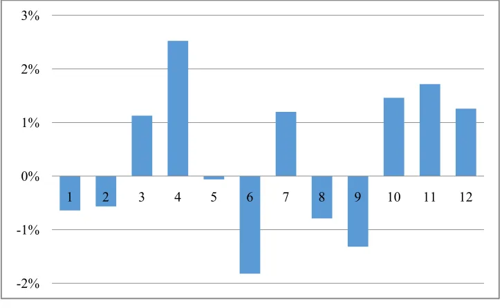
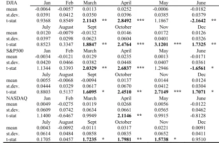
The mean monthly returns of the indices during the period are depicted in Figures 1 through 3 and the statistics of the empirical findings are presented in Table I. In the table, the mean and standard deviation of each month’s return for the three indices for the observation period is reported. The t-statistics in the column of June indicate the comparison of June return with 0 and the number below it is the statistical significance of the t-statistic for the observation period. The test is one-tailed, the null hypothesis is that June return is greater than or equal to zero, and the alternative hypothesis is that June return is less than zero. The t-statistics in the columns of the months other than June indicate the pairwise comparison of that month’s return with June return, and the number below it is the statistical significance of the t-statistic for the observation period. The test is one tailed, the null hypothesis is that June return is at least as much as that month’s return, and the alternative hypothesis is that June return is less than that month’s return.
Figure 1. DJIA Mean Monthly Return
Figure 2. S&P 500 Mean Monthly Return -2%
-1% 0% 1% 2% 3%
1 2 3 4 5 6 7 8 9 10 11 12
-2% -1% 0% 1% 2% 3%
Figure 3. NASDAQ Mean Monthly Return Table 1. Comparison of June Return with Return in Other Months
DJIA Jan Feb March April May June
mean -0.0064 -0.0057 0.0113 0.0252 -0.0006 -0.0182
st.dev. 0.0391 0.0412 0.0350 0.0396 0.0385 0.0379
t-stat 0.9368 0.8549 2.1143 ** 2.8492 *** 1.1867 -2.1642 **
July August Sept October Nov Dec
mean 0.0120 -0.0079 -0.0132 0.0146 0.0172 0.0126
st.dev. 0.0397 0.0298 0.0623 0.0604 0.0401 0.0326
t-stat 0.8523 0.3347 1.8847 ** 2.4764 *** 3.1201 *** 1.7325 **
S&P500 Jan Feb March April May June
mean -0.0034 -0.0121 0.0129 0.0235 0.0013 -0.0171
st.dev. 0.0420 0.0466 0.0382 0.0448 0.0407 0.0361
t-stat 1.1344 0.3393 2.0329 ** 2.6837 *** 1.2946 -1.6561 *
July August Sept October Nov Dec
mean 0.0055 -0.0068 -0.0094 0.0137 0.0144 0.0124
st.dev. 0.0444 0.0329 0.0617 0.0670 0.0412 0.0304
t-stat 0.8803 0.5137 1.6095 * 2.4510 ** 2.7149 *** 1.7071 *
NASDAQ Jan Feb March April May June
mean 0.0049 -0.0275 0.0119 0.0268 0.0056 -0.0122
st.dev. 0.0609 0.0742 0.0634 0.0661 0.0565 0.0462
t-stat 1.1400 -0.6467 0.9949 2.1146 ** 0.9915 -0.8128
July August Sept October Nov Dec
mean 0.0043 -0.0092 -0.0111 0.0317 0.0221 0.0091
st.dev. 0.0614 0.0484 0.0858 0.0835 0.0652 0.0411
t-stat 0.1705 0.0457 1.7235 * 1.7981 ** 1.5738 * 0.9510
1. t-statistics for the hypothesis that June mean is less than the given month’s mean 2. t-statistics for the hypothesis that June mean is less than zero
* Significance at the 10% level ** Significance at the 5% level *** Significance at the 1% level
The data covers 2001-2013. In addition to the mean return and standard deviation of the months, the column for each month other than June shows the t-statistic1 of pairwise comparison of that month’s return with June return, and the significance level. The column for June shows the t-statistic2 of comparing June return with zero, and the significance level.
-3% -2% -1% 0% 1% 2% 3% 4%
As shown in Table I, mean June return is significantly negative for all the three indices for the observation period. Specifically, for the DJIA Index, the mean is -1.82 percent (t-statistic = -2.16); for the S&P 500 Index, the mean is -1.71 percent (t-statistic = -1.66), and for the NASDAQ Composite Index, the mean is -1.22 percent (t-statistic = -0.81). The mean June return is even significantly lower than the mean September return, and mean September return is the second lowest for the DJIA, the third lowest for the S&P 500 and the NASDAQ. This indicates that the September phenomenon is declining in the last ten years after it became well known. Further observation is required to find whether the June anomaly will also diminish as it becomes well known in the future.
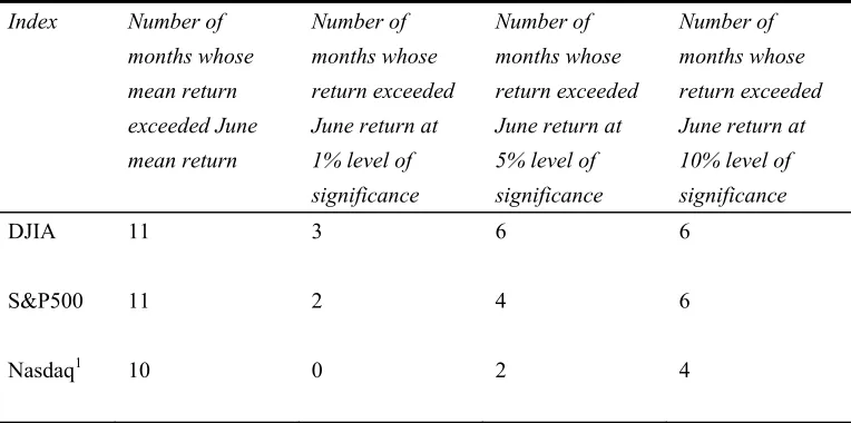
Mean June return is the lowest compared to all the other months for the DJIA and the S&P 500 indices from 2001 to 2013, and for the NASDAQ from 2002 to 2013, because February return of the NASDAQ Composite Index is negative 22.4 percent in 2001 as a result of the burst of the dot-com bubble, which made the mean of February returns of the tech-heavy index the lowest when year 2001 is included. Nonetheless, the difference between mean returns of February and June is not statistically significant for the NASDAQ index for the whole observation period. Table 2. Comparative Performance of June Return with Return in Other Months
Index Number of
months whose mean return exceeded June mean return
Number of months whose return exceeded June return at 1% level of significance
Number of months whose return exceeded June return at 5% level of significance
Number of months whose return exceeded June return at 10% level of significance
DJIA 11 3 6 6
S&P500 11 2 4 6
Nasdaq1 10 0 2 4
1. 11 if February 2001 return is excluded.
The data for this table is taken from Table I. Column 2 is the number of the 11 months whose mean return exceeded June mean return in the given time period, Columns 3, 4, and 5, are the number of months whose return exceeded June return at 1, 5, and 10 percent levels respectively.
The comparison results are summarized in Table II. In this table, column 2 shows the number of the other 11 months whose mean return exceeded mean June return, and column 3 shows the number of months whose mean return exceeded mean June return at the 1 percent level of significance. For example, for the DJIA Index during the period, there were three months (April, October, and November) whose mean return exceeded mean June return at the 1 percent level of significance. Column 4 shows the number of months whose return exceeded June return at the 5 percent level of significance. This includes those months where their mean returns exceeded mean June return at the 1 percent level of significance. Taking the DJIA Index as an example again, during the period, March, September and December mean return exceeded mean June return at the 5 percent level of significance, making a total of 6 months where their mean returns exceeded mean June return at the 5 percent level of significance. Column 5 shows the number of months whose mean return exceeded mean June return at the 10 percent level of significance. The number includes those months where their mean returns exceeded mean June return at the 1 percent and 5 percent levels of significance. For the DJIA Index, there were 6 months whose mean returns exceeded mean June return at the 10 percent level of significance.
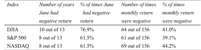
Table 3. Comparison of the Frequency of Negative Return in June with Negative Return in Other Months
Index Number of years
June had negative return
% of times June had negative return
Number of times monthly return were negative
% of times monthly return were negative
DJIA 10 out of 13 76.9% 64 out of 156 41.0%
S&P 500 8 out of 13 61.5% 61 out of 156 39.1%
NASDAQ 8 out of 13 61.5% 69 out of 156 44.2%
Column 2 shows the number of years June had a negative return for the given index and time period, column 3 expresses this as a percentage, column 4 gives the number of months where return was negative for the given index and number of months in the time period, and column 5 expresses that as a percentage.
In Table III, column 2 shows the number of years when June has a negative return, out of the total number of years in the sample period, and column 3 shows the percentage of years when June has negative return. For example, for the DJIA Index, 10 out of the 13 Junes in the period have negative returns, which is 76.9 percent. Column 4 shows the number of months in that time period which have negative returns, as well as the number of months included in that time period. For the DJIA Index, there were 64 months out of the 156 months when the return was negative. Column 5 shows this as a percentage, which in this case is 41 percent. It is clear that for every index, on a percentage basis, June return has significantly more often been negative compared to all of the other eleven months’ returns.
Mean June return is the lowest for large stocks because most of the June returns in the period are negative. However, June return in each year is not necessarily the lowest among the twelve months. This is different from the September phenomenon reported by Gu and Simon (2007) who point out that a significant percentage of September returns are the lowest in the year.
Mean June return of large stocks is more significantly negative than that of small stocks. The DJIA Index is composed of the thirty largest stocks; the S&P 500 Index contains the thirty largest stocks in the DJIA Index and other 470 smaller stocks; while the NASDAQ Composite Index contains a few thousand much smaller stocks. The percentage of Junes with negative return is much higher for the DJIA Index, which is 76.9 percent while for the NASDAQ Composite Index it is 61.5 percent. Small firm stocks perform better than large ones in the June phenomenon, or in other words, the negative performance is less pronounced for small firm stocks than large ones. This is similar to the September phenomenon and the January effect, i.e., small firm stocks were noticed to perform better than large ones in September (Gu and Simon, 2007), and even better than large firm stocks in January (Rozeff and Kinney, 1976, Reinganum, 1981, Keim, 1983, Roll, 1983, and Loughran, 1997).
We also examine which week(s) in June contribute(s) more to the month’s poor performance, similar to the examination by Wang, Li, and Erickson (1997) who found that Monday effect occurs primarily in the fourth and fifth weeks of the month. The first week of the month is defined as the week that contains the first trading Friday of the month. We find that the forth week is the worst followed by the first week for the DJIA and S&P 500 indices, and the difference between the two weeks’ returns and the second week’s returns are statistically significant at the 1 percent and 10 percent levels, respectively, for the DJIA, but insignificant for the S&P 500. Comparisons of other pairs of the weeks’ returns did not yield statistically significant results. For the NASDAQ, the third week appears the worst followed by the first week, but the differences between the two weeks’ returns and the second week’s returns are statistically insignificant.
April is the best month for large stocks, i.e., mean April returns are 2.5 percent and 2.4 percent for the DJIA and S&P 500, respectively. The absolute values of mean April returns are significantly larger than the absolute values of mean June returns for the three indexes. Further, frequency of positive April return is 10 and 9 for the DJIA and the S&P 500, respectively, the highest among the twelve months for the indexes in the sample period, even higher than the frequency of negative June returns for the S&P 500, which is 8.
the mean February and June returns of the NASDAQ, and also significantly larger than the mean June returns of the DJIA and the S&P 500 indexes.
4. June return and related variables
It is well talked about that a good January leads a good year of the stock market although we did not find any report of empirical evidence. To find possible relations between returns of June and the other eleven months, and the year, and changes in short interest, we conduct a regression analysis:
RJ = α + ∑βi Ri + δY + γS (1)
Where,
RJ = June return of each year
Ri = return of each of the other eleven months, i = 1, … 5, 7,…11
Yt = return of the year
S = change in short interest
Short interest reflects investors’ expectations and their actions. The NYSE releases monthly total short interest report every month, total short interest reflects investors’ expectations of the stock market’s movement and their actions may move the market. Change in short interest is calculated using the mid-month data, i.e., from min-May to mid-June, because of data availability (Note 1). Results of the regression analysis are presented in Table IV.
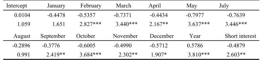
Table 4. Estimates from Regressing June Return on Related Variables
Intercept January February March April May July
0.0104 -0.4478 -0.5357 -0.7371 -0.4434 -0.7977 -0.7639
1.059 1.651 2.827*** 3.440*** 2.167** 3.637*** 3.446***
August September October November December Year Short interest
-0.2896 -0.3776 -0.6005 -0.4990 -0.5712 0.5786 -0.4879
0.991 2.419** 3.684*** 2.302** 1.907* 3.810*** 2.603**
* Significant at the 10% level. ** Significant at the 5% level. *** Significant at the 1% level.
The independent variables are returns of the other eleven months, the indices’ annual returns, and change in short interest. The adjusted R Square is 0.787.
As shown in Table IV, June return is negatively related to returns of all the other eleven months, and all the coefficients are statistically significant except for January and August. This indicates that generally, the more the indexes increase from January through May, the more they decline in June, and the more they decline in June, the more they increase from July to the end of the year. The relation between June return and return of the year is significantly positive, which indicates that a better (worse) June return may help (hurt) return of the year. The relation between June return and change in short interest is negative and statistically significant, this shows that generally, selling, including selling short dominates the market in the first half of June, which frequently results in negative June returns in the period.
Macroeconomic seasonality could also be a reason, but only thirteen years of macroeconomic data, i.e., GDP growth, inflation rate, unemployment rate, interest rate, housing market, consumer confidence, and change in international trade balance, does not result in meaningful statistics.
5. Conclusion
This study contributes to the literature the June phenomenon in the new century and related variables. Most of the Junes in the period have experienced negative returns for the DJIA, NASDAQ Composite and the S&P 500 indices, which appears that the September phenomenon is being replaced by June phenomenon. June return of the indices is negatively related to returns of all the other eleven months and all the coefficients are statistically significant except for January and August. June return is significantly positively related to return of the year. And June return is significantly negatively related to change in short interest. The implication of this finding is that one should sell late May, buy late June, as long as this phenomenon lasts. April returns are the highest for the DJIA and S&P 500, and October returns are the highest for the NASDAQ. Tax-loss selling and ‘window dressing’ could contribute to the poor June and good April performances. A market phenomenon should disappear after it is well known, and it is a puzzle why mean June return replaced mean September return as the lowest for the U.S. equity market in the last 10 years, and whether the June and April phenomena will continue and how long it will continue. Mid month to mid month returns, i.e., from the 16th of a month to the 15th of the next month may exhibit more significant monthly performance pattern. Further research is needed to answer these puzzles and questions.
Acknowledgements:
Thanks to the anonymous reviewers for their valuable comments and suggestions.
References
Baldwin, A. (2003). Historically, September is market’s worst month, Associated Press, New York, August 31. Browning, E. S. (2003). After hot summer for stocks, time to study, The Wall Street Journal, September 2, C1. Chang, E. C. & Pinegar, L. M. (1989), Seasonal fluctuations in industrial production and stock market seasonals,
Journal of Financial and Quantitative Analysis 24, 59-74. http://dx.doi.org/10.2307/2330748
, (1990). Stock market seasonal and prespecified multifactor pricing relations, Journal of Financial and Quantitative
Analysis 25, 517-33.
Ciccone, S.J. (2011). Investor optimism, false hopes and the January effect. Journal of Behavioral Finance, 12 , 158-168. http://dx.doi.org/10.1080/15427560.2011.602197
Cross F. (1973). The behavior of stock prices on Fridays and Mondays, Financial analysts Journal, 29, 67-69. http://dx.doi.org/10.2469/faj.v29.n6.67
Dzhabarov, C., & Ziemba, W.T. (2010). Do seasonal anomalies still work? Journal of Portfolio Management, 36, 93-104. http://dx.doi.org/10.3905/jpm.2010.36.3.093
Easterday, K. E., Sen, P. K., & Stephan, J. A. (2009). The persistence of the small firm/January effect: is it consistent with investors' learning and arbitrage efforts? Quarterly Review of Economics and Finance, 49, 1172-1193. http://dx.doi.org/10.1016/j.qref.2008.07.001
French, K. (1980). Stock Returns and the Weekend Effect, Journal of Financial Economics 8, 55-69. http://dx.doi.org/10.1016/0304-405X(80)90021-5
Gu, Anthony Y. (2003). The Declining January Effect: Evidence from U.S. Equity Markets. Quarterly Review of
Economics and Finance, 43(2): 395-404. http://dx.doi.org/10.1016/S1062-9769(02)00160-6
Gu, Anthony Y. (2004). The Reversing Weekend Effect: Evidences from U.S. Equity Markets, Review of
Quantitative Finance and Accounting, 22(1): 5-14.http://dx.doi.org/10.1023/B:REQU.0000006183.42549.50
Gu, Anthony Y. & Simon, J. (2007). The September Phenomenon of U.S. Equity Market, Advances in Quantitative
Analysis of Finance & Accounting, V5, 2007, 283-297. http://dx.doi.org/10.1142/9789812772213_0014
Haugen, R. A. & Lakonishok, J (1988). The Incredible January Effect: The Stock Market’s Unsolved Mystery (Dow Jones-Irwin, Homewood, IL).
Keim, D.B. (1983). Size related anomalies and stock return seasonality: Further empirical evidence, Journal of
Financial Economics 12, 13-32. http://dx.doi.org/10.1016/0304-405X(83)90025-9
Kohers, T. & Kohli, R. K. (1992). The yearend effect in stock returns over business cycles: a technical note, Journal
of Economics and Finance16, 61-68. http://dx.doi.org/10.1007/BF02919794
Kramer, C. (1994). Macroeconomic seasonality and the January effect, Journal of Finance, 49, 1883-91. http://dx.doi.org/10.2307/2329275
Ligon, J. (1997). A simultaneous test of competing theories regarding the January effect, Journal of Financial
Research 20, 13-32. http://dx.doi.org/10.1111/j.1475-6803.1997.tb00234.x
Loughran, T. (1997). Book-to-market across firm size, exchange, and seasonality: is there an effect? Journal of
Financial and Quantitative Analysis 32(3): 249-268. http://dx.doi.org/10.2307/2331199
Mashruwala, C.A., & Mashruwala, S.D. (2011). The pricing of accruals quality: January vs. the rest of the year. The
Accounting Review, 86, 1349-1381. http://dx.doi.org/10.2308/accr-10035
Reinganum, M. R. (1981). Misspecification of capital asset pricing: Empirical anomalies based on earnings’ yields and market values, Journal of Financial Economics 9, 19-46. http://dx.doi.org/10.1016/0304-405X(81)90019-2 Ritter, J.R. (1988). The buying and selling behavior of individual investors at the turn of the year, Journal of Finance
43, 701-17. http://dx.doi.org/10.1111/j.1540-6261.1988.tb04601.x
Ritter, J. R. & Chopra, N. (1989). Portfolio rebalancing and the turn-of the-year effect. Journal of Finance 44, 149-166. http://dx.doi.org/10.1111/j.1540-6261.1989.tb02409.x
Roll, R. (1983). On computing mean returns and the small firm premium, Journal of Financial Economics 12, 371-386. http://dx.doi.org/10.1016/0304-405X(83)90055-7
Rozeff, M. S. & Kinney W. R. Jr. (1976). Capital market seasonality: The case of stock returns, Journal of Financial
Economics 3, 379-402. http://dx.doi.org/10.1016/0304-405X(76)90028-3
Sikes, S.A. (2014). The turn-of-the-year effect and tax-loss-selling by institutional investors. Journal of Accounting
and Economics, 57, 22-42. http://dx.doi.org/10.1016/j.jacceco.2013.12.002
Wachtel, S. B. (1942). Certain observations on seasonal movements in stock prices, Journal of Business 15, 184-193. http://dx.doi.org/10.1086/232617
Wang, K., Li, Y. & Erickson, J. (1997). A New Look at the Monday Effect, Journal of Finance, 52(5) 2127-2186. http://dx.doi.org/10.1111/j.1540-6261.1997.tb02757.x
Ziemba, W.T. (2011). Investing in the turn-of-the-year effect. Financial Markets and Portfolio Management, 25, 455-472. http://dx.doi.org/10.1007/s11408-011-0170-1
Note