262 December, 2016 AgricEngInt: CIGR Journal Open access at http://www.cigrjournal.org Vol. 18, No. 4
Artificial neural network based modeling of tractor performance
at different field conditions
Salim Almaliki
1, Reza Alimardani
2*, Mahmoud Omid
2(1.Department of Agricultural Machinery, University of Basrah, Basrah, Iraq.
2.Department of Agricultural Machinery Engineering, College of Agriculture and Natural Resources, University of Tehran, Karaj, Iran)
Abstract: Application of tractors in farming is undeniable as a power supply. Therefore, performance model for evolving parameters of tractors and implements are essential for farm machinery, operators and manufacturers alike. The objective of this study was to assess the predictive capability of several configurations of ANNs for performance evaluating of tractor in parameters of drawbar power, fuel consumption, rolling resistance and tractive efficiency. A conventional tillage system which included a moldboard plow with three furrows was used for collecting data from MF285 Massey Ferguson tractor. To predict performance parameters, ANN models with back-propagation algorithm were developed using the MATLAB software with different topologies and training algorithms. For drawbar power, the best result was obtained by the ANN with 6-7-1 topology and Bayesian regulation training algorithm with R2 of 0.995 and MSE of 0.00024. The ANN model with 6-7-1 structure and Levenberg-Marquardt training algorithm had the best performance with R2 of 0.969 and MSE of 0.13427 for TFC prediction. The 6-8-1 topology shows the best power for prediction of AFC with R2 and MSE of 0.885 and 0.01348, respectively. Also, the 6-10-1 structure yielded the best performance for prediction of SFC with R2 of 0.935 and MSE of 0.012756. The obtained result showed that the 6-7-1 structured ANN with Levenberg-Marquardt training algorithm represents a good prediction of TE with R2 equal to 0.989 and MSE of 0.001327. The obtained results confirmed that the neural network can be able to learn the relationships between the input variables and performance parameters of tractor, very well.
Keywords: artificial neural network, tractive efficiency, rolling resistance, drawbar power, fuel consumption.
Citation: Almaliki, S., R. Alimardani, and M.Omid. 2016. Artificial neural network based modeling of tractor performance at different field conditions. Agricultural Engineering International: CIGR Journal, 18(4):262-274.
1 Introduction
1The great increase in agricultural productivity over
the last century can be related to mechanization,
particularly the development of the tractors. The main
function of tractors is to be interfaced with implements
that provide power, tractive effort to move the
implements through the field and control the implements.
It is necessary that we have the proper understanding of
how the tractor power can be used, and tractor-implement
systems can be optimized. The proper field machines'
operation is essential for any system to be reasonably
Received date: 2016-07-11 Accepted date: 2016-10-08 *Corresponding author: Reza Alimardani, Department of Agricultural Machinery Engineering, College of Agriculture and Natural Resources, University of Tehran, Karaj, Iran. Tel.: +989123332216. E-mail Address: [email protected]
profitable. Thus, efficient operation of farm tractors
includes: (a) maximizing fuel efficiency of the engine and
mechanical efficiency of the drive train, (b) maximizing
attractive advantage of traction devices and (c) selecting
an optimum travel speed for a given tractor‐implement
system (Grisso et al., 2008). Therefore, performance
model for evolving parameters of tractors and implements
are essential for farm machinery operators and
manufacturers alike.
The modeling techniques used in mechanization
processes are quite important to provide an accurate and
sustainable use of power resources. One of the most
popular techniques for modelling and forecasting
behavior of nonlinear systems is soft computing. Soft
computing technology is an interdisciplinary research
December, 2016 Artificial neural network based modeling of tractor performance at different field conditions Vol. 18, No. 4 263
techniques are being used in soft computing such as
statistics, machine learning, neural network and fuzzy
logic for exploratory data analysis (Carman, 2008). In
recent years, the methods of artificial intelligence (AI)
have widely been used in different areas including
agricultural applications (Safa et al., 2009; Douik and
Abdellaoui, 2008; Kashaninejad et al., 2009). The
application of soft computing to AI is studied collectively
by the emerging discipline of computational intelligence
(CI) for example, artificial neural networks (ANN). These
methods are inspired by the central nervous system,
exploiting features such as high connectivity and parallel
information processing, exactly like in the human brain
(Arriagada et al., 2002). Several researchers focused on
artificial intelligence for modeling of different component of agricultural systems (Cakmak and Yıldız, 2011;
Zarifneshat et al., 2012; Çay et al., 2013; Aghbashlo et al.,
2012; Khoshnevisan et al., 2013; Young et al., 2013; Safa
and Samarasinghe, 2013). For example Aghbashlo et al.
(2012) developed a supervised ANN and mathematical
models for determining the exegetics performance of a
spray drying process. They were concluded that the MLP
(multilayer perceptron) ANN approach for exegetics
prediction of spray drying process was capable of
yielding good results and that could be considered as an
attractive alternative to traditional regression models and
other related statistical approaches. Cakmak and Yıldız
(2011) used ANN to determine the drying rate of seedy
grapes. Input parameters used for the ANN model were
the moisture content, the hot air temperature and the hot
airflow rate. The structure of the ANN model with one
hidden layer was determined considering different neuron
numbers at the hidden layer. Based on error analysis
results, they concluded Levenberge Marquardt
optimization technique was the most appropriate method
for prediction capability of transient drying rates.
Zarifneshat et al. (2012) applied ANN to predict apple's
bruise volume. The network was trained using two
learning algorithms: BB (Basic Backpropagation) and
BDLRF (Backpropagation with Declining Learning Rate
Factor). They reported that BDLRF algorithm yields a
better performance than BB algorithm. Developments of
prediction equations for tire tractive performance have
been the focus of much research. Artificial Neural
Networks (ANNs) have been accepted as a potentially
useful tool for modeling complex non-linear systems and
widely used for prediction (Nayak et al., 2004). Many
researchers have reported the proper ability of ANN
versus regression method such as study done by Rahimi
and Abbaspour (2011). They used artificial neural
network and stepwise multiple range regression methods
for prediction of tractor fuel consumption. Their results
showed that ANN provided better prediction accuracy
compared to stepwise regression. Roul et al. (2009)
successfully applied ANN representation predicting the
draught requirement of tillage implements under varying
operating and soil conditions.
A neural network is adjusted for a definite task such
as model distinguishing and data classification during a
training process. Extensive aptitude of this approach for
accurate estimations of complicated regressions
contributes more advantage compared to classical
statistical techniques. Bietresato et al. (2015) assessed the
predictive capability of several configurations of ANNs
for evaluating indirectly performance (torque, BSFC) of
diesel engines employed in agricultural tractors. The
results showed the ANNs with the outlined characteristics
proved to be useful and reliable tools for correlating EG
temperature and rpms with torque and BSFC. Ekinci et al.
(2015) used ANNs and two types of Support Vector
Regression (SVR) models to predict the tractive
efficiency. The results showed that the ANN model
trained using Levenberge Marquardt algorithm has
produced more accurate results.
The objective of this study was to assess the
predictive capability of several configurations of ANNs
for performance evaluating of tractor in parameters of
drawbar power, fuel consumption, rolling resistance and
264 December, 2016 AgricEngInt: CIGR Journal Open access at http://www.cigrjournal.org Vol. 18, No.4
2 Materials and methods
2.1 Field experiments
In this research, a conventional tillage system
which includes a moldboard plow with three furrows
(width of mold board was 100 cm) was used for
collecting data from Massey Ferguson tractor (Model
MF285). The specifications of tractor showed in Table 1.
The experiments were carried out in the field with
different conditions using three engine speeds, four
tractor forward speeds (as shown in Table 2), three depths
of moldboard plow and three tire Inflation pressures,
These parameters were used at two moisture contents and
four cone indexes of soils as shown in Table 2. Table 3
shows the actual velocity of the tractor at different engine
speed and gears.
Table 1 Specifications of Massey Ferguson MF285
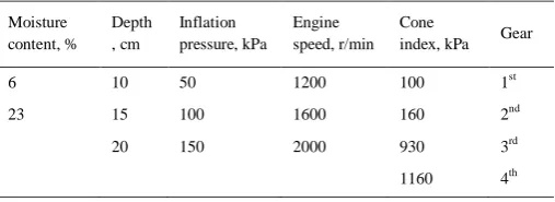
Table 2 Input parameters used in experiments
Moisture content, % Depth , cm Inflation pressure, kPa Engine speed, r/min Cone
index, kPa Gear
6 10 50 1200 100 1st
23 15 100 1600 160 2nd
20 150 2000 930 3rd
1160 4th
Table 3 Velocities used in experiments (m/s)
Engine speed, r/min Gear
1st 2nd 3rd 4th
1200 0.39 0.56 0.79 1.09
1600 0.48 0.67 0.95 1.28
2000 0.61 0.90 1.2 1.56
2.2 Calculation of parameters
2.2.1 Drawbar power
Drawbar power is obtained using the relation
between draft and travel speed as Equation 1:
a db
NT
V
P
(1)where Pdb is drawbar power (kW), NT is net traction (kN)
and Va is actual velocity (m/s).
2.2.2 Fuel consumption
The fuel amount required for each tillage operation
was determined by two flow sensors: one for measuring
input fuel to injector pump and another on returning fuel
line to the tank.
In this research, the expressions of characteristics of
fuel consumption of engine farm tractor are in three terms
as; Temporal Fuel Consumption (TFC), Area-specific
Fuel Consumption (AFC) and Specific Fuel Consumption
(SFC).
TFC represents the amount of fuelconsumed for the unit
of time according to the following Equation 2:
T
fc
TFC
(2)
Where fc is fuel consumption at taken time (L/h) and T is
time taken (h).
AFC represents the amount of fuelconsumed to cover an
area of one hectare and is calculated according to the
following Equation 3:
W
V
TFC
AFC
a
10
(3)Where TFC is fuel consumption (L/h), W is implement
working width (m) and Va is actual velocity of the tractor
(m/s).
Item Parameters
Effective output, hp Type of fuel
75 Diesel
Type of steering system Mechanical- hydraulic
Transmission Gears
Type of injector pump Rotary
Firing order 1342
Fuel tank capacity, L 90
Lifting capacity, kg 2227
Rated engine speed, r/min 2000
Type of cooling system Liquid-cooled
Front tires size, inch 12.4-24
Rear tires size, inch 18.4-30
Front Weight, kg 1420
Rear Weight, kg 1694
Total Weight, kg 3114
December, 2016 Artificial neural network based modeling of tractor performance at different field conditions Vol. 18, No. 4 265
SFC represents the amount of fuelconsumed during a
specified time on the basis of the drawbar poweravailable
at the drawbar, it is calculated as Equation 4:
db
P
TFC
SFC
(4)2.2.3 Rolling resistance
Rolling resistance of the tractor was measured by a
dummy tractor towing the test tractor through load cell
connected to a digital load indicator. Rear tractor was kept
in neutral position while the front tractor pulled the rear
one. The reading of load indicator was noted from digital
indicator at determined time interval. An average of four
readings was considered in computing the force required
to pull a tractor.
The drawbar load cell was an S shape (model:
H3-C3-3.0 t-6B-D55 from Zemic with capacity of 30 kN)
mounted between two tractors.The first one was a Massey
Ferguson 285 as puller and the other one was Massey
Ferguson 165 as auxiliary. The auxiliary tractor pulls the
implement-mounted tractor with the latter in neutral gear
but with the implement in the operating position. The force
exerted by the implement is measured by a strain gauge
Wheatstone bridge arrangement.Draft was recorded in the
measured distance (20 m) as well as the time taken to
traverse the distance. Calibrations of the load cell were
conducted against known loads by a hydraulic loading
device from INSTRON (Model 4486).
2.2.4 Tractive efficiency
Tractive efficiency (TE) is defined as; ability of tractor
to transfer power from the axle input to the soil through
wheels. TE depends on slip (set by ballast), soil conditions,
tires and drive configurations and is calculated using
Equation 5: 100 ) ( 100 ) ( power axele power drawbar power input power output
TE (5)
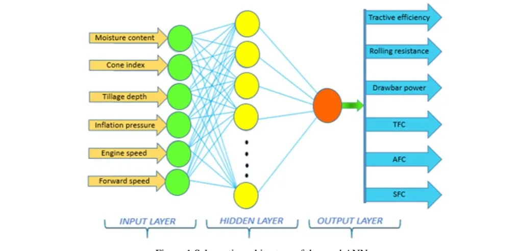
2.3 ANN model design
In this study, to predict performance parameters,
ANN models with back-propagation algorithm were
developed using MATLAB software (Demuth and Beale,
1998). Generally, the ANN is characterized by three
layers: an input layer, a hidden layer, and an output layer.
The acquired data was usually divided into three
randomly selected subsets which include: 70% of the
dataset for training, 15% for model validation and 15%
for testing. Seven different training algorithms of gradient
descent with momentum (traingdm), Gradient descent
with momentum and adaptive learning rate (traingdx),
Bayesian regulation (trainbr), scaled conjugated gradient
(trainscg), Resilient (trainrp), Gradient descent with
adaptive learning rate (traingda) and
Levenberg-Marquardt (trainlm) were used for network
training. In general, there is not a specific method for
defining number of hidden layers and also number of
neurons in the hidden layer; so the number of neurons in
the hidden layer was obtained by trial and error method.
In this research, the number of hidden layers and neurons
in the hidden layer (or layers) were chosen by comparing
performance of the designed networks. Also, the
functions of tangent hyperbolic conversion, sigmoid and
linear motion function among layers were used. The
ANN system applied for these prediction models had six
inputs and a single output. The input vector included
depth, forward speed, engine speed, inflation tire,
moisture content and cone index of soil and the output of
the ANNs were drawbar power, TFC, AFC, SFC, rolling
resistance and TE. The schematic architecture of the used
266 December, 2016 AgricEngInt: CIGR Journal Open access at http://www.cigrjournal.org Vol. 18, No.4
The input model consists of dendritic nodes similar
to a biological cell that could be represented as a vector
with N items X= (X1, X2,… , Xn); the summation of
inputs multiplied by their corresponding weights could be
represented by scalar quantity S. See Equation 6.
∑ (6)
where W=(W1 ,W2 ,… ,WN) is the weight vector of
associations among neurons. The S quantity is then
inserted into a non-linear conversion function f, yielding
the following output as Equation 7:
(7)
Non-linear transfer function is usually represented as
sigmoid functions and is defined via Equation 8:
(8)
The output of y can be as a result of the model or
that of the next layer (in multilayer networks). In the
design of an ANN, certain elements should be taken into
account including type of input parameters.
Prior to the utilization of dataset for model
development, the inputs and target output were normalized
or scaled linearly between -1 and 1 in order to increase the
accuracy, performance and speed of ANN.
To evaluate performance of developed models,
various criteria were used to calculate errors. Mean
square error (MSE) criterion which is a well-known
standard error is often used as a criterion to compare error
aspects in various models. Coefficient of determination
(R2) which is a method to calculate a standard error in
estimating methods shows the normal difference of real
data from the estimated data. The expressions for these
statistical measures are given as Equation 9 and Equation
10:
Ni
x
ix
iN
MSE
1
1(
ˆ
)
2 (9)2 1 1 2 1 2 2
)
(
)
ˆ
ˆ
(
[
)]
)(
ˆ
ˆ
(
[
Ni i iN i
N
i i i
x
x
x
x
x
x
x
x
R
(10)where N is the number of test observation, shows the
value of the variable being modeled (observed data), ̂
shows the value of variable modeled (predicted), and ̅
is the mean value of the variable.
3 Results and discussion
In this research, a computer program has been
developed under MATLAB software environment for
designing of ANNs based models for prediction of tractor
performance’s parameters. To evaluate the best fitting
model, MSE and R2 as index of network performance,
were utilized.
December, 2016 Artificial neural network based modeling of tractor performance at different field conditions Vol. 18, No. 4 267 3.1 Drawbar power
Table 4 shows result of ANN modeling using
different training algorithms. As a whole, all training
algorithm represented acceptable results. The best result
was obtained by the ANN with 6-7-1 topology and
Bayesian regulation training algorithm with R2 of 0.995
and MSE of 0.00024. Figure 2 shows regression result of
6-7-1 ANN model in training, validation and test mode.
The closeness between the predicted and actual values
promoted the accuracy of the network in prognostication
of the drawbar power. The results are in agreement with
the result of ElWahed and Aboukarima (2007). They
developed ANN model to predict drawbar pull of chisel
plow using forward speed, plowing depth, nominal tractor
power, rated plow width, soil texture index, initial soil
moisture content and initial soil specific weight as
independent variables. They reported the R2 value of the
developed model was more than 0.93.
Table 4 Optimum structure ANN models developed
by different training algorithms
Training algorithm
Optimum
topology Epochs MSE R2
Trainbr 6-7-1 35 0.000245 0.995
Trainlm 6-6-1 49 0.000257 0.996
Trainrp 6-7-1 96 0.001153 0.988
Trainscg 6-9-1 78 0.001200 0.913
Traingda 6-1-1 100 0.002485 0.979
Traingdx 6-1-1 100 0.004366 0.955
Traingdm 6-6-1 100 0.033402 0.848
268 September, 2016 AgricEngInt: CIGR Journal Open access at http://www.cigrjournal.org Vol. 18, No. 3 3.2 Fuel consumption
Three parameters of TFC, AFC and SFC were
modeled using ANNs. Table 5 represents different
structures of ANNs. Results show that the ANN model
with 6-7-1 structure and Levenberg-Marquardt training
algorithm had the best performance with R2 of 0.969 and
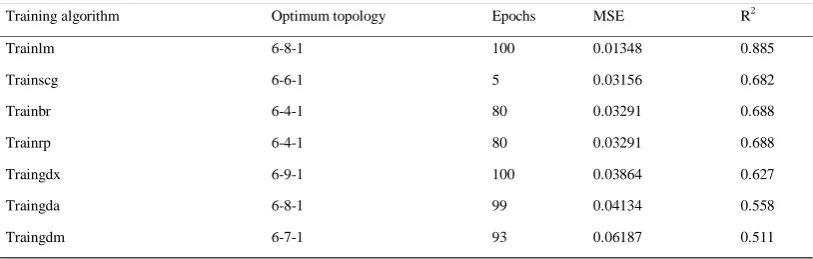
MSE of 0.13427 for TFC prediction. Also for AFC and
SFC, the Levenberg-Marquardt training algorithm yielded
the best results (Table 6 and Table 7). The 6-8-1 topology
shows the best power for prediction of AFC with R2 and
MSE of 0.885 and 0.01348, respectively. Also, the 6-10-1
structure yielded the best performance for prediction of
SFC with R2 of 0.935 and MSE of 0.012756. Gradient
descent with momentum and adaptive learning rate
(traingdx), gradient descent with momentum (traingdm),
Gradient descent with momentum and adaptive learning
rate (traingdx) and Bayesian regulation (trainbr) were
not responded in predicting for TFC while Gradient
descent with momentum and adaptive learning rate
(traingdx), gradient descent with momentum (traingdm),
Gradient descent with momentum and adaptive learning
rate (traingdx) and Resilient (trainrp) were not responded
in predicting for SFC. During training process some
training algorithms caused the error not to decrease, so
the process was diverging. As a result the algorithm
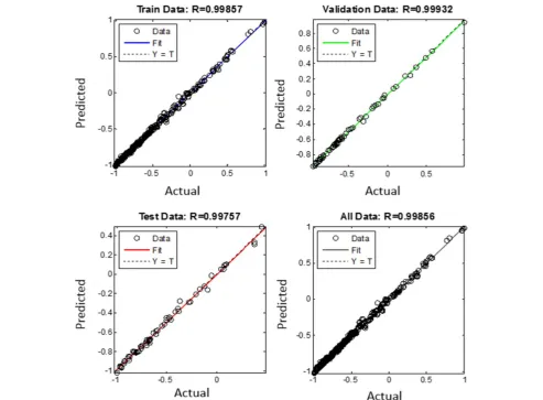
marked as not responding method. The regression graphs
represent the relationship between actual and predicted
values of the ANN, in the training, validation and test sets
that are illustrated in Figure 3, Figure 4 and Figure 5 for
TFC, AFC and SFC, respectively. The closeness of the
scattered data to the unity slope line is the representative
of the satisfactory performance of the optimal model.
Rahimi-Ajdadi and Abbaspour-Gilandeh (2011) obtained
the same result in fuel consumption prediction of tractor.
They assumed that fuel consumption to be a function of
engine speed, throttle and load conditions, chassis type,
total tested weight, drawbar and PTO power. They
adopted Back propagation Artificial Neural Network
(ANN) models with different training algorithms and
reported that the highest performance was obtained for
the network with two hidden layers each having 10
neurons which employed Levenberg–Marquardt training
algorithm with R2 of 0.986.
Table 5 Different networks structure to predict TFC
Training algorithm Optimum topology Epochs MSE R2
Trainlm 6-7-1 100 0.013427 0.969
Trainrp 6-8-1 76 0.042401 0.735
Trainscg 6-10-1 100 0.048406 0.604
Trainbr Not responding - - -
Traingdx Not responding - - -
Traingda Not responding - - -
Traingdm Not responding - - -
Table 6 Optimum models for AFC prediction
Training algorithm Optimum topology Epochs MSE R2
Trainlm 6-8-1 100 0.01348 0.885
Trainscg 6-6-1 5 0.03156 0.682
Trainbr 6-4-1 80 0.03291 0.688
Trainrp 6-4-1 80 0.03291 0.688
Traingdx 6-9-1 100 0.03864 0.627
Traingda 6-8-1 99 0.04134 0.558
269 September, 2016 AgricEngInt: CIGR Journal Open access at http://www.cigrjournal.org Vol. 18, No. 3
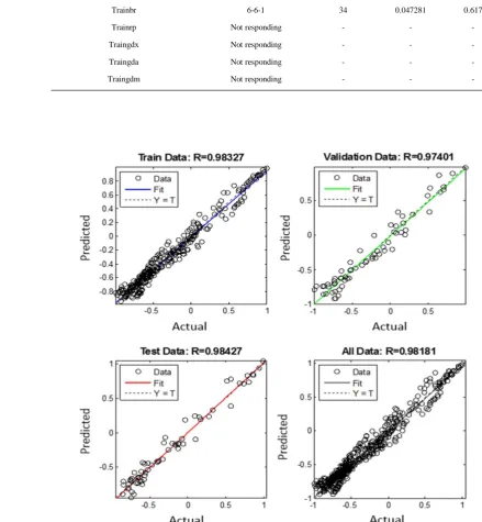
Table 7 Optimum models for SFC prediction
Training algorithm Optimum topology Epochs MSE R2
Trainlm 6-10-1 54 0.012756 0.935
Trainscg 6-6-1 65 0.043969 0.650
Trainbr 6-6-1 34 0.047281 0.617
Trainrp Not responding - - -
Traingdx Not responding - - -
Traingda Not responding - - -
Traingdm Not responding - - -
270 December, 2016 AgricEngInt: CIGR Journal Open access at http://www.cigrjournal.org Vol. 18, No.4
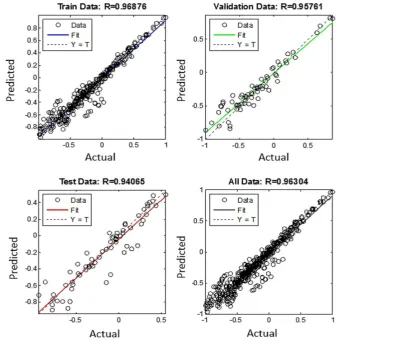
Figure 4 Regression result of the best ANN for AFC by Levenberg-Marquardt training algorithm
December, 2016 Artificial neural network based modeling of tractor performance at different field conditions Vol. 18, No. 4 271 3.3 Rolling resistance
As shown in Table 8, among adopted models, the
ANNs with Bayesian regulation and
Levenberg-Marquardt training algorithms had the best
results. But Levenberg-Marquardt algorithm yield the
least error (MSE= 0.000783) and reached to the minimum
error at epoch 88, faster than Bayesian regulation (Epoch
96). Figure 6 illustrates the result of 6-10-1 structured
analysis. The inconsiderable difference between the
predicted and actual values corroborated the reliability of
the network in predicting the rolling resistance.
Taghavifar et al. (2013) reported the same results. They
adopted a 3-10-1 feed-forward Artificial Neural Network
(ANN) with back propagation (BP) learning algorithm to
estimate the rolling resistance of wheel as affected by
velocity, tire inflation pressure, and normal load acting on
wheel inside the soil bin facility creating controlled
condition for test run. The model represented MSE of
0.0257 and predicted relative error values with less than
10% and high R2 equal to 0.9322 utilizing experimental
output data obtained from single-wheel tester of soil bin
facility.
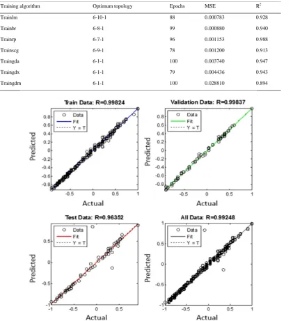
Table 8 Different ANN structures for rolling resistance prediction
Training algorithm Optimum topology Epochs MSE R2
Trainlm 6-10-1 88 0.000783 0.928
Trainbr 6-8-1 99 0.000880 0.940
Trainrp 6-7-1 96 0.001153 0.988
Trainscg 6-9-1 78 0.001200 0.913
Traingda 6-1-1 100 0.003740 0.947
Traingdx 6-1-1 79 0.004436 0.943
Traingdm 6-1-1 100 0.028810 0.894
Figure 6 Result of regression analysis for rolling resistance predictor based 6-10-1 structure and Levenberg-Marquardt
272 September, 2016 AgricEngInt: CIGR Journal Open access at http://www.cigrjournal.org Vol. 18, No. 3 3.4 Tractive efficiency (TE)
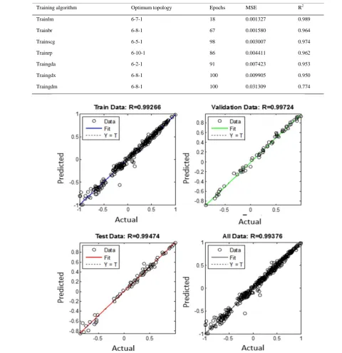
To predict TE parameter of the tractor, ANNs with
different topology and training algorithms were adapted.
The obtained result showed that the 6-7-1 structured
ANN with Levenberg-Marquardt training algorithm
represents a good prediction of TE with R2 equal to 0.989
and MSE of 0.001327 (Table 9). Figure 7 presents result
of regression analysis for TE. The small variation
between the predicted and measured values confirmed the
reliability of the network in predicting the tractive
efficiency. The similar result was reported by Taghavifar
and Mardani (2014). They used neuro-fuzzy inference
system (ANFIS) for TE prediction of agricultural tractor
driving wheel. The input parameters were wheel load,
velocity and slippage. They obtained MSE equal to
1.5676 and R2 equal to 0.97 for TE. Çarman and Taner
(2012) developed an ANN model with a back propagation
learning algorithm to predict TE of a driver wheel in clay
loam soil. They obtained mean relative error and R2 equal
to 1.33% and 0.999, respectively.
Table 9 Different ANN structures for TE
Training algorithm Optimum topology Epochs MSE R2
Trainlm 6-7-1 18 0.001327 0.989
Trainbr 6-8-1 67 0.001580 0.964
Trainscg 6-5-1 98 0.003007 0.974
Trainrp 6-10-1 86 0.004411 0.962
Traingda 6-2-1 91 0.007423 0.953
Traingdx 6-8-1 100 0.009905 0.950
Traingdm 6-8-1 100 0.031309 0.774
December, 2016 Artificial neural network based modeling of tractor performance at different field conditions Vol. 18, No. 4 273
4 Conclusion
This research represents ANN models for predicting
tractor performance parameters. Back propagation neural
networks with different training algorithms were
examined. On the basis of statistical performance criteria
of MSE and R2, it was found that for drawbar power the
ANN with Bayesian regulation training algorithm showed
the best prediction power and for TFC, AFC SFC rolling
resistance and TE, the ANNs with Levenberg–Marquardt
training algorithm represented the best results. The
obtained results confirmed that the neural network can be
able to learn the relationships between the input variables
and performance parameters of tractor, very well.
Eventually, it can be claim that the ANN models can be
suggested to predict performance of tractor because of
fast, accurate and reliable results, effectively.
Acknowledgement
The authors wish to thank all of the Iraqi Ministry of
Education, Basrah University and Department of
Agricultural Machinery Engineering, College of
Agriculture and Natural Resources, University of Tehran,
Karaj, Iran for providing necessary funds and research
facilities required for this investigation.
References
ElWahed, A. and M. Aboukarima. 2007. Draft models of chisel plow based on simulation using artificial neural networks. Misr Journal of Agricultural Engineering,
24(1):42-61.
Aghbashlo, M., H. Mobli, S. Rafiee, and A. Madadlou. 2012 The use of artificial neural network to predict exegetic performance of a spray drying process: a preliminary study. Computers & Electronics in Agriculture, 88(2):32-43.
Arriagada, J., P. Olausson, and A. Selimovic. 2002 Artificial neural network simulator for SOFC performance prediction.
Journal of Power Sources, 112(1):54-60.
Bietresato, M., A. Calcante, and, F. Mazzetto. 2015. A neural network approach for indirectly estimating farm tractors engine performances. Fuel, 143(2015):144-154.
Cakmak, G., and C. Yıldız. 2011. The prediction of seedy grape drying rate using a neural network method. Computers & Electronics in Agriculture, 75(1):132-138.
Carman, K. 2008. Prediction of soil compaction under pneumatic tires a using fuzzy logic approach. Journal of Terramechanics, 45(4):103-108.
Çarman, K., and A. Taner. 2012. Prediction of tire tractive performance by using artificial neural networks. Mathematical and Computational Applications, 17(3):182-192.
Çay, Y., I, Korkmaz, A, Çiçek, and F. Kara. 2013. Prediction of engine performance and exhaust emissions for gasoline and methanol using artificial neural network. Energy, 50(1):177-186.
Demuth, H., and M. Beale. 1998. Neural Network Toolbox for Use with Matlab the Mathworks Inc. January 1998.
Douik, A., and M. Abdellaoui. 2008. Cereal varieties classification using wavelet techniques combined to multi-layer neural networks. 16th Mediterranean Conference on Control and Automation, France, 1822-1827
Ekinci, S., K. Çarman, and H. Kahramanlı. 2015. Investigation and modeling of the tractive performance of radial tires Using off-road vehicles. Energy, 93:1953-1963.
Grisso, R. D., D. H. Vaughan, and G. T. Roberson. 2008. Fuel prediction for specific tractor models. Applied Eng. Agric.,
24(2008):423-428.
Kashaninejad, M., A. A. Dehghani, and M. Kashiri. 2009. Modeling of wheat soaking using two artificial neural networks (MLP and RBF) Journal of Food Engineering,
91(4):602-607.
Khoshnevisan, B., S. Rafiee, M. Omid, M. Yousefi, and M. Movahedi. 2013. Modeling of energy consumption and GHG (greenhouse gas) emissions in wheat production in Esfahan province of Iran using artificial neural networks. Energy,
52(1):333-338.
Nayak, P. C., K. P. Sudheer, D. M. Ragan, and K. S. Ramasastri, 2004. A neuro fuzzy computing technique for modeling hydrological time series. Journal of Hydrology, 29(1-2):52-66. Rahimi, A. F., and G. Y. Abbaspour. 2011. Artificial neural network and stepwise multiple range regression methods for prediction of tractor fuel consumption. Measurement,
44(10):2104-2111.
Roul, A. K., H. Raheman, M. S. Pansare, and R. Machavaram. 2009. Predicting the draught requirement of tillage implements in sandy clay loam soil using an artificial neural network. Biosystems Engineering, 104(4):476-485.
Safa, M., S. Samarasinghe, and M. Mohsen, 2009. Modeling fuel consumption in wheat production using neural networks. In: Proceedings of the 18th world IMACS/MODSIM Congress, Australia; July 2009. Pp. 775-781
274 December, 2016 AgricEngInt: CIGR Journal Open access at http://www.cigrjournal.org Vol. 18, No.4 Taghavifar, H., and A. Mardani. 2014. On the modeling of energy
efficiency indices of agricultural tractor driving wheels applying adaptive neuro-fuzzy inference system. Journal of Terramechanics, 56:37-47.
Taghavifar, H., A. Mardani, H. Karim-Maslak, andH. Kalbkhani. 2013. Artificial Neural Network estimation of wheel rolling resistance in clay loam soil. Applied Soft Computing, 13(8):3544-3551.
Young, J. S., Y. P. Lin, and P. W. Shih. 2013. Neural network approach to gain scheduling for traction control of electrical vehicles. Applied Mechanics and Materials, 392:272-276. Zarifneshat, S., A. Rohani, H. R. Ghassemzadeh, M. Sadeghi, E.