A Novel Wireless Sensor Network Evolution Model
Based on Energy-Efficiency
https://doi.org/10.3991/ijoe.v13i03.6855
Hui Gao*
Zhengzhou Railway Vocational & Technical College, Zhengzhou City, China [email protected]
Zhixian Yang
Zhengzhou Railway Vocational & Technical College, Zhengzhou City, China [email protected]
Abstract—The Barabási–Albert (BA) model is a famous complex network model that generates scale-free networks. Wireless sensor networks (WSNs) had been thought to be approximately scale-free through lots of empirical re-search. Based on the BA model, we propose an evolution model for WSNs. Ac-cording to actual influence factors such as the remainder energy of each sensor and physical link capability of each sensor, our evolution model constructs WSNs by using a preferential attachment mechanism. Through simulation and analysis, we can prove that our evolution model would make the total energy consumption of the WSNs more efficient and have a superior random node er-ror tolerance.
Keywords—Wireless sensor network; Complex networks; Evolution model; Energy-aware; Energy-balanced
1
Introduction
WSNs, which are usually called wireless sensor and actuator networks (WSANs) [1], are remotely located wireless sensors to monitor realistic conditions, and to bi-directionally transfer information by the networks to a master position. The improve-ment of WSNs originated in some special applications such as natural disaster relief. Now WSNs are used widely in many societal fields, such as industry supervisory control, machinery equipment performance monitoring, traffic control, and so on [2, 3].
the limited energy to effectively balance the energy consumption of each sensor and lengthen the network life cycle is a crucial problem when it comes to WSNs.
There are many systems which can be described in terms of complex networks in nature and society [4], such as online social networks [5,6], protein-protein interaction networks [7], the Internet network [8,9], and transportation networks [10,11]; there-fore, experts have paid a considerable amount of attention to the topology and dynam-ic nature of complex networks in various domains.
Notably, Barabasi and Albert have proposed the scale-free model, which is a dy-namic evolution model to explain the phenomenon of power-law degree distribution; this distribution is called "preferential attachment" [12, 13]. A scale-free network is a network whose degree of nodes follows the power-law distribution. This means, the fraction !!!! of vertexes in the network having k links to other nodes goes for large values of k as!! ! !!!!, where !!is a variable whose value is representatively in the
scope!!! ! ! !. Preferential attachment and the corresponding model [14] have been proposed as mechanisms to clarify the power-law distributions of node degrees in actual networks.
There have been lots of distributed topology control algorithms based on energy-balance and energy-awareness for WSNs over the past few years. Mohite [15] pro-posed an energy-efficient path-finding solution for related data collection in WSNs. Huang et al., [16] presented a variety of theoretical studies on k-covered WSNs based on clustering algorithms. Kumar and Ahlawat [17] proposed a new communication topology evolution approach between clustering center nodes to reduce the energy consumption of WSNs. Wang et al., [18] introduced several topology control algo-rithms which were used to maintain the connectivity and coverage of WSNs. Miyao et al., [19] focused mainly on minimizing energy consumption and ensuring fault toler-ance. But nearly all existing research has failed to study the energy efficiency in WSNs from the topology structure and vertex degree distribution point of view based on complex networks.
In this paper, an evolution model for WSNs based on complex networks is pro-posed. The evolution model is based on energy-awareness and energy-balance, its generation method is based on preferential attachment, and it will generate scale-free networks which have the advanced capability of resisting random errors. Moreover, the maximum number of edges for each sensor vertex will be limited to prevent high-degree nodes from consuming energy excessively.
2
Evolution Model of Wireless Sensor Networks for
Communication Topology
Although WSNs are a sort of typical complex network, they have their own special characteristics. Therefore, to achieve the uniform distribution of energy consumption in WSNs, actual factors such as transmission radius of the nodes, energy efficiency, and the constraint of the maximum links' number of each node should be considered.
In WSNs, all nodes spend most of their energy during the data transfer phase after the completion of network organization, and the energy consumption of each node may vary, so we should assume that the remainder energy of every sensor node is different and fixed. Besides, each sensor node in WSNs can only connect to adjacent vertexes which are located in its transfer scope under the restriction of the sensor node transmission radius. This results in a very small amount of neighbor vertexes per node. Through plenty of empirical studies at home and abroad [20-30], we can con-firm that there is a scale-free structure in WSNs. However, there are a lot of high-degree vertexes in scale-free networks; these sensor nodes need to connect to a large number of nodes, so they will exhaust energy fast. Moreover, we should try to prevent the emergence of such nodes in the actual network. So in our evolution model, we assume that each sensor node can connect to no more than its maximum number of connections, and the maximum number of connections also depends on its remainder energy.
The important parameters of our evolution model are shown in Table 1.
Table 1. Important parameters of our evolution model Parameters Definition in Wireless Sensor Networks
m0 Initial number of nodes in initial network
m Number of new links connected to a new vertex per time interval ki Number of edges connected with vertex i
R Remainder energy of a sensor vertex
!! !
Probability of a just coming sensor vertex which would be con-nected with vertex i
! Distribution of the remainder energy of all the vertexes S Number of nodes within each new coming node’s local scope ti Time of vertex i just coming into the evolution network
The generation process of a WSN by our model is as follows:
(1) Growth: The initial number of nodes to be determined is!!!, within each time
step, a new coming vertex with !(! ! !!) edges which would be linked to the
ver-texes already existing in the initial network is added.
ability to be connected. We assume that the more remainder energy a vertex has, the stronger the ability of a vertex which would be connected to the new coming vertexes. So function f(R) should be a growth function, the form of function f(R) may be such as!! !! ! !"#!! and so on.
The probability of preferential attachment! !!! is defined as
( )
( )
i i
i j local scope j j
f R k
k
f R k
! "
=
#
$
(1)According to Growth, during each time step, m new links are formed. So the fol-lowing formula can be obtained:
( )
( )
( )
i i i j local scope i( )
j jk
m k m
f R k
t
! "f R k
#
$
=
#
%
&
(2)In the local-scope of each sensor node, the following formula can be obtained:
( )
j jj local scope! "
f R k
=
SR k
#
(3)where S is the number of vertexes within the new coming vertex’s local-scope,!!!is the mathematical expectation of f(R), and ! !is the average degree of all nodes. In complex networks, the average degree can be represented as follows:
0
0
2(
mt e
) 2
k
m
m t
+
=
!
=
(4)where e0 and m0 represent individually the number of edges and vertexes of the ini-tial network, and their value should be very small.
From Eqs. (2), (3) and (4), we can get the following formula:
( )
( )
( )
2
i i
k
f R k
t
SR
!
=
!
(5)So we can conclude
( )
( )
2
i i
i
k
f R k dt
k
SR
!
Because f(R) is a growth function, later, we will show that the expression of f(R)
actually does not influence the final degree distribution. We can assume that if we set
f(R) =R, then
2R t CSR i
k e
=
+ (7)Because of ki(ti) =m, then!! ! !" ! !!!!! !!, then we can conclude
( ) 2R t tSR i i
k e
=
!"
m
(8)The probability of a node whose connectivity is!!!(t)! ! could be represented as
2
( ( ) ) ( ( ) ln( )) ( ln( ) )
2
i R i k SR k i
P k t k P t t P t t
SR m R m
< = ! < = ! < (9)
We suppose that if the new coming vertex is attached to the network at regular in-tervals, then the probability density at the time ti is Pi(ti)
0
1
( )
i i
P t
m t
=
+
(10)From Eqs. (9) and (10), we can conclude
0
2 ln( ) 2
( ( )i ) 1 (i ln( )) 1
SR k
t
SR k R m
P k t k P t t
R m m t
! < = ! " ! = !
+
(11)
So the probability density function of a vertex with remainder energy R can be ex-pressed as
0
( ( )
)
1 2
( )
iR
P k t
k
S R m
P k
k
m t R k
!
<
=
=
!
+
(12)max max
min min 0
1 2
( )
RR( )
R RRSR m
P k
P k dR
dR
m t R k
!
!
=
=
+
"
"
(13)where ! is the distribution of R, Emax and Emin are the maximum and minimum val-ues of the remainder energy, respectively.
It is obvious that P(k) obeys!!!!!! !!!!, where
max
min 0
1 2
RR
m t R
SR dR
!
=
"
+
#
(14)From Eq. (14), we can see that k is a constant in fact for a given network.
Thus, our evolution model can generate WSNs with scale-free characteristics in an energy-aware way. But in scale-free networks, there will be some vertexes which may connect to many other vertexes. This will result in the rapid depletion of the energy of these nodes. In consideration of the energy-balance of the whole network, we need to modify our model to prevent the vertexes from connecting with too many other ver-texes.
In a modified model, we assume that each vertex can only connect with no more than ki(max) vertexes, and the value of ki(max) depends on the vertex's remainder energy
R. Let us suppose that a node whose maximum energy is Rmax can connect with no more than kmax nodes. We can conclude
(max) max max
i
R
k
k
R
=
(15)The generation process of a WSN by the modified evolution model after introduc-ing the limitation of maximum node degree is as follows:
(1) Growth: The initial number of nodes to be determined is!!!, within each time
step, a new coming vertex with !(! !!!) links which would be connected to the vertexes already existing in the network is added.
(2) Preferential attachment: As a new vertex is added to the existing network, some candidate vertexes in its local-scope will be selected to connect.. The probabil-ity! !! ! that a new coming vertex would be attached to vertex i depends on the con-nectivity ki, and its remainder energy R of the node. At the same time, node i could only be connected with no more than ki(max) nodes.
( , )
( , )
i i ii j local scope j j j
f R k k
k
f R k k
! "
=
#
$
(16)where !! !! ! !!! !!!!!"#!!! ! , and !!!"# ! !!"#!!"#! , !!!!!!"#!!! means that
the closer ki is to ki(max), the lower the probability the vertex will be chosen to connect with the new coming vertexes. If ki has reached its maximum degree ki(max), the node i would not be chosen to connect with the new coming nodes forever.
Like with the previous evolution model, we can get
( )
( , )
( )
i i i j local scope i( , )
ij j jk
m k m
f R k k
t
! "f R k k
#
$
=
#
%
&
(17)Because most nodes' degree ki is far less than their maximum, namely, !!!
!!!!"#!, we can conclude
(max)
( , ) (1 j )
j j j j j j j
j local scope j local scope j local scope
j
k
f R k k R k R k S R k k
! " = ! " " # ! " =
$
$
$
(18)where! ! !!!!"!!!!
!!!! ! !! , and the following formula can be obtained:
(max) ( )
(max) 2 i
1
i
i R t t
i S R
k
k
k
m
e
m
!=
!
+
(19)Similarly, P(k) of the modified evolution model can be represented as follows:
max max
min min
max
2
0 max (max)
2 1
( ) RR ( )R RR
i SR k
P k P k dR dR
m t R kk k
!
!
= =
+ "
#
#
(20)where!!!is the distribution of R, k acts as a successive random variable for the de-gree of the vertex, and Emax and Emin are the maximum and minimum values of the remainder energy, respectively.
3
Experiments and Analysis
In the course of an experiment, we suppose that the initial network begins with 5 nodes, namely m0 = 5. At each time step, a new coming vertex is connected with 3 existing vertexes, thus m = 3. For the evolution network, we suppose that the remain-der energy of each vertex varies from 0.5 J to 1 J, and the corresponding parameter of the model is!!!! ! ! ! !.
The distribution of the remainder energy is critical to the final generated network. Three various distributions of remainder energy are given in experiments. Table 2 shows the distribution functions of and corresponding mathematical expectations for the remainder energy.
Table 2. Different distribution of remainder energy
Distribution of remainder energy R Mathematical expectation for remainder energy
Distribution of uniform,!! ! ! ! 0.75
Distribution of power-law, ! ! !!!! 0.5
Distribution of power-law, ! ! !!!! 1
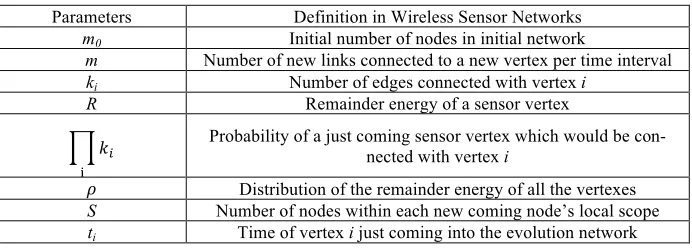
In order to validate the capability of the generated networks with our evolution model, we analyze the evolution results with the connectivity degree distribution. The effect of energy distribution on the connectivity growth of nodes is shown in Figure 1. With different degree distributions, the different mathematical expectations would generate various speeds of connectivity growth.
Fig. 1. Degree of evolution network with different energy distributions
Parameters of the model are R = 1, S = 20, ti = 50, and m = 3 in Figure 1.
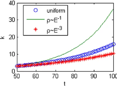
Fig. 2. Degree of evolution network with different local-scopes
Parameters of the model are R = 1, ti = 50, and m = 3 in Figure 2.
Figure 2 shows that the newly coming nodes would select various numbers of ver-texes based on the range of the local-scope. We can see that the smaller S is, the high-er the probability of the node i to be connected.
Fig. 3. Degree of evolution network with different vertex incoming times
Parameters of the model are R = 1, S = 20, and m = 3 in Figure 3.
Figure 3 indicates the effect of a new node's coming time on the connectivity growth. From Figure 3, we can see that the older vertexes have a greater chance of being selected for linking to the new coming vertexes, which means that the connec-tivity of the older vertexes would increase more rapidly than that of the younger.
Fig. 4. Degree distribution with various energy distributions
Parameters of the model are m0 = 5, S = 10, and m = 3 in Figure 4.
From Figure 4, we can see that the degree distribution follows the power-law dis-tribution despite the disdis-tribution of the remainder energy. This means that scale-free WSNs can be obtained by our evolution model in any case.
The above experiments do not take the maximum connectivity constraints ki(max) in-to consideration. After adding the facin-tor inin-to the model, the degree distribution with various energy distributions and the degree of the evolution network with different local-scopes are shown respectively in Figures 5 and 6.
Fig. 6. Degree of network with different local-scopes in modified model
From Figures 5 and 6, we can see that the connectivity speed is much slower be-cause of the maximum connectivity constraints.
4
Conclusions
We have proposed an evolution model for revealing truly the realistic WSNs in this paper. In our model, we added new nodes and links based on the energy-awareness of each sensor node and the energy-balance of the whole network. The simulation results in our experiment have shown that our model is highly compatible with the actual network topology with regards to degree distribution and other critical topology-related metrics.
5
References
[1]Zhang, C. (2010). Cluster-based Routing Algorithms Using Spatial Data Correlation for Wireless Sensor Networks. Journal of Communications, 5(3): 232-238.
https://doi.org/10.4304/jcm.5.3.232-238
[2]Wang, J., Kim, J. U., Shu, L. (2010). A Distance-based Energy Aware Routing algorithm for wireless sensor networks. Sensors, 10(10): 9493-9499. https://doi.org/10.3390/ s101009493
[3]Zhang, D. (2016). Heating Meter Reading System Based on GPRS and Radio Frequency Technology. Revista de la Facultad de Ingeniería, 31(9): 177-185.
[4]Fichera A., Fortuna L., Frasca M., Volpe R. (2015). Integration of complex networks for urban energy mapping, International Journal of Heat and Technology, 33(4), 181-184.
https://doi.org/10.18280/ijht.330423
[6]Zhang, W., Sun, G., Sheng, B. (2015). An Opinion Leaders Detecting Algorithm in Multi-relationship Online Social Networks. International Journal of Hybrid Information Tech-nology, 9(5): 391-398. https://doi.org/10.14257/ijhit.2016.9.5.33
[7]Chua, H. N., Ning, K., Sung, W. K. (2011). Using indirect protein-protein interactions for protein complex prediction. Computational Systems Bioinformatics, 6(3): 97-109.
[8]Sánchezburillo, E., Duch, J., Zueco, D. (2012). Quantum Navigation and Ranking in Com-plex Networks. Scientific Reports, 2: 605-616.
[9]Paparo, G. D., Müller, M., Comellas, F. (2013). Quantum Google in a Complex Network. Scientific Reports, 3: 127-132. https://doi.org/10.1038/srep02773
[10]Tsiotas, D., Polyzos, S. (2015). Decomposing multilayer transportation networks using complex network analysis: a case study for the Greek aviation network. Journal of Com-plex Networks, 3(4): 624-670. https://doi.org/10.1093/comnet/cnv003
[11]Shi, H. S. (2016). A Method of Automatic Detection of Fog Image Based on SVM Classi-fication. Revista de la Facultad de Ingeniería, 31(9): 211-218.
[12]Barabasi, A., Albert, R. (1999). Emergence of scaling in random networks. Science, 286: 509-512. https://doi.org/10.1126/science.286.5439.509
[13]Barabasi, A., Albert, R. (1999). Mean-field theory for scale-free random networks. Phys Rev A, 272(1-2): 173-187. https://doi.org/10.1016/s0378-4371(99)00291-5
[14]Clauset, A., Shalizi, C. R., Newman, J. (2009). Power-Law Distributions in Empirical Da-ta. Siam Review, 4: 661-703. https://doi.org/10.1137/070710111
[15]Mohite, P. (2015). Adaptive Data Fusion for Energy Efficient Routing in Wireless Sensor Network. International Journal of Energy Optimization & Engineering, 4(1): 1-17.
https://doi.org/10.4018/ijeoe.2015010101
[16]Huang, H. P., Chen, J. T., Wang, R. C. (2014). Compressed Sensing Algorithm Based on Data Fusion Tree in Wireless Sensor Networks. Dianzi Yu Xinxi Xuebao/journal of Elec-tronics & Information Technology, 36(10): 2364-2369.
[17]Kumar, L., Ahlawat, M. (2012). Evolution Techniques for Reliability of Wireless Sensor Network. International Journal of Advances in Engineering Sciences, 4: 77-87.
[18]Wang, Q., Chen, J., Fang, H. (2014). Fault-tolerant topology control algorithm for mobile robotic networks. International Journal of Control, Automation and Systems, 12(3): 582-589. https://doi.org/10.1007/s12555-013-0195-5
[19]Miyao, K., Nakayama, H., Ansari, N. (2010). LTRT: An efficient and reliable topology control algorithm for ad-hoc networks, IEEE Transactions on, 12: 6050-6058.
[20]Konstantinidis, A., Yang, K., Chen, H. H. (2007). Energy-aware topology control for wire-less sensor networks using memetic algorithms, Computer Communications, 30(14-15): 2753-2764. https://doi.org/10.1016/j.comcom.2007.05.013
[21]Sehaba, K., Serna, A. (2014). Decoding Social Situations in Adolescents with Asperger through a Serious Game, Modelling, Measurement and Control C, 75(2): 234-247. [22]Semache A., Hamidat A., Benchatti A. (2015). Impact study of the solar energy on the
en-ergy performances of the rural housing in Algeria, International Journal of Heat and Technology, 33(4), 229-236. https://doi.org/10.18280/ijht.330431
[23]Ferentinos, K. P., Tsiligiridis, T. A. (2010). A memetic algorithm for optimal dynamic de-sign of wireless sensor networks, Computer Communications, 2: 250-258.
https://doi.org/10.1016/j.comcom.2009.09.004
[24]Liu, H. R., Yin, W. X., Dong, M. R. (2014). Study on the scale-free topology model with strong intrusion-tolerance ability in wireless sensor networks, Acta Physica Sinica, 63(9): 972-986.
[26]Genco A., Viggiano A., Viscido L., Sellitto G., Magi V. (2016). Numerical simulation of energy systems to control environment microclimate, International Journal of Heat and Technology, 33(S2), S545-S552. https://doi.org/10.18280/ijht.34S249
[27]Liu, H., Yin, R., Liu, B. (2016). A scale-free topology model with fault-tolerance and in-trusion-tolerance in wireless sensor networks, Computers & Electrical Engineering, 56: 533-543. https://doi.org/10.1016/j.compeleceng.2016.01.003
[28]Trancossi M., Pascoa J.C., Xisto C.M. (2016). Design of an innovative off road hybrid ve-hicle by energy efficiency criteria, International Journal of Heat and Technology, 33(S2), S387-S395. https://doi.org/10.18280/ijht.34S228
[29]Chekroun, S., Abdelhadi, B., Benoudjit, A. (2014). A New Approach Design Optimizer of Induction Motor Using Particle Swarm Algorithm, Modelling, Measurement and Control A, 87(2): 89-108.
[30]Puglisi G., Zanghirella F., Ungaro P., Cammarata G. (2016). A methodology for the gener-ation of energy consumption profiles in the residential sector, International Journal of Heat and Technology, 33(3), 491-497. https://doi.org/10.18280/ijht.340320
6
Authors
Hui Gao, majoring in computer application technology, master of engineering,
en-gaged in computer teaching and network R&D, with research focused on computer network and application. He once participated in the national key teacher training and college key laboratory construction and also participated in the provincial project Research on Application of Semiconductor Nanowires in Solar Cells, which was identified as one of the scientific and technological achievements in Henan Province.
Zhixian Yang, majoring in computer application technology, master of
engineer-ing, engaged in computer teaching and software R&D, with research focused on com-puter and IOT application.