International Doctorate School in Information and Communication Technologies
DISI - University of Trento
Distances and Stability
in biological Network Theory
Roberto Visintainer
Advisor:
Dott. Giuseppe Jurman
Fondazione Bruno Kessler
I want to especially thank Kristina Lerman and Steve Horvath and their groups at USC and UCLA who welcomed me and gave me many valuable advices for my Ph.D. work. None of this would have been possible without the friends and colleagues MPBA group at FBK, especially Cesare and Giuseppe who patiently guided me making these last 4 years such an enriching period both professionally and personally.
In this thesis we introduce, define and quantitatively assess the stability of the algorithms for the reconstruction of networks. We will focus on theory, development and implementation of operative procedures and algorithms for the assessment of stability in complex networks for biological systems, with gene regulatory networks as the key example. A major issue affecting network inference is indeed the high variability of network reconstruction and network topology inferred after data perturbation, different parameter choices and alternative methods. Network stability will thus be used to measure reliability of inferred topology, also obtaining confidence intervals for the outcomes. The methods will be employed to introduce a new ap-proach to reproducibility in the study of complex networks. It will also be coupled with statistical machine learning models, in order to integrate fea-ture selection and network inference within a pathway profiling approach. The evaluation of similarity between networks will be the first and central operative procedure of the developed pipelines, the key point being the iden-tification of distances that can compare network structures improving over classical measures based on the confusion matrix, too coarse for this task. A combination of spectral and edit distances especially tailored for biological networks will be investigated and applied to several high-throughput biolog-ical datasets of different nature and with different tasks in oncogenomics, neurogenomics and exposomics.
1 Introduction 1
2 Background and Notation 7
2.1 Networks . . . 7
2.1.1 Definitions . . . 7
2.1.2 Connectivity Matrices . . . 9
2.1.3 Spectrum . . . 12
2.1.4 A minimal example . . . 14
2.2 Biological Networks . . . 16
2.3 Network Inference . . . 21
2.3.1 Weighted Gene Coexpression Network Analysis . . 23
2.3.2 Topological Overlap Matrix . . . 25
2.3.3 Aracne . . . 26
2.3.4 CLR . . . 27
2.3.5 RegnANN . . . 27
2.4 Correlation Measures . . . 32
2.4.1 Pearson . . . 32
2.4.2 Biweight Midcorrelation . . . 32
2.4.3 Maximal Information Coefficient . . . 33
2.5 Resampling Techniques . . . 35
2.5.1 Bootstrap . . . 35
3 Quantitative Network Comparison 39
3.1 Global and Local Distances . . . 40
3.2 Spectral Similarity Measures . . . 42
3.2.1 Benchmarking Experiments . . . 47
3.2.2 Data Description . . . 47
3.2.3 Results . . . 51
4 HIM, Hamming - Ipsen-Mikhailov Distance 59 4.1 Definition . . . 59
4.2 A Biological Example . . . 63
4.3 Module Preservation . . . 65
4.3.1 Data . . . 66
4.3.2 Results . . . 69
5 Stability 77 5.1 Stability indicators . . . 77
5.2 Reproducibility In Network Inference and Analysis . . . . 80
5.2.1 FDR effect on correlation networks . . . 80
5.3 Inference Methods Comparison on Synthetic Data . . . 87
5.3.1 Synthetic Data . . . 88
5.3.2 Escherichia Coli Data . . . 91
6 Differential Networking 99 6.1 Biological Network Comparison: a miRNA example . . . . 99
6.2 Sources of Variability in Pathway Profiling . . . 106
6.3 HIM Framework on Biological datasetata . . . 109
6.3.1 Children susceptibility to air pollution . . . 109
6.3.2 Alzheimer’s Disease . . . 115
6.3.3 Parkinson’s Disease . . . 125
Bibliography 143
A Module Preservation: Measures and Results 165
A.1 Module Preservation Measures . . . 165
A.2 Statistics for module quality assessment . . . 170
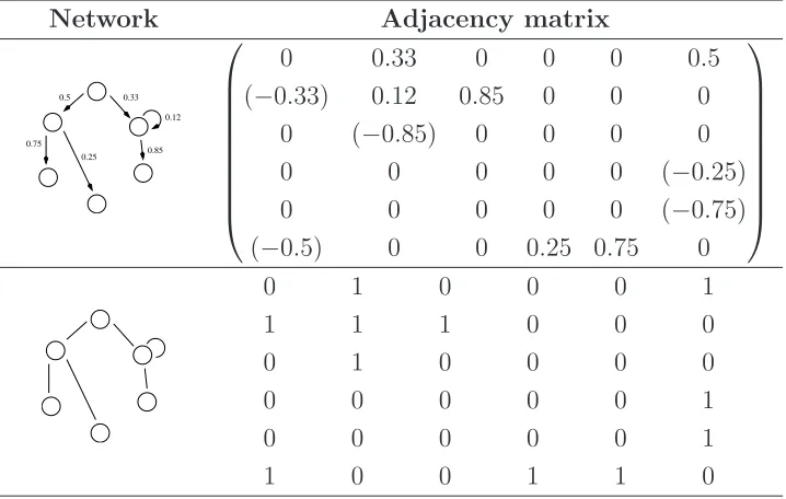
2.1 Adjacency matrices for the weighted directed network can be written in two alternative ways (1) with sign indicating direction (2) asymmetric, with the (positive) value only in
the entry (i, j) to represent the connectioni →j, see Fig.2.1
and its topology; nodes ordering is clockwise starting from
the top node. . . 9
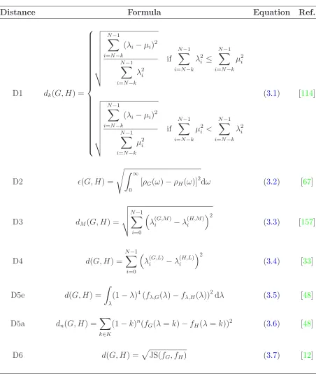
3.1 Spectral graph distances . . . 48
3.2 Number of links in the original matrix A, in the fully
con-nected matrix F (maximum number of links for the given
dimension) and in the perturbed matrix A5, expressed as
mean ± standard deviation on 50 replicates. . . 49
3.3 Results of the experiments on the first benchmarking dataset.
For each measure D1-D6 and number of network verticesN,
we report the values of the distances between the network
A and the networks A5, A and F in terms of the minimum
(m), mean (µ) ± standard deviation and maximum (M) on
the 50 replicates. Values of D5 are in 10−3. . . 51
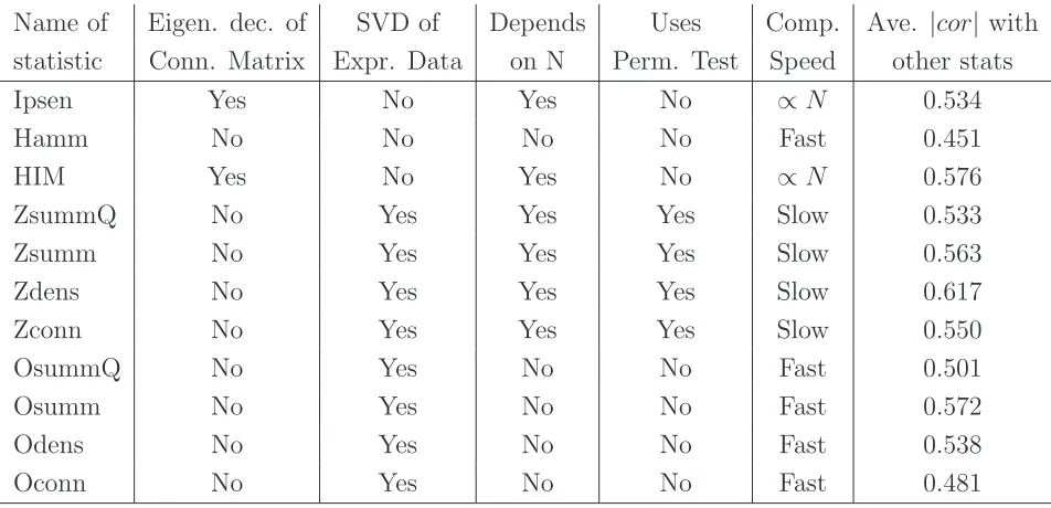
4.1 Statistics Description Summary . . . 67
4.2 Mean and Standard Error of Spearman correlations across
5.1 Statistics (mean, bootstrap confidence intervals and range)
of the stability indicators I1 and I2 for different instances of
the WGCNA and MIC networks on the dataset S and for
different values of data subsampling. . . 85
5.2 Top ranked links, ordered by weight range over weight mean
across all 20 resampling ofk4 4-fold cross validation, for the
three algorithms WGCNA, WGCNAFDR1e-4 and MIC . . 93
5.3 Top ranked nodes, ordered by degree range over degree mean
across all 20 resampling ofk4 4-fold cross validation, for the
three algorithms WGCNA, WGCNA FDR 1e-4 and MIC.
(*) indicates that Ratio and Mean are both zero. . . 94
6.1 Statistics (mean, bootstrap confidence intervals and range)
of the stability indicators I1 and I2 for the CLR inferred
networks on the datasets MT, MnT, FT, FnT, for different
values of data subsampling. . . 102
6.2 Position in the weight Range/Mean ranking in the four cases
MT, MnT, FT, FnT for six miRNA-miRNA links. . . 103
6.3 Air Pollution Experiment: pathways corresponding to mostly
discriminant genesg1, ..., gk ranked by the normalized
Ipsen-Mikhailov distance ˆǫ. The number of genes belonging to the
pathway is also provided. . . 111
6.4 Air Pollution Experiment: list of Agilent probesets in the
signature with their corresponding Entrez Gene Symbol ID and GO pathway. The list is ranked according to the
de-creasing absolute value of the differential node degree ∆d. 112
by the normalized Ipsen-Mikhailov distance ˆǫ. The Entrez gene symbol ID is also provided for the selected probesets
g1, ..., gk in the corresponding pathway. . . 113
6.6 AD: most important pathways ranked by normalized
Ipsen-Mikhailov distance ˆǫ. The Entrez gene symbol ID is also
pro-vided for the selected probesets g1, ..., gk in the
correspond-ing pathway. In bold, common pathways between early and
late stage AD. . . 117
6.7 AD Experiment: selected pathways for early (left) and late
(right) stage corresponding to mostly discriminant genes
g1, ..., gk ranked by the normalized Ipsen-Mikhailov distance
ˆ
ǫ. The number of genes belonging to the pathway is also
provided. In bold, the common pathways. . . 121
6.8 AD Experiment (early): list of Affymetrix probesets in the
early stage signature with their corresponding Entrez Gene Symbol and GO pathway. The list is ranked according to the decreasing absolute value of the differential node degree
∆d. . . 123
6.9 AD Experiment (late): list of Affymetrix probesets in the
late stage signature with their corresponding Entrez Gene Symbol and GO pathway. The list is ranked according to the decreasing absolute value of the differential node degree
6.10 Number (n)m of pathways found for the network inference
step for different combinations of model M,
knowledge-base D, and enrichment E. n: all networks (unfiltered);
m: filtered networks, having more than 5 and less than
1000 genes on HG-U133A with non-null intra-class
vari-ance. Intersections ℓL, E3∩ and E2∩ are respectively
de-fined as ℓL := ℓ1ℓ2 ∩ Liblinear, E2∩ := WebGestalt∩ PaLS,
E3∩ := WebGestalt∩GSEA∩PaLS. . . 126
6.11 Summary of most disrupted pathways retrieved by WebGestalt
and PaLS. . . 128
6.12 Summary of GO terms in MDPs common between WG and
PaLS, for both M models. GO terms are sorted for
de-creasing HIM median (computed overE and N). Bold fonts
identify the GO terms shared by models. . . 139
6.13 Summary of KEGG pathways in MDPs common between
WebGestalt and PaLS, for both M models. KEGG
path-ways are sorted for decreasing HIM median (computed over
E and N). Bold fonts identify the KEGG pathways shared
by models M. . . 139
A.1 Preservation of female mouse liver modules in male data ref
1 test 2 (corr method: Spearman) . . . 171
A.2 Preservation of human brain modules in chimpanzee brains
and vice versa ref 1 test 2 (corr method: Spearman) . . . . 172
A.3 Preservation of human brain modules in chimpanzee brains
and vice versa ref 2 test 1 (corr method: Spearman) . . . . 172
A.4 Preservation of KEGG pathways between human and chimp
data ref 1 test 2 (corr method: Spearman) . . . 175
data ref 2 test 1 (corr method: Spearman) . . . 176
A.6 Preservation of Cholesterol Biosynthesis Process module among 8 tissue/gender combinations in F2 mice (corr method:
Spear-man) . . . 176
A.7 Correlation between Mod.Ipsen distance and the Network-based module preservation measures for each tissue used as Reference (corr method: Spearman). Missing values are due
to zero standard deviation in the considered values . . . . 177
A.8 Correlation between Mod.Ipsen distance and the Network-based module preservation measures for each tissue used as Test (corr method: Spearman). Missing values are due to
2.1 Network types . . . 8
2.2 Examples of Cauchy-Lorentz distributions with different
pa-rameters. . . 14
2.3 Adjacency matrix and graphical representation of I1 . . . . 15
2.4 Adjacency matrix and graphical representation of I2 . . . . 16
2.5 Lorentzian distribution of the Laplacian spectra for I1 and
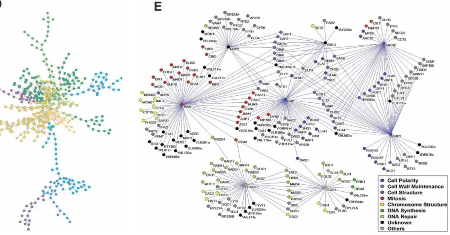
2.6 Examples of the five major biological networks. (A) A yeast transcription factor-binding network, composed of known transcription factor-binding data collected with large-scale ChIPchip and small-scale experiments. This figure was
gen-erated with the program Pajek [39]. (B) A yeast
proteprotein interaction network, containing proteproteinproteprotein in-teractions identified by yeast two-hybrid and protein com-plexes identified by affinity purification and mass
spectrom-etry [17]. (Reprinted by permission from Macmillan
Pub-lishers Ltd: Nature [69], 2001.) Nodes are colored
accord-ing to the mutant phenotype. (C) A yeast tion network comprised primarily of in vitro
phosphoryla-tion events identified using protein microarrays [117]. The
figure was generated with Osprey 1.2.0. [25]. (D) An E.Coli
metabolic network with 574 reactions and 473 metabolites colored according to their modules (Reprinted by permission
from Macmillan Publications Ltd: Nature [58], 2005). (E)
A yeast genetic network constructed with synthetic lethal interactions using SGA analysis on eight yeast genes (From
[139]; reprinted with permission from AAAS). Nodes are
col-ored according to their YPD cellular roles [taken from [158]]. 20
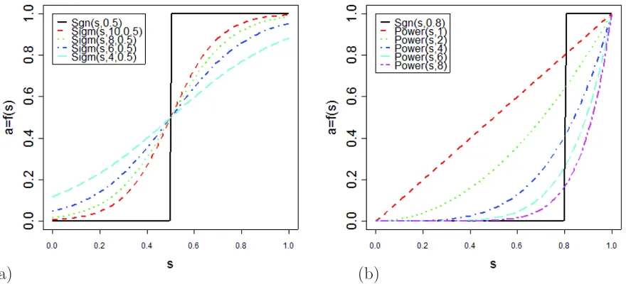
2.7 Adjacency functions for different parameter values. a)
Sidg-moid and signum adjacency functions. b) Power and signum adjacency functions. The value of the adjacency function (y-axis) is plotted as a function of the similarity (co-expression measure). Note that the adjacency function maps the
inter-val [0,1] into [0,1]. [61, 154] . . . 23
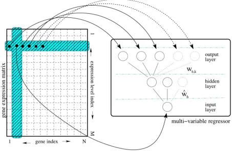
put/output patterns starting from a gene expression ma-trix.Each input pattern corresponds to the expression value
for the selected gene of interest. . . 28
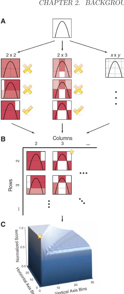
2.9 Computing MIC (A) For each pair (x, y), the MIC algorithm
finds the x-by-y grid with the highest induced mutual
infor-mation. (B) The algorithm normalizes the mutual informa-tion scores and compiles a matrix that stores, for each res-olution, the best grid at that resolution and its normalized score. (C) The normalized scores form the characteristic ma-trix, which can be visualized as a surface; MIC corresponds to the highest point on this surface. In this example, there are many grids that achieve the highest score. The star in (B) marks a sample grid achieving this score, and the star in (C) marks that grid’s corresponding location on the surface.
[taken from [120]] . . . 34
3.1 Representation of the physical network model of D2 distance. 43
3.2 Benchmark Dataset B1(b,25,5): the original graph A, the
perturbed graphA5, the complemental graphAand the fully
connected graph F. . . 49
3.3 Benchmark DatasetsB2(b,20,25,5) (upper row) andB3(b,20,25,5,5)
(lower row): the original graph S1 (first element of the
se-ries), the tenth element S10 of the series and the final graph
S20. . . 50
3.4 Plots of the distances of consecutive elements of the series for
the dataset B2(50,25,5). Solid line: mean over the b = 50
replicates; dashed lines: minimum and maximum over the
3.5 Mutual scatterplots (upper triangle) and correlation values
(lower triangle) for the Exp. 2. . . 53
3.6 Plots of the distances of consecutive elements of the series
for the dataset B3(50,25,5,5). Solid line: mean over the
b = 50 replicates; dashed lines: minimum and maximum
over the b = 50 replicates. . . 55
3.7 Mutual scatterplots (upper triangle) and correlation values
(lower triangle) for the Exp. 3. . . 56
3.8 Cluster dendrograms with average linkage and correlation
distance of D1-D6 for the two Experiments 2 and 3. . . 57
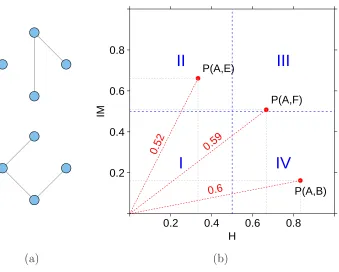
4.1 An example of HIM distance. (a) Network A (top) and
Net-work B (bottom); (b) Representation of the HIM distance in the Ipsen-Mikhailov and Hamming distance space between networks A versus B, E and F, where F is the fully connected
network and E is the empty one. . . 62
4.2 (a) Evolution of distances of the D. melanogaster network
time series in the Hamming/Ipsen-Mikhailov space and (b) evolution of glocal distances of the D. melanogaster network along 66 time points in the 4 stages Embryonic (E), Larval
(L), Pupal (P) and Adult (A) . . . 64
thesis gene module in the considered mouse tissues.
The module is here represented as a weighted signed cor-relation network where the nodes represent the genes from the GO category Cholesterol Biosynthetic Process. Module preservation techniques applied here allow the assessment of the similarity between these networks. Here we represent the connectivity pattern between the cholesterol biosynthe-sis genes in 4 different tissues from male and female mice. The thickness of the link represents the absolute value of correlation, while the colors red and green show positive correlation or anticorrelation respectively. The dimension of the nodes is proportional to their connectivity values, so the hubs of the module are represented by larger circles. This kind of plot shows how across the tissues there is a high resemblance between the module in male and female
samples. . . 72
4.4 Preservation Measures: a) Median Rank, b) Zsummary, c)
HIM based (1-HIM). 12 modules detected in female liver
data in a Modul Size vs. Preservation plot. . . 73
4.5 A) HIM Preservation of the cholesterol pathway between the
tissues. Z Summary Preservation of the cholesterol pathway between the tissues. B) On rows are presented the reference
4.6 Correlation between measures of female mouse liver module preservation in male data. Correlation between the preservation measures of the 12 modules computed with
the analized methods (Ipsen-Mikhailov (ǫ), Hamming (H),
HIM (φ),ZsummaryQuality,ZsummaryP reservation,Zdensity,Zconnectivity,
medianRanksummaryQuality,medianRanksummaryP reservation,medianRankdensity,
medianRankconnectivity). Considering the plot as a matrix,
lower triangular elements are depicted a pairplot for each couple of measures. Each circle represents one of the mod-ules detected with WGCNA. On the diagonal we present a barplot of the distribution of the measures for each method. The upper triangular part of the plot reports the values for
Spearman correlation. . . 75
5.1 Scheme of a resampling framework applied on a dataset D
made by p features and s samples. In this example the
number of folds is r so that each subsample training set is
made by n samples. r needs to be smaller than s choose n. 79
5.2 The correlation matrix MS used to generate the synthetic
dataset S . . . 82
5.3 Correlation networks inferred by the dataset S using (a)
absolute Pearson, (b) absolute Pearson with FDR correction
at p-value 10−4 and (c) MIC. Node label i corresponds to
feature fi, node size is proportional to node degree and link
colors identify different classes of link weights. . . 83
5.4 I1 andI2 stability indicators (mean and confidence intervals)
for different instances of the WGCNA and MIC networks on
the dataset S and for different values of data subsampling. 84
5 regulators, 42 links). . . 89
5.6 The effect of different FDR settings on accuracy and
sta-bility of network inference performed with correlation and
bicorrelation. . . 90
5.7 Performances of the 9 inference algorithm tested on
syn-thetic dataset computed ad HIM distance from the gold
standard (GS). FDR=10−4 . . . 91
5.8 A subnetwork ofEscherichia Coli consisting of 50 nodes and
their 102 connections; in particular notice the connections
involving the 5 regulators (arcA, rutR, gadE, gadX, gadW). 95
5.9 The effect of different FDR settings on accuracy and
sta-bility of network inference performed with correlation and
bicorrelation. . . 96
5.10 Performances of the 9 inference algorithm tested on the
E.Coli subnetwork dataset computed ad HIM distance from
the gold standard (GS). FDR=10−4 . . . 97
6.1 Mutual HIM distances for the four CLR inferred networks
MT, MnT, FT, FnT reconstructed from the whole corre-sponding subsets and correcorre-sponding 2D multidimensional
scaling plot. . . 101
6.2 CLR networks (and corresponding density values) inferred
from the 4 subsets (a) Male Tumoral (MT) (b) Male not Tumoral (MnT) (c) Female Tumoral (FT) and (d) Female
non Tumoral (FnT) of the datasets HCC. Links are
thresh-olded at weight 0.1, node position is fixed across the four networks, node dimension is proportional to the degree and
6.3 I1 andI2 stability indicators (mean and confidence intervals)
of CLR inferred networks for different values of data sub-sampling on the four subgroups Male Tumoral (MT), Male not Tumoral (MnT), Female Tumoral (FT) and Female non
Tumoral (FnT) of the datasets HCC. . . 105
6.4 The general scheme of the HIM framework. Algorithms and
tools used in the PD study are listed in ovals. . . 106
6.5 Networks of the pathway GO:0007399 (nervous system
de-velopment) for Prachatice children (a) compared with Teplice
children (b). Node diameter is proportional to the degree, and edge width is proportional to connection strength
(esti-mated correlation). . . 114
6.6 Networks of the pathway GO:0019787 for AD early
develop-ment patients (a) compared with healthy subjects (b). Node diameter is proportional to the degree, and edge width is
proportional to connection strength (estimated correlation). 116
6.7 GO subgraphs for Alzheimer’s early and late stage
(Molec-ular Function and Biological Processes domains). Selected nodes are represented in light gray, gray and dark gray for
late, early and common nodes. . . 122
6.8 HIM maps for all combinations of M,D,E and N. Subplot
(c) is reproduced in the main paper as Figure 6.8(d). . . . 129
6.9 Distance distribution for N = Aracne and D = GO (all
enrichment methods and all models). (a) Distribution of the
HIM distance. Gray line: kmeans centroids (HIM ≈ 0.056
and HIM ≈ 0.247). Red line: chosen threshold HIM ≈
0.152, equidistant from the two centroids. (b) HIM map of
the two centroids. Red line: HIM = 0.15. . . 130
HIM maps distance for different E methods. Red line corre-sponds to threshold HIM = 0.15 separating two clusters. (b)
Histograms of pathway cardinality below and above threshold.131
6.11 HIM plots for M = Liblinear and D = KEGG, for all
en-richment methods. Symbols indicate enen-richment methods: Aracne (squares), CLR (circles), WGCNA (triangle). Red
line: the threshold τ = 0.05 defining MDPs. (a) HIM maps
grouped by E. Each pathway is inferred by the three
meth-ods N as detailed in the legend on top of the figure. (b)
Trellis displays for histogram plots of HIM distance distri-bution conditioned for WebGestalt and PaLS and the three
subnetwork inference algorithms N. . . 132
6.12 Network analysis of the ALS KEGG pathway (as defined by
PALS). (a-b): Networks were separately inferred by WGCNA for the PD patients (a) and controls (b). The networks are thresholded at edge weight 0.5 for graphic purposes. Node labels represent Entrez IDs. (c): Boxplots of the HIM
stabil-ity distribution (m = 100 replicates as defined in Subsection
4.1) comparing PD patients and controls separately for the
3 inference methods N. (d): HIM map of all m comparisons.135
6.13 Variability of networks on the ALS KEGG pathway,
de-fined by PALS, inferred by WGCNA on PD samples, for
m=100 replicates and 2/3 resampling. The two network
in-stances have (a) smallest HIM and (b) largest HIM from the network inferred on all samples (shown in the main
pa-per, Fig: 6.11(a)). Only links of weight > 0.5 are displayed.
6.14 Leave-One-Out stability of the ALS KEGG pathway (as de-fined by PALS). (a): Boxplots of the Leave-One-Out HIM stability distribution comparing PD patients and controls
separately for the 3 inference methods N. (b): HIM map of
all m+1 and m−1 comparisons. Different colors are used for
the three N. . . 137
6.15 Network analysis of the Pathogenic E. coli infection KEGG
pathway (as defined by PALS). (a-b): Networks were sepa-rately inferred by WGCNA for the PD patients (a) and con-trols (b). The networks are thresholded at edge weight 0.5 for graphic purposes. Node labels represent Entrez ID. (c):
Boxplots of the HIM stability distribution (m = 100
repli-cates as defined in the main paper, Subsection 2.1) compar-ing PD patients and controls separately for the 3 inference
methods N. (d): HIM map of all m comparisons. Different
colors are used for the three N. (e): Boxplots of the HIM
Leave-One-Out stability distribution comparing PD patients
and controls separately for the 3 inference methods N. (f):
HIM map of all m+1 and m−1 comparisons. Different colors
are used for the three N. . . 138
A.1 A) Preservation of human brain modules in chimpanzee brains (corr method: Spearman). B) Preservation of chimpanzee
brain modules in human brains (corr method: Spearman) . 173
A.2 A) Preservation of KEGG pathways between human and chimpanzee data using human as reference and chimp as test (corr method: Spearman). B) Preservation of KEGG pathways between human and chimpanzee data using chimp
as reference and human as test (corr method: Spearman) . 174
8 tissue/gender cobinations in F2 mice (corr method:
Introduction
Reproducibility, i.e., the possibility of independently repeating a suite of
experiments obtaining the same (or very similar) outcome of the original study, is a key ingredient of the scientific method. In the last few years, the need for reproducibility has become a major task also in very young disciplines such as computational biology and bioinformatics, where the relevant impact of noise and the paucity of data represent daily obstacles to overcome in warranting a completely reproducible pipeline to be set and
shown [66, 138]. Among the several aspects included under the umbrella
CHAPTER 1. INTRODUCTION
complexity-aware overview of the net of their mutual relations, the amount of research activities aimed at reconstructing such networks from various
biological signals has skyrocketed in the last decade [16]. Moving even one
step further, the concept of stability as the continuous dependence of the inference algorithm result from perturbations of the original data is of par-ticular interest because of the ever growing diffusion of two novel research directions stemming from the network reconstruction theory. The former is the differential network analysis methods, where the emphasis of detecting the features discriminating two conditions or two phenotypes is moving
form the gene to the pathway (and thus the network) level [65, 31] and
the latter is the integration of the biological network with socioeconomic and contact networks describing people’s behavior in order to construct a
brand new network medicine approach [95, 16].
As anticipated in the previous paragraph, the problem of inferring a biolog-ical network structure starting from a set of high-throughput measurements
(e.g. gene expression arrays or digital gene expression from Next
Gener-ation Sequencing data) has been positively answered by a huge number of deeply different solutions published in the literature in the last fifteen years, ranging from purely deterministic (algebraic or analytic) to purely probabilistic (Bayesian). In this thesis, we also propose a novel reconstruc-tion method (called RegnANN) based on artificial neural networks, which
we prove to be a good compromise between performance and stability [56].
Nonetheless, network reconstruction suffers from being a underdetermined problem, being the number of interactions highly larger than the number
of independent measurements [40]: thus any algorithm has to look for a
compromise between accuracy and feasibility, allowing simplifications that inevitably mine the precision of the final outcome, for instance including
a relevant number of false positive links [76]. This makes the inference
problem ”a daunting task” [18], not only in terms of devising an effective
algorithm, but also in terms of quantitatively interpreting the obtained results. In general, the reconstruction accuracy is far from being optimal
in many situations with the presence of several pitfalls [103], related to
both the methods and the data [60], with the extreme situation of many
link prediction being statistically equivalent to random guesses [116]. In
particular, the size (and the quality) of the available data play a critical
role in the inference process, as widely acknowledged [94, 53, 105]. All
these considerations support deeming network reconstruction a still
un-solved problem [135].
Despite the ever rising number of available algorithms, only recently ef-forts have been carried out towards an objective comparison of network
inference methods also highlighting current limitations [4, 83] and relative
strengths and disadvantages [98]. Among those, it is worthwhile
men-tioning the international DREAM challenge [100], whose key result in the
last edition advocated integration of predictions from multiple inference methods as an effective strategy to enhance performances taking
advan-tage from the different algorithms’ complementarity [40]. Nevertheless,
CHAPTER 1. INTRODUCTION
data would generate different networks. Thus, in the spirit of applying reproducibility principles to this field, one has to accept the compromise that the inferred/non inferred links are just an estimation, lying within a reasonable probability interval. In brief, we aim at proposing a set of four indicators allowing the researcher to quantitatively evaluate the reliability of the inferred/non-inferred links. In detail, we quantitatively assess, for a given ratio of removed data and for a give number of resampling, the mutual distances among all inferred networks and their distances to the network generated by the whole dataset, with the idea that, the smaller the average distance, the stabler the network. Moreover, we provide a ranked list of the stablest links and nodes, where the rank is induced by the variability of the link weight and the node degree across the generated networks, the less variable being the top ranked.
Last but not least, thorough the whole stability pipeline the major ingredi-ent is represingredi-ented by availability of a consistingredi-ent network metric expressing the distance between two graphs sharing the same nodes but a different wiring. The part of network theory dealing with the assessment of the sim-ilarity of two networks is called network comparison. Comparison methods are essential with dynamic networks to measure differences between two consecutive network states and then model the whole series, for instance when investigating the changes of a protein-protein interaction network during a biological process such as a disease. The theory of network com-parison is based on the variety of similarity measures, whose taxonomy is essentially parted into two major branches: the indirect methods of feature-based measures and the direct methods making use of a suitable distance. Although fruitful insights can be drawn by indirect methods, a distance must be employed whenever a quantitative assessment of the differences between two elements is required. Traditional choices are members of the family of the edit distances, where the minimum number of link operations
(deletion and insertion) for transforming one topology into the other is evaluated, and the family of spectral distances, where the difference of the eigenvalues distribution of one the connectivity matrices of the networks is taken into account. To cope with the different pros and cons of both edit
and spectral similarity, we propose here the HIM distance [75] which is the
product metric of the spectral Ipsen-Mikhailov and the edit Hamming dis-tance: the HIM distance is the base of the whole aforementioned stability framework.
Biological applications of the HIM distance and of the stability indicators are shown in the last chapter, where a number of tasks in exposomics, oncogenomics and neurogenomics are presented and discuss, as examples of how these newly introduced algorithms can be an effective tools for the researcher in the network branch of the systems biology.
CHAPTER 1. INTRODUCTION
Background and Notation
The representation of complex systems in terms of networks allows the formalization of the system agents and their interactions. By means of the properties of the underlying graph it is possible to describe and analyze the system itself. For instance the study of the power supply system of a big city using network theory could give insights about weakness points in the system and avoid possible failures.
2.1
Networks
2.1.1 Definitions
Any network can be formally represented as a mathematical entity called
graph. A graph consists of a number N of nodes, also called vertices that
can be finite or infinite and E edges, links or arrows that connect a couple
of vertices representing an interaction (N ∈ N{∞}). For any network G,
its topology consists of the set V(G) = {v1, ..., vn} of its nodes and the
set E(G) = {e1 = (vi1, vj1),· · ·eE = (viE, vjE)} of its edges, neglecting here weights and directions. Different types of graph sharing the same topology
2.1. NETWORKS CHAPTER 2. BACKGROUND AND NOTATION
0.25 0.75
0.5 0.33
0.12
0.85
0.25 0.75
0.5 0.33
0.12
0.85
Weighted digraph Unweighted digraph Weighted graph Underlying topology
Figure 2.1: Network types
and y we say that they are neighbors, we can identify a set of neighbors
for each node.
Links can be bidirectional or unidirectional, this basic feature determining
whether the graph is
• directed (digraph): contains exclusively unidirectional links
• undirected: contains exclusively bidirectional links
• mixed: can contain both unidirectional and bidirectional links. Graphically edges are depicted as arrows to symbolize directed links, lines or double-headed arrows for undirected ones. Only undirected graphs will be used hereafter. From the definition of graph it follows that any link can connect two nodes, but also a self connection is possible: an edge from a
vertex to itself originates a loop in the network. Another feature of the
interactions that can be carried by the edges is their intensity or weight, in this case we have a weighted network. For instance the weight of a link could be used to convey the information about the number of passengers moving from an airport to another in a transportation network. Formally,
a weighted network G(V, E, W) can be formalized as a graph in which links
(x, y) are associated to a number called weight of the link w(x, y) so that
if w(x, y) = 0 then (x, y) ∈/ E and w(x, y) 6= 0 if w(x, y) ∈ E.
Table 2.1: Adjacency matrices for the weighted directed network can be written in two alternative ways (1) with sign indicating direction (2) asymmetric, with the (positive) value only in the entry (i, j) to represent the connection i → j, see Fig. 2.1 and its topology; nodes ordering is clockwise starting from the top node.
Network Adjacency matrix
0.25 0.75
0.5 0.33 0.12 0.85
0 0.33 0 0 0 0.5
(−0.33) 0.12 0.85 0 0 0
0 (−0.85) 0 0 0 0
0 0 0 0 0 (−0.25)
0 0 0 0 0 (−0.75)
(−0.5) 0 0 0.25 0.75 0
0 1 0 0 0 1
1 1 1 0 0 0
0 1 0 0 0 0
0 0 0 0 0 1
0 0 0 0 0 1
1 0 0 1 1 0
2.1.2 Connectivity Matrices
A widely used way to represent graphs is by means of matrices especially
the adjacency matrix.
Adjacency Matrix
The adjacency matrix A is defined as an N ×N squared matrix in which
each entry aij corresponds to the link between the nodes i and j. In
particular, for an unweighted link aij will be 1 when the link is present
((i, j) ∈ V) and 0 otherwise, see 2.1.
A is a very important and useful tool in graph theory, it is in fact enough
to understand many of its basic topological characteristics.
• If A is symmetric, i.e. A(h, k) = A(k, h)∀h, k ∈ V, then the graph is
2.1. NETWORKS CHAPTER 2. BACKGROUND AND NOTATION
• If the diagonal of A has all entries equal to 0, i.e. A(h, h) = 0∀h ∈
1, ..., n there are no self-loops in the graph.
For a weighted link we can define a the matrix of weights of G as W =
(w(x, y))x,y∈V. The weights matrix can alone completely describe the
topol-ogy and the characteristics of a graph, in this case we talk about weighted
adjacency matrix as shown in 2.1. If A is in the form: A = 0 B
BT 0
!
,
where B is a p×q matrix, we have a bipartite graph, a graph in which
the nodes can be classified into two groups N1 with |N1| = p and N2 with
|N2| = q. A link (i, j) exists if and only if i and j belong to different
groups. Another specific configuration of A is the block diagonal matrix:
A = B1 0
0 B2
!
, where B1 and B2 are p× p and q × q matrices
respec-tively. Also in this case we have a subdivision of the nodes into two groups
N1with|N1| = p and N2with|N2| = q, but the links connect exclusively
couples of nodes belonging to the same group forming two separate sub-graphs. This kind of adjacency matrix, where the groups of nodes are in
general upper bounded by the number of nodes, is called disconnected
graph.
The entries in the diagonal aij can be different from zero if selfloops are
allowed; if no self-loops occur we call the graph simple: thus simple graphs
have adjacency metric with zero diagonal. In Table 2.1 we show two
exam-ples of adjacency matrices for two graphs whose representation reads the nodes clockwise starting from the top one. In general a graphical represen-tation is not unique, in the sense that it depends on the actual labeling of the nodes and isomorphic graphs (identical graphs with permuted labels) share the same adjacency matrix. Similarly, graphical representations are not unique too, since node placement is arbitrary.
Degree
The degree of a node is a concept of crucial importance in graph theory since it is the measure of level of interaction of the node with its neighbors
and consequently with the whole network. We define the out-degree
dout(x) as the number of links that exit from node x. Similarly we refer
to in-degree din(x) as the number of links that point to x. Both the
previous definitions are applied to directed graphs: for undirected graph
the in- and out-degree coincide and thus the degree d(x) indicates the
number of links touching the node x itself. Following this definition for the
majority of the authors the self loops are counted twice. We also define
the N×N degree matrix D as the diagonal matrix with the degree of each
node as entries. For instance the degree matrix of the bottom network in
Table 2.1 is D =
2 4
1 1
1 3
.
Theweighted degree (also calledstrength) of a node xin an undirected
network is defined as the sum of the weights of all the links touching x, so
we have that s(x) =P
y∈V w(x, y) where V is the set of neighbors of x.
Laplacian Matrix
The Laplacian matrix L of a graph is defined as the difference between the
degree matrix and the adjacency matrix L = D −A. From the definition
follows that for an unweighted undirected graph without loops (a simple
graph), the sums of the rows and the columns of L are zero.
Two normalizations of the Laplacian matrix exist L = D−1/2LD−1/2 =
2.1. NETWORKS CHAPTER 2. BACKGROUND AND NOTATION
D−1/2 is the diagonal matrix with entries −√δij
degj
. Their entries can explic-itly written as:
L =
1 if i = j and degi 6= 0
−√deg1
idegj
if ij is an edge
0 otherwise
∆ =
1 if i = j and degi 6= 0
−deg1j if (i, j) ∈ V is an edge
0 otherwise
Other kinds of networks have been described in the literature, but will not be used here. In labeled graphs, nodes are classified by functions from some subsets of the integers to the vertices or edges. Hypergraphs instead are characterized by links that can connect any number of vertices, while in multigraphs a couple of nodes can be connected by any number of links.
2.1.3 Spectrum
The eigenvalues of a matrix M ∈ Cn×n are the n roots of its characteristic
polynomialp(z) =det(zI−M). The set of these roots is called thespectrum
and is denoted by λ(M). If λ(M) = λ1, . . . , λn then it follows that
det(a) = λ1, λ2,· · · , λn.
Moreover, if we define the trace of A by
tr(A) =
n
X
i=1
aii
then the tr(A) =λ1 +· · ·+λn. this follows by looking at the coefficient of
z in the characteristic polynomial.
If λ ∈ λ(A) then the nonzero vectors x ∈ Cn that satisfy
Ax = λx
are referred to aseigenvectors. More precisely, x is aright eigenvector for λ
if Ax = λx and a left eigenvector if xHA = λxH. Unless otherwise stated,
“eigenvector” means “right eigenvector” [55].
An undirected and unweighted graph has symmetric real connectivity ma-trices and therefore real eigenvalues and a complete set of orthonormal eigenvectors. Also, for each eigenvalue, its algebraic multiplicity coincides
with its geometric multiplicity. Since A has zero diagonal, its trace and
hence the sum of the eigenvalues is zero. Moreover, L is positive
semidefi-nite and singular, so the eigenvalues are 0 =µ0 ≤ µ1 ≤ · · · ≤µn1 and their
sum (the trace of L) is twice the number of edges. Finally, the eigenvalues
of L lie in the range [0,2]. While the connectivity matrices depend on the
vertex labeling, the spectrum is a graph invariant. Two graphs are called isospectral or cospectral if the corresponding connectivity matrices of the graphs have equal multisets of eigenvalues. Isospectral graphs need not be isomorphic, but isomorphic graphs are always isospectral. Moreover it can be proved that the spectrum of the adjacency matrix of a bipartite graph
is symmetric with respect to 0, i.e. if α is an eigenvalue of A then also −α
is an eigenvalue. Network classification in terms of their spectrum is still
an open problem [144, 150, 151]: however, a first attempt to (qualitative)
network classification in terms of graph spectra can be found in [12, 13] by
Banerjee.
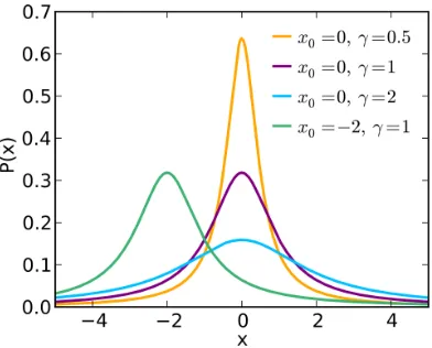
Cauchy-Lorentz distribution
The Cauchy-Lorentz distribution is a continuous probability distribution with probability distribution function PDF given by:
f(x;x0, γ) =
1
π
γ
(x−x0)2 + γ2
2.1. NETWORKS CHAPTER 2. BACKGROUND AND NOTATION
where x0 indicates the peak of the distribution (also called the mode)
of the distribution, and γ specifies half the width of the PDF at half the
maximum height: see the graphical trend of the Cauchy Lorenz distribution
in Figure 2.1.3.
Figure 2.2: Examples of Cauchy-Lorentz distributions with different parameters.
2.1.4 A minimal example
Consider the two networks I1, I2 ∈NNN with corresponding adjacency
matri-ces AI1
, AI2
shown in Fig. 2.3 and 2.4.
The corresponding Laplacian matrices and eigenvalues are
LI1
=
3 −1 0 0 −1 0 0 −1
−1 3 0 0 0 0 −1 −1
0 0 2 0 0 −1 −1 0
0 0 0 2 −1 −1 0 0
−1 0 0 −1 2 0 0 0
0 0 −1 −1 0 2 0 0
0 −1 −1 0 0 0 3 −1
−1 −1 0 0 0 0 −1 3
spec(LI1
) = 0
0.657077
1
2.529317
3 4 4
4.813607
AI1 =
0 1 0 0 1 0 0 1 1 0 0 0 0 0 1 1 0 0 0 0 0 1 1 0 0 0 0 0 1 1 0 0 1 0 0 1 0 0 0 0 0 0 1 1 0 0 0 0 0 1 1 0 0 0 0 1 1 1 0 0 0 0 1 0
0 1 2 3 4 5 6 7
Figure 2.3: Adjacency matrix and graphical representation of I1
LI2
=
3 −1 0 0 0 −1 −1 0
−1 3 0 0 −1 −1 0 0
0 0 0 0 0 0 0 0
0 0 0 2 0 0 −1 −1
0 −1 0 0 1 0 0 0
−1 −1 0 0 0 2 0 0
−1 0 0 −1 0 0 3 −1
0 0 0 −1 0 0 −1 2
spec(LI2
) = 0 0
0.340321
1.145088
3 3
3.854912
4.659679
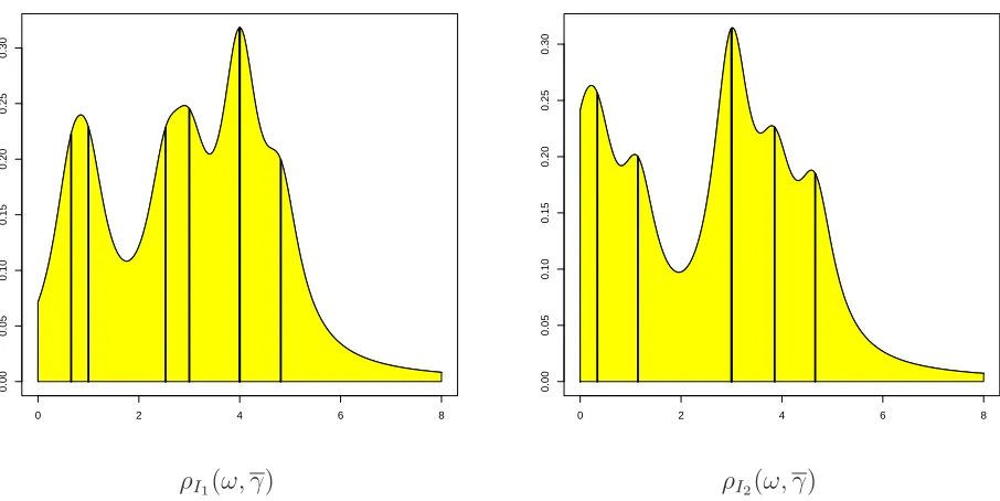
From the above spectra, we can compute the corresponding Cauchy-Lorentz
distributions ρI{1,2}(ω, γ), where γ = 0.4450034: their plots are shown in
2.2. BIOLOGICAL NETWORKS CHAPTER 2. BACKGROUND AND NOTATION
AI2 =
0 1 0 0 0 1 1 0 1 0 0 0 1 1 0 0 0 0 0 0 0 0 0 0 0 0 0 0 0 0 1 1 0 1 0 0 0 0 0 0 1 1 0 0 0 0 0 0 1 0 0 1 0 0 0 1 0 0 0 1 0 0 1 0
0 1 2 3 4 5 6 7
Figure 2.4: Adjacency matrix and graphical representation of I2
2.2
Biological Networks
Citing Barabasi in [16], “We will never understand the workings of a cell
if we ignore the intricate networks through which its proteins and metabo-lites interact with each other”. In fact, all elements of a cell, from the genes in the DNA to the molecules involved in the signal transduction mecha-nisms, are deeply interconnected at various levels: all these elements and their connections are described by all the structures known as biological networks. The need for adopting a novel approach to mine the underlying knowledge is nowadays shared by the entire community of researches, as well as the need for a common new language to benefit from contributions
from different disciplines [90].
For an exhaustive description of the biological networks, we refer to [158,
0 2 4 6 8
0.00
0.05
0.10
0.15
0.20
0.25
0.30
0 2 4 6 8
0.00
0.05
0.10
0.15
0.20
0.25
0.30
ρI1(ω, γ) ρI2(ω, γ)
Figure 2.5: Lorentzian distribution of the Laplacian spectra for I1 and I2. Vertical lines indicate eigenvalues.
153, 27]; hereafter we recall some basic facts and properties.
Networks in biology can be grouped under a few major categories:
• Gene Regulatory (or Transcriptional) Network: it is the structure
representing the mutual interactions (RNA and protein expression products) within a cell of a collection of DNA segments through their RNA and protein expression products), thus regulating the rates at which genes in the network are transcribed into mRNA. Some of the interacting factors serve only to activate other genes, and they are called the transcription factors.
• Proteinprotein interaction network: it is the structure (called
inter-actome) collecting all the binding occurring between proteins in a organism.
2.2. BIOLOGICAL NETWORKS CHAPTER 2. BACKGROUND AND NOTATION
by phosphorylation.
• Metabolic interaction network (or metabolic pathway): includes the
chemical reactions of metabolism and the regulatory interactions that guide these reactions, thus collecting all metabolic and physical pro-cesses that determine the physiological and biochemical properties of a cell.
• Signalling network: it is the network of reactions that govern how
a cell responds to its environment, together with the corresponding
dynamic flow through the network (transduction) (e.g, from a receptor
to a transcription factor that modifies expression of a gene).
A graphical display of the five above categories is shown in Fig. 2.2,
origi-nally included in [158].
Although the above networks are very diverse and heterogeneous, they all share a few key characteristics. One of the most powerful empirical rules derived by biological observations is that their topology is sparse: there is a small constant number of edges per node, much smaller than the total number of nodes. For instance, genes are regulated by a constant number of other genes (2-4 in bacteria, 5-10 in eukaryotes). Recent studies have shown that the frequency distribution of connectivity of nodes in biologi-cal networks tends to be long tailed, similar to a power-law distribution. Thus, biological networks are modeled according to a scale-free
distribu-tion: P(k) = k−γ , where k is the degree (number of connections) and
γ is some network-specific constant. The scale-free nature of gene
net-works yields the emergence of hubs (highly connected nodes) which are central in the network and are responsible for a large amount of over-all regulation. Thus, the rest of the nodes are connected by very short paths, yielding overall short longest-path between nodes. This handful of highly connected nodes also support network integrity, making networks
20 CHAPTER 2. BACKGROUND AND NOTATION
robust against random failures but exceedingly vulnerable upon targeted attack. Biological networks are very robust to fluctuations of their param-eter values and there are strong indications that only specific topologies can guarantee such robustness. In fact, the resistance to noise is one of the main effects of the intrinsic robustness of networks to random fluctuations (for instance, of the concentration of regulators) and it is an important fea-ture also when considering the modelling process. This is a fundamental characteristic as the input to the modelling process are observations of a bi-ological phenomenon that are typically very noisy. As observed by Wuchty
and colleagues in [153] all these properties are biologically grounded by
the fact that many mutations have little or no phenotypic effect, which is coherent with the occurrence of genes that either cannot propagate their failure or whose function can be taken care of by different part is of the network. On the other hand, the presence of genes supporting multiple signaling and thus responsible for widespread changes upon their failure proves the crucial role of hubs.
2.3
Network Inference
As observed by Hurley and coworkers in [64], in the last five years the
num-ber of published algorithms for reconstructing a biological network from high-throughput measurements has grown exponentially, and they have helped unveiling significant biological findings in several species, from sim-ple organisms to humans. The nature of the proposed algorithms is very heterogeneous, ranging from algebra, to differential equations to
probabil-ity: see for instance [40, 102, 111] for some comparative reviews. However,
no single method has emerged as the best performing across a wide range of tasks, as shown for instance by the outcome of the various editions of
2.3. NETWORK INFERENCE CHAPTER 2. BACKGROUND AND NOTATION
conclusion drawn from in the last edition is that, in average, the integra-tion of results coming from different methods can be an effective strategy
[99].
In this thesis, we will mainly deal with two kinds of methods: the former aims at detecting interactions as nodes’ coexpression, while the latter tries
to spot also indirect dipendencies. As described in [102] and proved on a
wide range of situations in [3], coexpression networks are biologically sound
structures in describing complex interactions. They are constructed by computing a similarity score for each pair of genes (as weighted networks), or reduced to unweighted graphs after thresholding the similarity above a certain value. The underlying rationale, called the guilt-by-association heuristic, is the assumption that if two genes show similar expression
pro-files, they are supposed to follow the same regulatory regime, i.e.,
coexpres-sion is a reasonable approximation of coregulation. The Weighted Gene Coexpression Network Analysis (WGCNA) and the Topological Overlap Matrix (TOM) approaches described hereafter follow this line, and
differ-ent correlation measure can be used within its framework (see Sec. 2.3.1).
However, coexpression networks cannot distinguish direct from indirect dependencies based on the similarity of expression patterns: for
exam-ple, a graph of three nodes X, Y, Z mutually connected by coexpression
can match different regulatory schemes X → Y → Z, X → (Y, Z) or
even W →(X, Y, Z) for an external node W. To deal with this issue other methods have been developed: among these, Algorithm for the Reconstruc-tion of Accurate Cellular Networks (ARACNE) and Context Likelihood of Relatedness are probably the most widely used by researchers worldwide. We provide in the following section a brief description of ARACNE and CLR, together with the description of a novel method called Reverse En-gineering Gene Networks by Artificial Neural Networks (RegnANN) aimed at detecting indirect interactions with higher stability.
(a) (b)
Figure 2.7: Adjacency functions for different parameter values. a) Sidgmoid and signum adjacency functions. b) Power and signum adjacency functions. The value of the adja-cency function (y-axis) is plotted as a function of the similarity (co-expression measure). Note that the adjacency function maps the interval [0,1] into [0,1]. [61, 154]
2.3.1 Weighted Gene Coexpression Network Analysis
WGCNA [154, 88] is a general framework for “soft” thresholding that
weights each connection by a number in [0,1]. In gene coexpression
net-works, each gene corresponds to a node. With the aim of retrieving the adjacency matrix of the network starting from the data, one needs first to define a measure of similarity between the expression profile of two genes.
In general the similarity measure s quantifies the level of connection
be-tween the two measured gene profiles. Applying s to any possible couple
(i, j) of genes in the dataset we obtain the n ×n matrix S = [sij]. The
next step is to transform the S matrix into an adjacency matrix A = [aij]
2.3. NETWORK INFERENCE CHAPTER 2. BACKGROUND AND NOTATION
In the WGCNA pipeline at this point the resulting adjacency matrix is used to define a measure of node distance used to define network modules through a clustering phase. At this point various intramodular and inter-modular features can be computed such as for example the intrainter-modular
connectivity that helps determine the significance of a module [61].
In this thesis we chose to use as function sthe absolute value of the Pearson
correlation sij = |cor(i, j)| or the Maximal Information Coefficient measure
(MIC). The only constraint for the similarity measure is that to be bounded
in [0,1]. The adjacency function is a monotonically increasing function that
maps the interval [0,1] into [0,1]. We can divide the adjacency functions
into two main families: soft thresholding and hard thresholding functions; as the names suggest the former functions produce weighted adjacency matrices while the second ones produce (binary) unweighted adjacency matrices. The most widely used adjacency function is the signum function that applies a hard threshold to the similarity values. The application of
this function implies the very delicate choice of the parameter τ so that:
aij = sign(aij, τ) ≡
1 if sij ≥τ
0 if sij < τ
It is obvious that an erroneous choice of the parameter τ can lead to a
loss of information, since, for instance setting τ = 0.7 means that a value
of cor = 0.69 would lead to no link at all in the final adjacency matrix.
To avoid hard thresholding, in [154] two soft thresholding methods are
proposed: the sigmoid function
aij = sigmoid(sij, α, τ0) ≡
1
1 +e−α(aij−τ0) ,
with parameters τ0 and α and the power adjacency function
aij = power(sij, β) ≡ |sij|β ,
with the only parameter β. For the experiments in this thesis we decided
to use the power adjacency function since the parameter β can be chosen
to approximate the sigmoid function. Another advantage of the use of the
power function is that if sij factors so that sij = sisj then aij factors as
well, aij = aiaj with ai = (si)β. In [154] is shown that the two adjacency
functions produce very similar results provided that the parameters are chosen following the scale-free topology criterion. The most critical step in
this approach is the choice of the parameterτ or β depending on the choice
of the functions. The choice of the parameters determines the sensitivity
and specificity of the pairwise connection strengths. For example if τ is
set too low we could incur in too many false positive links in the matrix
reconstruction because of the effect of noisy data. On the other hand, if τ
is set to high we will have an adjacency matrix too sparse, and thus we lose important information about the structure of the connections. In order to solve this problem several approaches have been applied in the literature to threshold the significance level of the correlation instead of the correlation coefficient itself. The significance level of a correlation coefficient can be estimated by using the Fisher transformation. Thus thresholding a cor-relation coefficient is replaced by thresholding the corresponding p-value. Finally, instead of focusing on the significance of the correlation or the network size, we propose to pick the threshold by making use of the fact that despite significant variation in their individual constituents and path-ways, metabolic networks have been found to display approximate scale
free topology [70, 119, 61].
2.3.2 Topological Overlap Matrix
partic-2.3. NETWORK INFERENCE CHAPTER 2. BACKGROUND AND NOTATION
ular the Topological Overlap of the couple of nodes (i, j) is:
ωi,j =
lij +aij
min{ki, kj}+ 1−aij
where lij = Puaiuauj and ki = Puaiu is the node connectivity. In case of
hard thresholding we have that lij equals the number of common neighbors
of the nodes i, j that are connected. The Topological Overlap ω(i, j) equals
one if the node with lower connectivity is connected with a set of nodes that
are also neighbors of the other node and i and j are directly connected. On
the other hand we have that ω(i, j) is zero in case that i and j are
discon-nected and they share no neighbors. The formula of TOM is generalizable
to weighted adjacency matrices just using the weighted 0 ≤ aij ≤ 1 in
the formula above. Moreover since lij ≤ min(Pu6=j aiu,Pu6=iaju) it follows
that lij ≤ min(kikj) −aij therefore if 0 ≤ aij ≤ 1 then 0 ≤ lij ≤ 1. The
topological overlap matrix Ω = [ωij] is a similarity measure [78] since it is
non-negative and symmetric [154].
2.3.3 Aracne
Aracne is a method originally written to cope with the complexity typical of the regulatory networks of the mammalian cells. It is anyways able to address more general deconvolution problems such as transcriptional and metabolic networks. This technique has been designed especially to avoid the problem of false positive which affects the great part of algorithms based on co-expression. Applying the Data Processing Inequality (DPI),
Aracne can remove the majority of indirect links [101, 109, 35]. In this
thesis we used the algorithm implementation provided on Bioconductor
[104] and the default tolerance values for DPI were used. As often
hap-pens, Aracne makes use of a hard thresholding for the binarization of the resulting adjacency matrix. As many other methods, ARACNE relies on the definition of a threshold for the binarization of the adjacency matrix.
In absence of a good heuristic for defining such threshold, on the synthetic data-sets we will adopt the area under the curve (AUC) as performance metric.
2.3.4 CLR
CLR is based on the mutual information score and can be seen as an
evolution of the class of the relevance network algorithms [46] designed to
predict the relations between transcription factors and target genes. The evolution of CLR stands in an additional step of background correction added to the phase of mutual information estimation. At first for each gene a statistical likelihood of the mutual information score is computed with respect to its network contest. Then for each couple Transcription Factor-Target Gene, the mutual information score is compared to the context
likelihood of both the elements and turned into a z-score. In this thesis we
used the implementation presented in [104]. As in the case of ARACNE,
in absence of a good heuristic for defining a binarization threshold for the inference of the adjacency matrix, on the synthetic data-sets we will adopt the area under the curve (AUC) as performance metric.
2.3.5 RegnANN
RegnANN [56] reconstructs networks through an ensemble of feed-forward
multilayer perceptrons. Each member of the ensemble is essentially a multi-variable regressor (one to many) trained using an input expression matrix to learn the relationships (correlations) among a target gene and all the other genes. Formally, let us consider the multilayer perceptron as in Fig:
2.8 (right):1 input neuron I, 1 layer of H hidden units and 1 layer of K
output units. Indicating with g the activation function of each unit and
2.3. NETWORK INFERENCE CHAPTER 2. BACKGROUND AND NOTATION
Figure 2.8: The ad hoc procedure proposed to build the training input/output patterns starting from a gene expression matrix.Each input pattern corresponds to the expression value for the selected gene of interest.
the hidden layer and with ˆwh the weights of the links between input neuron
and hidden layer, the value Ok for the output unit k can be calculated as
follows:
Ok = g H
X
h=1
wh,k·g( ˆwh·I)
!
The value Okis the inferred interaction between the corresponding gene
k and the gene associated with the input neuron I. We proceed in
de-termining the interactions among genes separately and then we join the information to form the overall gene network. From each row of the gene expression matrix we build a set of input and output patterns used to
train with back-propagation [22] a selected multilayer perceptron. Each
input pattern corresponds to the expression value for the selected gene of interest. The output pattern is the row-vector of expression values for all the other genes for the given row in the gene expression matrix (Figure
2.8). By cycling through all the rows in the matrix, each regressor in the
ensemble is trained to learn the correlations among one gene and all the others. Repeating the same procedure for all the columns in the expres-sion matrix, the ensemble of multi-variable regressors is trained to learn the correlations among all the genes. The procedure of learning separately
the interactions among genes is very similar to the one presented in [127],
where the authors propose to estimate the neighborhood of each gene (the correlations among one gene and all the others) independently and then joining these neighborhoods to form the overall network, thus reducing the problem to a set of identical atomic optimizations.
We build N (one for each of the N genes in the network) multilayer
per-ceptrons with one input node, one layer of hidden nodes and one layer of
N−1 output nodes, adopting the hyperbolic tangent as activation function.
The input node takes the expression value of the selected gene rescaled in
[−1,1]. The number of hidden nodes is set to the square root of the number
of inputs by the number of outputs. This value is to be considered a rule of thumb granting enough hidden units to solve the regression problem and allowing dynamical adaptation of the structure of RegnANN to the size of the biological network under study. The output layer provides continuous
output values in the range [−1,1].
The algorithm of choice for training each multi-layer perceptron is the
back-propagation algorithm [22]. The back-propagation is a standard algorithm
2.3. NETWORK INFERENCE CHAPTER 2. BACKGROUND AND NOTATION
The back-propagation algorithm starts with the forward-propagation of the input value in the multilayer perceptron, followed by the backward propagation of the errors from the output layer toward the input neuron. The algorithm corrects the weight values according to the amount of error each unit is responsible for. Formally, the weight values at learning epoch
τ are updated as follows:
∆w(τ) = −η∇E +µ∆w(τ−1)
To keep the notation simple w refers to both the weights associated with
the links between the output layers and the hidden layer and with the
weights of the links between input neuron and hidden layer. ∇E refers to
the gradient of the error in weight space. η is the learning rate;µ is the
momentum.
Although back-propagation is essentially a heuristic optimization method
and alternatives such as Bayesian neural network learning [108] have more
sound theoretical basis, in the proposed multi-variable regression schema the simple back-propagation algorithm allows us to design a far less com-plex system. This is due to how Bayesian neural network learning handles
the regression problem. As indicated in [107]: Networks are normally used
to define models for the conditional distribution of a set of target values given a set of input values.[...]. For regression and logistic regression mod-els, the number of target values is equal to the number of network outputs. This implies that in the case of Bayesian learning an extra procedure is required to discretize the target values from the continuous range [-1,1] and
that for each ensemble member the layer of output neurons (N −1 in the
case of back-propagation) has to be translated into a matrix of neurons of
size (N −1)×T, where T is the number of desired target values.
Accord-ingly, also the hidden layer becomes a matrix of neurons, each one with its own set of parameters. Thus, in the context of multivariable regression,
adopting back-propagation allows us to design a lower complexity inference system limiting issues related to high dimensional settings. Once the en-semble is trained, the topology of the gene regulatory network is obtained by applying a second procedure. Considering each gene in the network separately, we pass a value of 1 to the input neuron of the correspondent multilayer perceptron, consequently recording its output values. The con-tinuous output values in the range [-1,1] represent the expected normalized expression values for the other genes (its neighborhood). This procedure basically aims at verifying the correlation between the input gene and all the others: assuming the input gene maximally expressed (the value 1), an output value of 1 indicates that the correspondent gene will be also maxi-mally expressed, thus indicating perfect correlation between the two genes. An output value of -1 indicates that the correspondent gene will be max-imally under-expressed: perfect anti-correlation of the two genes. Thus, the continuous output values in the range [-1,1] are interpretable in terms
of positive correlation (> 0), anti-correlation (< 0) and no-correlation (0).
By cycling this procedure through all the ensemble members in the
regres-sion system, we obtain N (one for each of the N genes in the network)
vectors of length N − 1 of continuous values in [-1,1]. The correlation
matrix is obtained by correctly joining the N vectors. It is important to
2.4. CORRELATION MEASURES CHAPTER 2. BACKGROUND AND NOTATION
2.4
Correlation Measures
2.4.1 Pearson
In statistics the Pearson correlation index between two variables is a mea-sure of the linearity between the variables and it is computed as the ratio of their covariance and the product of the respective standard deviations.
Given two variables x and y their Pearson correlation is thus defined as
follows:
ρxy =
σx,y
σxσy
whereσxy is the covariance of the variables whileσxandσy the two standard
deviations. The value of ρxy ranges in [−1,1]: when ρxy is greater than 0
the two variables are said to be directly correlated, if ρxy is smaller than 0
then x and y are inversely correlated. If ρxy equals 0 then the variables are
uncorrelated. Pearson indexes of n variables can be collected in a squared
matrix of dimension [n×n] which will be symmetric and with the diagonal
equal to 1 since ρij = ρji and ρii = σσii2
i .
2.4.2 Biweight Midcorrelation
In order to overcome the problem of outlaiers in Pearson correlation in [152]
is proposed the bicorrelation which is considered to be a good alternative
to the standard correlation. Such algorithm was also applied in [128] by
Song and coworkers proving that, using as reference the gene ontology enrichment, the bicorrelation coupled with TOM performs better than a MIC based approach in the detecting of submodules.
To define the biweight midcorrelation of two variables x = (x1, . . . , xm)
and y = (y1, . . . , ym) we first define ua and ub with i = 1, . . . , m:
ua =
xa −med(x)
9mad(x) ub =
yb −med(y)
9mad(y) (2.1)
wheremed(x) stands for the median ofxandmad(x) is the median absolute
deviation of x this allow us to define the weight wa of xa as: