Integrated Engineering Development Environment »

The Mathematica® Journal

Integrated Engineering

Development

Environment

Oliver Rübenkönig

Zhenyu Liu

Jan G. Korvink

The IMTEK Mathematica Supplement (IMS) provides the basis for an Inte-grated Engineering Development Environment (IEDE). In this context we created an open source linear finite element modeling environment com-prising the mechanics, fluidics, and a general differential operators domain. We split the operators from the geometry and shape functions, resulting in symbolic operators, which are well suited for finite element code generation, and fast numerical operators. In this article we show how we use the fast numerical operators for analyzing a microelectromechani-cal system device. A fast transient solution by means of model order reduc-tion is presented. Finally, we conclude with a harmonic analysis.

‡

Introduction

The IMTEK Mathematica Supplement (IMS) is a downloadable open source add-on package for Mathematica [1]. The supplement provides several hundred functions in about 40 packages. At IMTEK (the Institut für Mikrosystemtechnik) we encounter a variety of engineering tasks. The tasks range from modeling to analysis and culminate in the ultimate engineering goal—good design.

Unfortunately, the design process is often tedious for several reasons. It may be very difficult to extend existing Integrated Engineering Development Environ-ments (IEDEs) due to their being closed source. Exporting some parts of the design process to controllable external tools and applying new algorithms is time-consuming. We try to remedy this shortcoming by providing the open source basis for an IEDE embedded in Mathematica.

‡

Integrated Engineering Development Environment

An IEDE consists of several pieces that can be smoothly interchanged to reach a design. The ability to model and simulate several different physical domains (e.g., the electrical engineering and mechanical domains) must be combined with the ability to analyze.

This can be accomplished with an adequate data structure, which must be applicable to other—not yet conceived—domains. We will demonstrate this process with a Finite Element Method (FEM) analysis example and later show how this concept is extendable. The finite element code is based on [2, 3, 4].

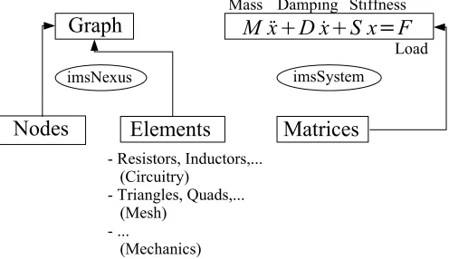
We start from the observation that engineering systems are constructed by some “basic” components that are related to each other via some connectivity, to be further specified. This connectivity can then be transformed into a system of ordinary differential equations (ODEs) (Figure 1).

Figure 1. Common to many engineering applications is the scenario that components are somehow connected, and, by some means, they and their representations in reality have a system of ODEs describing them.

A typical engineering application would be the components of an electrical circuit such as resistors, inductors, capacitances, and sources. These elements are connected to each other via “nodes” (Figure 2). The elements and nodes reside in a graph. The elements are not restricted to circuit elements, but can be elements such as finite elements that the engineer might need.

The system of equations is a system of second-order ODEs. The coefficients are the mass, damping, and stiffness matrices. The load is a vector of a list of multi-ple load vectors.

Figure 2. The connectivity in engineering applications can be captured with graphs consisting of nodes and elements, where the different element types come from different application areas. In IMS the data structure representing graphs is called imsNexus. The system of ODEs is represented by a system of second-order ODEs with matrix coefficients. The underlying data structures are matrices.

In this article we show how we use the graph data structure, apply finite element operators in the elements in the graph, and obtain a system of equations (Figure 3). The finite element operators are taken from the classical scalar partial differential equations (PDEs). The concept, however, is general, and for differ-ent engineering domains differdiffer-ent operators can assemble a system of equations.

In this article we show how we use the graph data structure, apply finite element operators in the elements in the graph, and obtain a system of equations (Figure 3). The finite element operators are taken from the classical scalar partial differential equations (PDEs). The concept, however, is general, and for differ-ent engineering domains differdiffer-ent operators can assemble a system of equations.

Figure 3. An operator can be applied to each of the elements in a graph. Every operator returns an element matrix (an imsElementMatrix data structure). This is then assembled into a global matrix by the assembler routine. The operators can come from a wide range of engineering areas.

‡

Heat Anemometer Application Example

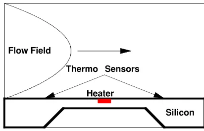
Here we model a heat flow anemometer. Figure 4 shows a schematic of the device.

Flow Field

Silicon Heater

Thermo Sensors

Figure 4. A schematic of a heat flow anemometer.

In a piece of bulk silicon we have embedded a small heater device. To the right and left are two temperature sensors. If the heater is switched on, both sensors will measure the same temperature. Once a flow field is flowing over the silicon

In a piece of bulk silicon we have embedded a small heater device. To the right and left are two temperature sensors. If the heater is switched on, both sensors will measure the same temperature. Once a flow field is flowing over the silicon device, the temperature distribution will shift and the left sensor will be cooler than the right sensor. From the temperature difference we can calculate the speed of the flow field. This is the principle of an anemometer. More about thermal measurements in fluids can be found in [5].

In the next section we calculate the temperature distribution in the device and its surrounding area.

‡

The Equation

In the most general assumption, we wish to model the following equation:

(1)

s “2_{u + g “u}

Diffusion Convection

´¨¨¨¨¨¨¨¨¨¨¨¨¨¨¨¨¨¨¨¨¨¨¨¨¨¨¨¨¨¨¨­¨¨¨¨¨¨¨¨¨¨¨¨¨¨¨¨¨¨¨¨¨¨¨¨¨¨¨¨¨Æ

= f

Load

Stiffness Matrix Load Matrix

The heater element will be modeled with a load matrix and the airflow with the convection term. The general heat transfer is modeled with the diffusion term.

‡

Loading Predefined Mesh

We begin by loading the Imtek`Interfaces`EasyMesh` package.

In[86]:= Needs"Imtek‘Interfaces‘EasyMesh‘"

Then we import the EasyMesh-generated example mesh.

In[87]:= numberOfNodes, mesherNodes, numberOfElements,

mesherElements, numberOfSides, sidesimsReadEasyMesh

ToFileName "Imtek", "IMSData", "ApplicationExamples", "FEM", "AnemometerMesh", imsStartNodeNumbering1;

·

Creating the Nodes

First we load the following packages.

In[88]:= Needs"Imtek‘Graph‘"

Needs"Imtek‘MeshElementLibrary‘"

Then we take the raw nodes and make IMS nodes from them. Each of the raw nodes is a list of a unique node identification number (id), the coordinates 8x, y<, and a marker. This marker was inserted by the mesh generator and indicates whether the node belongs to one of the domain segments or not.

We also divide the nodes into boundary nodes and interior nodes. Boundary nodes are the nodes on the simulation domain boundary that specify the bound-ary conditions. In the mesh input file we have specified that markers 1, 2, and 3 are on the simulation boundary. All other nodes are interior nodes. Either they belong to interior domain segments (and carry the marker 7) or they do not belong to any segment at all (and carry the marker 0).

The IMS nodes we create also carry a unique identification number (id), the coordinates 8x, y<, the marker, a value of the solution (initially set to 0), and the type of the boundary condition.

In[90]:= interiorNodes 

SelectmesherNodes, #4  0  #4  7& .

id_, x_, y_, marker_  imsMakeNodeid, x, y, marker;

Here we select from the list of all mesh nodes those entries where the marker is 0 or 7.

This displays all the nodes that have a marker of 7.

In[91]:= ShowGraphicsPoint#& 

# 2, 3 &  SelectmesherNodes, #4  7& , AspectRatio  0.25

The boundary nodes are those nodes that have a fourth entry not equal to 0 or 7. Additionally we set boundary conditions in the nodes according to the markers for the specific node. The nodes now carry the id, the coordinates, the marker, the boundary condition value, and the boundary condition type.

In[92]:= boundaryNodes 

SelectmesherNodes, #4  0 && #4  7& . id_, x_, y_, marker_ 

Which marker  1,

imsMakeNodeid, x, y, marker, 0., "Dirichlet", marker  2, imsMakeNodeid, x, y,

marker, 0., "Dirichlet", marker  3, imsMakeNodeid, x, y,

marker, 0., "Dirichlet" ;

·

Creating the Elements

Now we set up the elements. Dirichlet boundary conditions are only set up in the nodes. Neumann boundary conditions also need an entry in the elements. Each element consisting of two Neumann boundary nodes will additionally carry the boundary values for the nodes involved.

First we join all nodes and obtain the Neumann boundary node ids.

In[93]:= allNodes  SortJoininteriorNodes, boundaryNodes, OrderedQ imsGetIds#1, imsGetIds#2  &; neumannBoundaryNodesIds  imsGetIds

SelectboundaryNodes, imsGetDatas# "Neumann" & 

Out[94]= 

To construct the elements, we choose those elements that have a count of two Neumann boundary nodes and insert the Neumann values of the boundary nodes into the elements. All other elements are constructed in such a way that they carry their identification id, the incident ids (i.e., the ids of the nodes making up the specific element), and the element marker.

The element marker, in contrast to the node marker, states to which of the four parts of the simulation device the element belongs. Marker 1 is for the silicon device, marker 2 is the heater, marker 3 is the free cut, and marker 4 is the flow box.

In[95]:= allElements 

mesherElements . id_, i_, j_, k_, ei_, ej_, ek_, si_, sj_, sk_, xV_, yV_, marker_ 

IfPlus  CountneumannBoundaryNodesIds, #& 

i, j, k   2,

imsMakeTriangleLinear1DOFid, i, j, k, marker, imsGetValuesallNodes i, j, k   ,

imsMakeTriangleLinear1DOFid, i, j, k, marker ;

Each element has a marker similar to the markers in a node. The element markers can later be used to specify the behavior of finite element functions in different areas of the mesh.

·

Creating the Mesh

Now we generate the mesh.

In[96]:= femMesh  imsMakeNexusboundaryNodes, interiorNodes, allElements;

In[97]:= numberOfNodes

Out[97]= 3991

In[98]:= numberOfElements

Out[98]= 7785

Since each node belongs to several triangles, we have more triangles than nodes.

·

Displaying the Mesh

Here we display the mesh.

In[99]:= ShowGraphics imsDrawElementsfemMesh, device , PlotRange  All, AspectRatio  Automatic

Here we display the mesh inside the silicon and those elements with marker 1.

In[100]:= siliconElementIds  imsGetIds

SelectimsGetElementsfemMesh, imsGetMarkers#  1& ;

In[101]:= ShowGraphics imsDrawElementsfemMesh, siliconElementIds  , PlotRange  All, AspectRatio  0.25

‡

Physics Setup

The finite element operator functions need some further specifications. For example, the diffusion operators need some information about the isotropy of the material underneath, and each finite element operator needs a function to specify its behavior. Setting the function values to 0 will turn off the operator in that region. The functions obtain the marker of the element they are currently computing and the coordinates of the center of mass of this element. This information should be enough to specify complex functions in complex regions.

We have not spoken about the dimensions of the device. For meshing it was convenient to set the dimensions to 10-6 (i.e., a micrometer scale). That implies, however, that we have to scale the material data accordingly. This is what the xyScale values do.

We have four markers for the elements. Depending on where an element is physically situated in the simulation domain, it may have different properties. We have four parts in our simulation domain. The silicon parts (silicon device and heater) have different material data than the air parts (free cut and flow box). The convection part of the equation is only active in the flow box part of the simulation domain. Thus, in the other parts we set the convection function to 0. The heater is similar. With this mechanism we can switch different parts of the PDE on and off in different parts of the simulation domain.

·

Anisotropy

We assume the heat conduction of silicon to be 148 W/(K m) and that of air to be 23.9*10-3 W/(K m).

In[102]:= anisotropyScale  10^6;

anisotropyFunction  Function marker, x, y, Evaluate

Which marker  1,

EvaluateanisotropyScale148.  1., 0., 0., 1.  , marker  2, EvaluateanisotropyScale

148.  1., 0., 0., 1.  ,

marker  3, EvaluateanisotropyScale23.9  10^3  1., 0., 0., 1.  ,

marker  4, EvaluateanisotropyScale23.9 

10^3  1., 0., 0., 1.   ;

·

Convection

The specific heat of air is approximately 1000 J/(Kg K) and the density is 1.29 Kgêm3_.

In[104]:= convectionScale  1.; velocity  10 ^1.;

convectionFunction  Function marker, x, y, Evaluate

Which

marker  1, 0., 0., marker  2, 0., 0., marker  3, 0., 0., marker  4,

EvaluateconvectionScale  10001.29 velocity   yanemometerHeight  flowHeight2  

flowHeight2 ^2 1, 0.  ;

·

Load

We have a heat source of 1010 Kgê Hs2_mL_.

In[107]:= loadScale  10^6;

loadFunction  Function marker, x, y, Evaluate

Which

marker  1, 0.,

marker  2, EvaluateloadScale10 ^10., marker  3, 0.,

marker  4, 0. ;

In[109]:= Graphics‘PlotField‘

In[110]:= PlotVectorFieldFlattenconvectionFunction4, x, y ,

x, baseX, anemometerLength,y, anemometerHeight, anemometerHeight  flowHeight, PlotRange  All

‡

Steady-State Solution

·

Initialization

First we load the Imtek`ShowStatus` package.

In[111]:= Needs"Imtek‘ShowStatus‘"

·

Matrix Assembly

In[112]:= Needs"Imtek‘FEMOperators‘" Needs"Imtek‘Assembler‘"

The assembly of the global matrix is divided into several steps. First we need to initialize the required global matrices, the stiffness matrix, and the load vector. The element dimension specifies the size of the element stiffness matrix and the element right-hand side vector. We want to loop over all elements. First we get the element (let us call it i) from the mesh and get this element’s nodes. We also need the rows and columns that this element contributes to in the global matrix.

First we create two matrices with 0 entries—one for initializing each element stiffness matrix (elementSMEmpty) and one for initializing the element right-hand side (elementRHSEmpty).

In the main computation each operator is applied to each element i. The input to each operator is an element matrix and an element right-hand side matrix. Each operator also returns those two matrices, now occupied by the values computed for this element. The order in which the operators are applied does not matter. In the last step the element matrix is assembled into the global matrix.

In[114]:= stiffness  SparseArray ,numberOfNodes, numberOfNodes, 0.; load  Table0., numberOfNodes, 1 ;

In[116]:= elementDim 

LengthimsGetIncidentsIdsimsGetElementsfemMesh, 1  ;

In[117]:= elementSMEmpty  Table0.,elementDim,elementDim; elementRHSEmpty  Table0.,elementDim,1;

In[119]:= Do

imsShowStatus"Computing Element Number: "

ToStringi  " from "  ToStringnumberOfElements ;

element initialization

thisElement  imsGetElementsfemMesh, i; elementNodes 

imsGetNodesfemMesh, imsGetIncidentsIdsthisElement ; rows  cols  imsGetIdselementNodes;

elementSM  imsMakeElementMatrixelementSMEmpty, rows, cols; elementRHS  imsMakeElementMatrixelementRHSEmpty, rows, 1 ;

main computation elementSM, elementRHS 

imsNFEMDiffusion elementSM, elementRHS, thisElement, elementNodes, anisotropyFunction;

elementSM, elementRHS 

imsNFEMLoad elementSM, elementRHS, thisElement, elementNodes, loadFunction;

elementSM, elementRHS 

imsNFEMConvection elementSM, elementRHS, thisElement, elementNodes, convectionFunction;

elementSM, elementRHS 

imsNFEMNeumann

elementSM, elementRHS, thisElement, elementNodes;

build the global stiffness and load imsAssembleelementSM, stiffness; imsAssembleelementRHS, load;

,i, numberOfElements ;

·

Dirichlet Boundary Conditions

The last step before solving the system of equations is to build in the Dirichlet boundary values. For this we load the Imtek`BoundaryConditions` package.

In[120]:= Needs"Imtek‘BoundaryConditions‘"

Then we select the Dirichlet boundary nodes from the mesh.

In[121]:= diriNodes  SelectimsGetBoundaryNodesfemMesh, imsGetDatas#  "Dirichlet" &;

The Dirichlet operators get a matrix (stiffness), a vector (flattLoad), and the position and value of the Dirichlet boundary condition. We create a list of position (node id) and value pairs.

In[122]:= positionValuePairs  Transpose

imsGetIdsdiriNodes, FlattenimsGetValuesdiriNodes, 1   ;

This maps the Dirichlet operator on the list of position and value pairs.

In[123]:= flattLoad  Flattenload;

MapimsDirichlet stiffness, flattLoad, #1, #2 &, positionValuePairs;

·

Solving

In[125]:= Needs"Imtek‘System‘"

In[126]:= load  PartitionflattLoad, 1;

stationarySystem  imsMakeSystemload, stiffness 

Out[127]= imsSystem3991,1, 1, 0, 0

To solve the system of equations we load the Imtek`SystemAnalysis` package.

In[128]:= Needs"Imtek‘SystemAnalysis‘"

In[129]:= solution  imsStationarySolvestationarySystem;

·

Initialize Post Process

Now we look at the result.

First we set the values of the solution into the nodes. Since a node may contain solution values at several time steps—which we so far do not have—we partition the solution into sublists of size 1 (see Nodes in the IMTEK documentation in the Help Browser).

In[130]:= newNodes  imsSetValuesallNodes, Partitionsolution, 1 ;

We then sort them into boundary and interior nodes.

In[131]:= newBoundaryNodes 

newNodesimsGetIdsimsGetBoundaryNodesfemMesh  ; newInteriorNodes 

newNodesimsGetIdsimsGetInteriorNodesfemMesh  ;

Here we create a new graph with the new nodes that carry the solution.

In[133]:= solutionMesh 

imsMakeNexusnewBoundaryNodes, newInteriorNodes, allElements;

·

Contour Plot

To visualize a contour plot of the solution, we sort the nodes and obtain their coordinates.

In[134]:= coordinates  imsGetCoordsSortimsGetNodessolutionMesh, OrderedQimsGetIds #1, #2  & ;

Next we obtain the incidents.

In[135]:= incidents  imsGetIncidentsIdsimsGetElementssolutionMesh ;

Then we load the Imtek`UnstructuredPlot` package.

In[136]:= Needs"Imtek‘UnstructuredPlot‘"

To set the contours we find the minimum and maximum values.

In[137]:= minSol, maxSol  Minsolution, Maxsolution

Out[137]= 0., 0.119914

In[138]:= stepSize  maxSol minSol 30.

Out[138]= 0.00399714

Here is the result.

In[139]:= femP 

imsUnstructuredContourPlotcoordinatesRangenumberOfNodes , incidents, Flattensolution, AspectRatioAutomatic,

ContoursRangeminSol, maxSol, stepSize, MeshFalse, PlotRange  All, DisplayFunction  Identity;

In[140]:= Show femP, Graphicsdevice , DisplayFunction  $DisplayFunction

‡

Transient Solution via Model Order Reduction

·

The Equation

Now we model the following equation:

(2)

r ÅÅÅÅÅÅÅÅÅÅ∂u ∂t Transient

+ s “2_{u + g “u}

Diffusion Convection

´¨¨¨¨¨¨¨¨¨¨¨¨¨¨¨¨¨¨¨¨¨¨¨¨¨¨¨¨¨¨¨­¨¨¨¨¨¨¨¨¨¨¨¨¨¨¨¨¨¨¨¨¨¨¨¨¨¨¨¨¨Æ

= f

Load

Damping Matrix Stiffness Matrix Load Matrix

The new term is the partial time derivative.

·

The Physics

In order to scale the damping function correctly, we need to set the damping function. With the specific heat of approximately 700 J/(Kg K) for silicon and 1000 J(Kg JK) for air. The densities are 2330 Kgêm3 _{for silicon and 1.29 Kg}ê_m3

for air.

In[141]:= dampingScale  10^6.;

In[142]:= dampingFunction  Compile  marker, _Integer, x, y, EvaluateWhich

marker  1, EvaluatedampingScale7002330, marker  2, EvaluatedampingScale7002330, marker  3, EvaluatedampingScale1000.1.29, marker  4, EvaluatedampingScale1000.1.29 ;

·

The Damping Matrix Assembly

Since the stiffness matrix has already been assembled, we now devote our atten-tion to the damping matrix matC. This approach is exactly the same as for the stiffness matrix. Now, however, we use the FEMTransient operator.

First we create an empty sparse array for the damping matrix.

In[143]:= damping  SparseArray ,numberOfNodes, numberOfNodes, 0.;

Next we obtain the element dimension and create an empty element damping matrix and an empty right-hand side matrix.

In[144]:= elementDim 

LengthimsGetIncidentsIdsimsGetElementsfemMesh, 1  ;

In[145]:= elementDMEmpty  Table0.,elementDim,elementDim; elementRHSEmpty  Table0.,elementDim,1;

While assembling the stiffness matrix, we used a Do loop. Now we look at a more functional programming style. First we get all elements for the mesh.

In[147]:= allElements  imsGetElementsfemMesh;

Next we obtain all element nodes, element rows, and columns.

In[148]:= allElementNodes 

imsGetNodesfemMesh, #&  imsGetIncidentsIdsallElements; allRows  allCols  imsGetIdsallElementNodes;

We create all empty element matrices with the correct row and column entries.

In[150]:= allEmptyElements  

imsMakeElementMatrixelementDMEmpty, #, #,

imsMakeElementMatrixelementRHSEmpty, #, 1 & allRows;

Now we thread the transient operator over all empty elements.

In[151]:= allFilledElements 

ThreadimsNFEMTransientMatrixallEmptyElements, allElements, allElementNodes, dampingFunction ;

In the last step we assemble the filled local damping and right-hand side matrices into the global damping matrix and the global right-hand side vector.

In[152]:= Map

imsAssemble#1, damping;

imsAssemble#2, load;&, allFilledElements;

To account for the Dirichlet values, we set the matrix entries to 0.

In[153]:= dampingAll, positionValuePairsAll, 1   dampingpositionValuePairsAll, 1, All 0.;

Finally, we generate a transient system.

In[154]:= transientSystem  imsSetDampingstationarySystem, damping 

Out[154]= imsSystem3991,1, 1, 1, 0

·

Model Order Reduction

To perform a transient simulation, it is useful to reduce the order of the equation system and to thus accomplish the transient solution in a short time.

First we load the Imtek`Arnoldi` package.

In[155]:= Needs"Imtek‘Arnoldi‘"

Then we reduce our original system to the dimension we want.

In[156]:= dimension  30;

reducedSystem, matV 

imsArnoldiReductiontransientSystem, dimension;

·

Transient Solution

As an excitation we choose a unit step.

To compute the transient behavior we use TransientSolve.

In[158]:= tStart  0.; tEnd  210 ^3.

Out[159]= 0.002

In[160]:= Timing

reducedSolution 

x. imsTransientSolvereducedSystem, x, t, tStart, tEnd, UnitStep, SolveDelayedTrue, StepMonitor  imsShowStatust  

Out[160]= 0.32 Second,InterpolatingFunction0., 0.002,

Here we reverse the projection.

In[161]:= tStep  tEnd  tStart 5;

time  RangetStart, tEnd, tStep;

solutionData  TransposematV. reducedSolution#& time;

·

Post Process

The post processing is along the same lines as previously stated. This time, however, each node has several solution values, one for each time step.

In[164]:= transientNodes 

imsSetValuesallNodes, Partition#, 1&  solutionData;

In[165]:= boundaryNodes 

transientNodesimsGetIdsimsGetBoundaryNodesfemMesh  ; interiorNodes 

transientNodesimsGetIdsimsGetInteriorNodesfemMesh  ;

Then we create a new graph with the new nodes that carry the solution.

In[167]:= solutionMesh 

imsMakeNexusboundaryNodes, interiorNodes, allElements;

·

Transient Contour Plot

The minimum of the solution value should be around zero.

In[168]:= minSol, maxSol  MinsolutionData, MaxsolutionData

Out[168]= 2.81451023, 0.116894

In[169]:= stepSize  maxSol minSol 25.

Out[169]= 0.00467578

In[170]:= ShowGraphicsArrayPartitionShow 

imsUnstructuredContourPlotcoordinates, incidents,

FlattenimsGetValuestransientNodes, Sequence#, 1  , ContoursRangeminSol, maxSol, stepSize,

PlotRange  All, AspectRatio  Automatic, DisplayFunction  Identity,

Graphicsdevice 

&  RangeLengthtime , 2 , DisplayFunction  $DisplayFunction

‡

Integrated Engineering Development Environment

Future

A future application of this example might couple the computed model with an electrical circuit model. Generally more engineering domains need to be added, which implies an implementation of new operators. The finite element operators would be extended to arbitrary dimensions and elements.

‡

Conclusion

We have shown that the concept of using graphs, operators, and system assembly can be used to create an Integrated Engineering Development Environment. Thus we have an environment in which to create different engineering domains as well as to extend and solve them. It is just a matter of plugging in new domains. We have added numerical capabilities to Mathematica in the sense that we can solve some classical PDEs on arbitrary formed domains. With model order reduction, a transient solution can be found in less time than many desig-nated commercial software tools.

‡

Acknowledgment

The authors would like to thank all the people who have contributed to IMS. The first author would like to especially thank his mentors, Professor Jan G. Korvink and Dr. Zhenyu Liu, as well as the many people who have contributed suggestions, packages, and motivation, in particular Steffen Kibbel, who made many suggestions for the anemometer example.

‡

References

[1]

[2] H. R. Schwarz, Methode der Finiten Elemente, 3rd ed., Stuttgart: B. G. Teubner, 1991.

[3] D. R. J. Owen and E. Hinton, A Simple Guide to Finite Elements, Swansea, UK: Pineridge Press, 1980.

[4] V. N. Kaliakin, Introduction to Approximate Solution Techniques, Numerical Modeling, and Finite Element Methods, New York: Marcel Dekker, 2002.

[5] H. Ernst, “High-Resolution Thermal Measurements in Fluids,” Ph.D. thesis, Albert-Ludwigs-Universität Freiburg, Freiburg, 2001.

The Mathematica Journal 10:3 © 2007 Wolfram Media, Inc.

O. Rübenkönig, Z. Liu, and J. G. Korvink, “Integrated Engineering Development Environ-ment,” The Mathematica Journal, 2012. dx.doi.org/10.3888/tmj.10.3-8.

About the Authors

Oliver Rübenkönig is a Ph.D. student at the University of Freiburg, Germany. Rübenkönig received his Diploma in Microsystem Engineering in 2001. He uses Mathematica exten-sively in research and teaching and has developed many student exercises and some courses.

Zhenyu Liu is a research assistant at the University of Freiburg, Germany. Liu received his M.S. in 1997 and his Ph.D. in 2000 from the Department of Mechanical Engineering, Dalian University of Technology in China.

Jan G. Korvink obtained his M.Sc. in computational mechanics from the University of Cape Town in 1987 and his Ph.D. in applied computer science from the ETH Zurich in 1993. After his graduate studies, Korvink joined the Physical Electronics Laboratory of the ETH Zurich, where he established and led the Modeling Group. He then moved to the Albert Ludwig University in Freiburg, Germany, where he holds a Chair position in microsystem technology and runs the Laboratory for Microsystem Simulation. Currently, Korvink is dean of the Faculty of Applied Science. He has written more than 130 journal and conference papers in the area of microsystem technology and co-edits the review journal Applied Micro and Nanosystems. His research interests include the modeling, simulation, and low-cost fabrication of microsystems.

Oliver Rübenkönig Zhenyu Liu Jan G. Korvink

Lab for Simulation, Department of Microsystems Engineering (IMTEK) University of Freiburg

Germany

[email protected]