The Black Sea Deep Current Velocities Estimated from
the Data of Argo Profiling Floats
N.V. Markova, A.V. Bagaev
Marine Hydrophysical Institute, Russian Academy of Sciences, Sevastopol, Russia e-mail: [email protected]
Considering scarce available data on the velocity field in the deep layers of the Black Sea, it is important to contribute by deriving the velocity vectors from indirect sources. The Lagrangian velocity vectors of the Black Sea currents on the depths below the main pycnocline are calculated using the data on the trajectories and actual profile depths of the Argo profiling drifters in 2005-2015. The values and directions of the calculated vectors in the layers 350 – 600, 600 – 800, 800 – 1200 and 1200 – 1600 m are analyzed. The obtained results are statistically evaluated. It is shown that the prevailing number (88%) of the modules of the calculated current velocity vectors is within the range 1 – 20 cm/s. The currents’ velocity average for the whole period of measurements, is about 4 cm/s in the layers 350 – 600 and 600 – 800 m, approximately 6 cm/s in the 800 – 1200 m layer and 3.5 cm/s in the 1200 – 1600 m layer. The mean current velocities from the whole data access are higher in January – March, whereas the lowest ones fall on June – October. On the background of general cyclonic circulation the meso-scale eddy structures on the specified depths are revealed. A discussion is presented on the available approaches to increase the precision and credibility of the obtained velocities magnitude and direction.
Keywords: the Black Sea, deepwater circulation, current velocity, Argo float.
DOI: 10.22449/1573-160X-2016-3-23-35
© 2016, N.V. Markova, A.V. Bagaev © 2016, Physical Oceanography
Introduction. Investigations on the Black Sea circulation structure and
physical mechanisms began to appear in the first half of the XX century [1, 2]. In recent years fundamental researches [e.g. 3 – 6] are supplemented with a variety of the sea upper layer dynamic studying, measuring and modeling. Indeed, the most active exchange processes, motions, and the highest temperature and salinity gradients are exactly in the upper layer.
We will list the typical thermohaline and dynamic features of the Black Sea upper layers. In the vertical structure we note the upper quasi-homogeneous layer and seasonal (spring-summer) thermocline, which are mainly related to the process of wind-induced mixing and annual cycle of heat flux over the sea surface. Then we note the cold intermediate layer waters (CIL). The CIL is the layer of minimum temperatures between the seasonal and constantpycnoclines, which is bounded by +8 °С isotherm at the depths about 50 – 100 m. Main pycnocline (the level of maximum (by depth) density gradient) waters are located below the CIL at the horizons down to ~300 m. The density is mainly determined by the salinity, and the temperature remains relatively stable. Some researchers single out the transformation zone between the CIL and deep waters as a separate (intermediate) layer. Thus, they include in this layer the main pycnocline and the underlaying waters down to 1000 – 1200 m horizons [7]. In the deep layer (horizons below 1000 – 1200 m) density value is almost constant. The processes taking place in the layer, which is deeper than 300 m will be called sub-pycnoclinic, and the circulation will be called a deepwater (sub-pycnoclinic) one.
Western parts of the sea (“Knipovich Glasses”). Quasistationary mesoscale (with the diameter of several tens kilometers) anticyclonic eddies are also one of the main features of the sea upper layer circulation. Eddies are named after the geographical objects which are located relatively close to them (e.g. Sevastopol, Batumi, Sinop anticyclones etc.) Outside the area of main gyres current velocities are lower and make up (according to various estimations) from 5 to 20 cm/s. The presence of short-lived submesoscale mainly anticyclonic eddies between the BSRC and the coast is noted.
Dynamic structure below the main pycnocline is still poorly studied. The Black Sea waters at these depths are saturated with hydrogen sulphide. Generally speaking, they are of little use for economic activities at the current stage, and this is the reason for the lack of new investigations. It is assumed that sub-pycnocline circulation direction is basically consistent with the circulation direction at higher horizons. Average over the depth current velocities decrease with the distance from the surface and by the 500 m horizon they make up about 5 – 10 cm/s. Prior to the publication of [8, 9], it was assumed that practically there were no hydrological characteristic seasonal changes in sub-pycnocline. It was also supposed that the spatial distribution of hydrological characteristic was significantly homogeneous. In [8, 9] it is revealed that the circulation varies over the time keeping its cyclonic orientation, and dynamic surface displays lots of eddies. In these papers average velocities are estimated to be about 5 cm/s. In [10] it is determined that bottom currents in some areas are caused by the bottom topography. Insufficient cover of field experiments data for the mentioned depths hinders more detailed investigations of deep currents physical nature. Summary data archive of expeditionary and float current measurements for the entire sea remains extremely small to date in spite of the increased number of stations performed in certain areas. Moreover, most of both archived and new data were obtained mainly at the horizons down to 300 – 500 m. The results of experiments based on the modern numerical models [11 – 16] allow us to reproduce three-dimensional (by the space) structure of current field for the entire basin and all over its depth. However, the experiment results still require verification with the field data at corresponding horizons. The measurements carried out by the autonomous floating buoys can be used as one of such data sources.
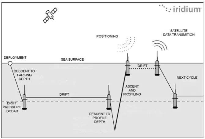
The system of autonomous deep-drifting profiling floats Argo began to develop within the framework of international project on the World Ocean monitoring in 1999 [17, 18]. In the ocean the float drifts at the specified depth. Periodically it ascents to the surface to transmit the obtained data via the satellite (Fig. 1). 27 floats were deployed into the Black Sea [17] from 2005 to 2015. For the present day 9 profiling floats are in operation. Of course, there are not as much measurement data as we would like to have for the research, but even the data array collected up to date has not been fully used for the deepwater circulation assessment.
caused by currents in the intermediate layer mostly follows the isobaths arrangement; average velocity values, which are about 5 cm/s, are given. Relatively active water circulation at the horizons corresponding to 500 – 1000 db (1 db corresponds approximately to 1 m depth) was also pointed out.
Fig. 1. An example of Argo profiling float duty cycle.
In the given paper we provide information on the calculated Lagrangian velocities of currents in the Black Sea sub-pycnocline layer at 350 – 1600 m horizons. To get it, we rely solely on the Argo drifter trajectories and maximum profiling depth data. The parking depth of 450 m, which is the closest one (from below) to the main pycnocline deep boundary, is originally taken as the upper boundary of the layer under consideration. The layer lower boundary is due to the profiling float drift maximum depth with regard to the possible deviations. Thus, measuring data of 200 m parking depth drifters (which are transporting by faster currents [1 – 8] in the main pycnocline) were not considered. The floats often drifted above their parking depth, so we could raise the upper boundary of the layer under study up to 350 m.
Similar studies are not numerous. In addition to the abovementioned papers [8, 9], the research [23] should be noted. It is based on the analysis of seven profiling float data. These floats were in operation in 2002 – 2009. In the research it was found out that mean velocities of profiling floats with 750 – 1550 m parking depths for the entire measurement period made up 2.2 – 2.7 cm/s, and the ones at 500 m parking horizon were equal to 4 cm/s. Drifter movement according their coordinates at the surface was described in details but the verification of parking depth achievement by the drifting floats was not carried out. Thus, it is not clear whether the described dynamics may be attributed to the drift horizons, or its structural elements are located in different layers vertically. This feature of Argo
Initial data and processing technique. The archives for 16 floats (which had performed the measurements in the Black Sea sub-pycnoclinic waters in 2005 – early 2015 (Table 1)) were obtained from freely accessible Argo drifter databases [20, 21]. Up to the beginning of April, 2015, more than 2000 stations were performed by such floats in total. Another 11 profiling floats were drifting in the Black Sea at that time but they were not considered in the present study, as their parking depth made up only 200 m. Downloaded data archives were additionally filtered: the information on float trajectory adequacy (i. e. on their location within the Black Sea and realistic changes of their coordinates with the time) and on the fact when the float reached the depth below 300 m was analyzed for each of 2057 profiles. In analogy with earlier papers [8, 23], drifter velocity at an appropriate depth was calculated as a ratio of distance covered to the time between the float surfacings. The data on each separately performed profile were used. It was important that the numbers of stations (performed by drifter) be placed in the archive without gaps. A loss of at least one (intermediate) station from the measurement chain results in averaging time increase and desired velocity vector determination accuracy decrease. This may occur primarily due to drifting float trajectory nonlinearity. The prevailing value of the period between profilings for the considered floats made up 120 h, average surface drift duration made up about 10 h. 10 of 16 profiling floats were positioned on the surface by the Argos satellite system, and 6 floats – by Iridium (GPS) system. In [24], the errors, introduced in the velocity calculation results due to different float positioning methods, and a communication with a satellite, as well as the ways of their elimination, are discussed.
Parking horizon selection and float duty cycle programming are carried out not by its manufacturer, but by those researchers who deploy the float in the ocean, and are determined by the researcher objectives. Most often, the drifters are placed at the horizons, which are deeper than 500 m. This is intended to make the floats forced by deep-water currents move away from the deployment area not so rapidly and to make the distance between the obtained profiles be quite short. On the contrary, in some cases it is necessary for the float to go maximum distance during its lifetime, covering with the measurements the greatest possible area of the sea. For this purpose the float is placed at a shallower depth, but this increases a risk of running ashore for it.
surrounding areas (layers). If the maximum depths of previous and subsequent measurement profiles were lesser than the parking depth but both values were located in the same layer, the calculated velocity vector was assumed to be correct and was accepted for consideration for a given layer. The layers were selected with regard for the prevailing values of parking depths: 350 – 600 m (450 and 500 m parking depths), 600 – 800 m (750 m), 800 – 1200 m (1000 m), 1200 – 1600 m (1300 and 1500 m).
T a b l e 1
The amount of calculated current velocity vectors and profiles performed in the Black Sea by the Argo floats during 2005 – 2015
Float number Operating period under consideration Positioning system Passport specifications: parking depth/maximum profiling depth, db Total number of conside red profiles The amount of calculat ed velocity vectors (in all layers) 7900465 19.06.09-20.03.12 Iridium 450/500 134 131 7900466 19.06.09-10.12.12 Iridium 450/500 187 163 6901899 15.05.14-23.11.14 Iridium 500/1000 39 35 6900803 01.04.11-14.07.13 Argos 750/1500 142 68 6900804 01.04.11-14.07.13 Argos 750/1500 166 81 6900805 31.03.11-21.03.15 Argos 750/1500 286 155 6901895 15.08.13-16.03.15 Argos 750/750 117 114 7900590 11.09.13-22.03.15 Argos 750/2000 113 69 7900593 12.07.17-28.04.15 Iridium 750/2000 60 56 7900591 29.12.13-29.04.15 Iridium 1000/1000 88 84 7900592 28.12.13-28.10.14 Iridium 1000/1000 82 55 5902291 30.04.10-16.06.10 Argos 1300/1300 24 6 4900489 27.03.05-17.08.08 Argos 1500/1550 155 121 4900540 27.03.05-15.10.08 Argos 1500/1550 173 161 4900541 14.08.06-14.03.09 Argos 1500/1550 124 122 4900542 07.08.06-05.01.10 Argos 1500/1550 161 137
The results. Four current velocity vector arrays, corresponding to each of the
modules comparable with the error of their computation. To increase the estimation accuracy it was decided to exclude such vectors from the consideration and to recalculate mean current values. The number of such small vectors made up 193 (12 % of all constructed vectors). The median of their modules is 0.8 cm/s, they are directed variously and are mostly concentrated in the western part of the sea. Small velocity values could be obtained, for example, when the float got into an eddy structure. In this case, the coordinates for the period between the surfacings changed insufficiently. The nature of such vectors needs additional analysis and investigation. So, further we will consider 88% of all calculated vectors and 66 % of all profiles measured by floats.
Fig. 2. Current velocity vectors: а –in 350 – 800 m layer (450, 500, 750 m parking depths); b –in 800 – 1600 m layer (1000, 1300, 1500 m parking depths)
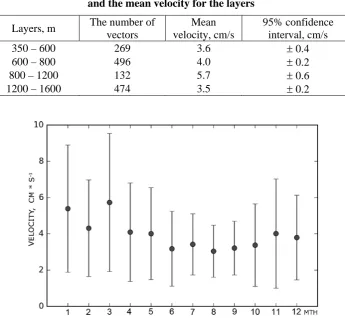
The mean velocity in 350 – 600 m and 600 – 800 m layers is approximately the same and it makes ~4 cm/s; in 800 – 1200 m layer it makes approximately 6 cm/s, in 1200 – 1600 m layer – approximately 3.5 cm/s (Tabl. 2). Annual variation of mean velocity vector modules is represented in Fig. 3. It is determined that mean current velocities in January – March are 10 – 20% higher, and the lowest values are observed in June – October.
T a b l e 2
The number of obtained current velocity vectors and the mean velocity for the layers
Layers, m The number of vectors
Mean velocity, cm/s
95% confidence interval, cm/s
350 – 600 269 3.6 ± 0.4
600 – 800 496 4.0 ± 0.2
800 – 1200 132 5.7 ± 0.6
1200 – 1600 474 3.5 ± 0.2
Fig. 3. Monthly mean values (marked by dots) of all constructed current velocity vectors (vertical segments show root-mean-square deviation)
lower than 3 cm/s, current directions are sufficiently unstable and they should be additionally corrected. The most frequently occurring current velocity vector directions vary within 3 – 4 rhumbs (30 – 40º). The most frequent velocity amplitude makes up 4 – 8 cm/s, increasing up to 16 cm/s only at 1000 m horizon. It might be related to the fact that 1000 m horizon measurement coverage was the poorest (see Tabl. 2). Moreover, most of these measurements were performed in winter (from January to March). The histograms of data distribution by months showed that the rest of the considered layers were covered with measurements throughout the year more evenly.
Fig. 4. Float trajectories: а –in 350 – 800 m layer, 450, 500, 750 m parking depths; b – in 800 – 1600 m layer, 1000, 1300, 1500 m parking depths (the area of steady deep-sea currents is marked by arrows, mesoscale eddies are denoted by markers)
individual dynamic features can be noted, but it also can be assessed at which horizons they are located. For instance, in the eastern part of the Anatolian coast profiling float trajectories are rather winding (Fig. 4, a, b) and it may indicate that the floats get into the chain of coastal eddies and/or pass the bottom orographic features. In that zone none of velocity vectors were defined at any of the corresponding horizons (Fig. 2 a, b) (and were not considered in averaging) according to our technique. In accordance with our algorithm, this may take place for two reasons. Either the floats sharply changed their depth between the stations (this is why their data were taken into account in none of the layers), or, more likely, drifters moved at higher horizons in this area (therefore their velocities were eliminated from the calculations for sub-pycnocline). In previous studies these velocities were attributed to computational horizons and therefore introduced an error into the given assessment.
In Fig. 4 a, b such deepwater circulation features can be identified. Cyclonic current flows along the continental slope at the basin periphery. Western cyclonic gyre zone is clearly defined. The area of steady deepwater currents in the western part of the Anatolian continental slope (to the East from the Bosphorus) is marked by the arrows in the figure. All the floats, which got into this current, had the correlated trajectories and velocity vectors. Perturbation in density field in this area is introduced only by Sakarya River inflow. This leads to mesoscale eddy formation near its estuary at 350 – 600 m horizons. Mesoscale eddies (denoted by markers in the figure) are also located near Kizilirmak River estuary (in 350 – 800 m layer) in the eastern part of the Anatolian coast. The eddies, corresponding to Sevastopol anticyclone, mesoscale cyclone in the center of the western part of the basin and Batumi anticyclone in the south-western part of the sea, are found in all considered layers. Apparently, Batumi anticyclone vertical axis can be tilted and its structure may contain several eddy structures. The mentioned features are also noted in the vector velocity field (Fig. 2).
Discussion. From the methodological point of view, our work for the Black
Sea may be appropriately compared only with the studies in [8, 23], where the velocity calculations (as well as in the given work) are of evaluative character. That's due to a great number of error sources were not taken into consideration. We will list such sources below and will show some possible ways of the result correction for the case when direct data on float underwater drift period are absent.
Determination of precise coordinates for the float with no GPS-sensor. Most
surfacing) will also allow us to clarify the distance covered by the float only underwater.
The vertical shift of the velocity during the float ascent may be significant and
may make up to 20 % of the calculated velocity value (taking into account a large difference between current velocities at the sea surface and at the parking horizon). Its influence on the result could even be decisive in case of weak deepwater counter current. However, most of instrumental measurement data do not confirm the presence of stable anticyclonic circulation at depths greater than 300 m [7].
The information on the distance covered by the drifter at the depth may be corrected (with regard to profiling depth and average ascent velocity equal to ~10 cm/s), if necessary, for each profile using numerical simulation results and/or according to climatic current data in the certain sea area.
Windage and Stokes drift may also make a certain contribution to float
transport at the surface during its communication with the satellite. Little is known about Argo float windage, but this factor can be neglected when just a small antenna is above the surface.
Stokes drift strongly depends on the season and geographical coordinates. The analysis of synoptic and wind-induced wave maps in the float location point is the easiest way to correct drifter coordinates in such a case.
Drifter inertia when the direction and velocity of the surrounding current
changed. Although during the free drift the float has neutral buoyancy and may be
considered as a passive tracer, it also has an inertial mass of 20 – 35 kg. When a sufficiently dramatic change in ambient current (for example, at mesoscale turbulence) takes place, drifter does not change its impulse instantly, it takes some period of time. Perhaps it is an inertial “departure” from the trajectory that explains several float go off the circular orbit in mesoscale anticyclonic eddies.
Despite the possible calculation errors, the Argo float deepwater measurement data array for such a long period is considered for the first time in our work to find deep current velocities in the Black Sea. These data were insufficient to separate the measurements by the seasons and to study the within-year variability. However, it was possible to assemble them according to layers (which included the main parking horizons) and to demonstrate a certain average velocity and transport direction in the sub-pycnocline layer. We traced the trajectories of several drifters on the sea surface (by the satellite detected coordinates) and described drifters motion at the depth in the first approximation. The amount of profiles performed up to the present date does not provide a decisive and complete picture of deepwater circulation. However, the constructed trajectories allow us to speak of general cyclonic transport direction and presence of eddy structures of different signs.
Conclusion. We obtained the following results from the initial data array for
the profiling float trajectories and maximum profiling depth, taking into account the introduced assumptions.
1. Lagrangian velocity vectors were calculated and Lagrangian current velocity maps were constructed in four layers corresponding to the values of Argo
1200 m layer. The highest current mean velocities for the entire sample were observed in January – March, and the lowest ones – in June – October. In general, drifter movement direction corresponded to cyclonic type of basin circulation.
2. A number of synoptic (with a diameter of ~100 – 105 km) and mesoscale (with a diameter of ~50 km) eddies (in which the floats in the considered layers were involved) of different signs were traced on the maps of current velocity trajectories and vectors. Some of such eddies may be associated with the known features of surface circulation (the Batumi anticyclone, Eastern and Western cyclonic gyres, Kizilirmak eddy, etc.) or with the bottom topography features. In contrast to the works [8, 9, 23], we obtained the statistical information not only on velocity vector magnitudes, but also on their directions. It was revealed that the highest current stability was found out above the continental slope. In the deepwater part and the areas with complicated orography, eddy structures are most common.
3. Approximately 88 % of the magnitudes of the calculated current velocity vectors are within 1 – 20 cm/s range. The magnitudes of the rest of the vectors were under 1 cm/s. Such velocities are likely to reflect the float motion in sub-mesoscale eddies, loops and other similar cyclic structures with a period approximately equal to the float underwater drift one (prevailing value is about 5 days) and with a radius of about Rossby deformation radius (15 – 20 km for the Black Sea). The obtained maximum velocity magnitudes (~20 cm/s) are higher than obtained in the previous works and in model assessments we knew. This somewhat changes the idea of the intensity of the Black Sea sub-pycnocline layer circulation.
Acknowledgements. The authors are grateful to I.P. Chubarenko, S.P.
Lyubartseva and V.N. Belokopytov for participation in the discussion of the work results and for valuable comments on the article structure.
The work was carried out with the financial support of Russian Foundation for Basic Research within the framework scientific project NO.16-05-00264 А.
REFERENCES
1. Knipovich, N.M., 1932, “Gidrologicheskie issledovaniya v Chernom more [Hydrological studies in the Black Sea]”, Tr. Azovo-Chernomorskoy nauchno-promyslovoy ekspeditsii, VNII mor. rybnogo khoz-va, iss. 10, 272 p. (in Russian).
2. Caspers, H., 1957, “Black Sea and Sea of Azov”, Treatise on Marine Ecology and Paleoecology, Geolog. Soc. Amer. Memories, vol. 67, no. 1, pp. 803-890.
3. Filippov, D.M., 1968, “Tsirkulyatsiya i struktura vod Chernogo morya [The Black Sea waters structure and circulation]”, Moscow, Nauka, 319 p. (in Russian).
4. Blatov, A.S., Bulgakov, N.P. & Ivanov, V.A. [et al.], 1984, “Izmenchivost' gidrofizicheskikh poley Chernogo morya [Variability of the Black Sea hydrophysical fields]”, Leningrad, Gidrometeoizdat, 238 p. (in Russian).
6. Kordzadze, A.A., 1989, “Matematicheskoe modelirovanie dinamiki morskikh techeniy (teoriya, algoritmy, chislennye eksperimenty) [Mathematical modeling of the sea current dynamics (theory, algorithms, numerical experiments)]”, Moscow, OVM AN SSSR, 218 p. (in Russian).
7. Ivanov, V.A., Belokopytov, V.N., 2011, “Okeanografiya Chernogo morya [The Black Sea oceanography]”, Sevastopol, MGI NAN Ukrainy, 212 p. (in Russian).
8. Korotaev, G., Oguz, T. & Riser, S., 2006, “Intermediate and deep currents of the Black Sea obtained from autonomous profiling floats”, Deep-Sea Res. II: Topical Studies in Oceanography, vol. 53, no. 17-19, pp. 1901-1910.
9. Oguz, T., Latun, V.S. & Latif, M.A. [et al.], 1993, “Circulation in the surface and intermediate layers of the Black Sea”, Deep-Sea Res., vol. 40, no. 8, pp. 1597-1612.
10. Dobrovol'skiy, A.D., Zalogin, B.S., 1982, “Morya SSSR [The seas of the USSR]”, Moscow, Izd-vo MGU, 192 p. (in Russian).
11. Stanev, E.V., 1989, “Numerical modelling of the circulation and the hydrogen sulphide and oxygen distribution in the Black Sea”, Deep-Sea Res., vol. 36, no. 7, pp. 1053-1065.
12. Kubryakov, A.I., 2014, “Modelirovanie tsirkulyatsii i protsessov massoperenosa v Chernom more v prilozhenii k zadacham operativnoy okeanografii [Modelling of circulation and mass transfer processes in the Black Sea as applied to operational oceanography]”,Doctor’s thesis, Sevastopol, MGI NAN Ukrainy, 399 p. (in Russian).
13. Demyshev, S.G., Korotaev, G.K., 1992, “Chislennaya energosbalansirovannaya model' baroklinnykh techeniy okeana na setke C [Numerical energy-balanced model of the ocean baroclinic currents at the C grid]”, Chislennye modeli i rezul'taty kalibrovochnykh raschetov techeniy v Atlanticheskom okeane, Moscow, IVM RAN, pp. 163-231 (in Russian).
14. Zalesny, V.B., Diansky, N.A. & Fomin, V.V. [et al.], 2010, “Numerical model of the circulation of the Black Sea and the Sea of Azov”, Russ. J. Numer. Anal. Math. Modelling, vol. 25, no. 6, pp. 581-609.
15. Mizyuk, A.I., Senderov, M.V. & Korotaev, G.K. [et al.], 2016, “Osobennosti gorizontal'noy izmenchivosti temperatury poverkhnosti v zapadnoy chasti Chernogo morya po rezul'tatam modelirovaniya s vysokim prostranstvennym razresheniem [Features of the surface temperature horizontal variability in the Black Sea western part according to the results of modeling with high spatial resolution]”, Izvestiya Atmos. Ocean. Phys., vol. 52, no. 5, pp. 11-21 (in Russian).
16. Ibraev, R.A., Ushakov, K.V. & Khabeev, R.N., 2012, “Vikhrerazreshayushchaya 1/10° model' Mirovogo okeana [Eddy-resolving 1/10° model of the World Ocean]”, Izvestiya Atmos. Ocean. Phys., vol. 48, no. 1, pp. 45-55 (in Russian).
17. Riser, S.C., Freeland, H.J. & Roemmich, D. [et al.], 2016, “Fifteen years of ocean observations with the global ARGO array”, Nat. Clim. Change, vol. 6, no. 2, pp. 145-153. 18. Grayek, S., Stanev, E.V., 2012, “Assessment of the Black Sea observing system. A focus on
2005 – 2012 ARGO campaigns”, Ocean Dyn., iss. 12, pp. 1665-1684 (in Russian).
19. Rosell-Fieschi, M., 2014, “Ocean Velocities as Inferred from ARGO Floats: Methodology and Applications”, PhD Thesis, Institut de Ciències del Mar, CSIC, 121 p.
20. ARGO Data Management, http://www.ARGOdatamgt.org/ (Access date: 29.05.2015). 21. Global Ocean Data Assimilation Experiment, USGODAE, ARGO Page,
http://www.usgodae.org/ARGO/ARGO.html (Access date: 23.06.2015).
23. Gerasimova, S.V., Lemeshko, E.E., 2011, “Otsenka skorostey glubokovodnykh techeniy po dannym ARGO [Assessment of deep current velocities according to ARGO data]”, Sistemy kontrolya okruzhayushchey sredy, iss. 15, pp. 187-196 (in Russian).
24. Lebedev, K.V., Yoshinari, H. & Maximenko, N.A. [et al.], 2007, “YoMaHa'07: Velocity data assessed from trajectories of ARGO floats at parking level and at the sea surface”, Hacker IPRC Technical Note, no. 4 (2), 16 p.
25. Park, J.J., Kim, K., 2013, “Deep currents obtained from ARGO float trajectories in the Japan/East Sea”, Deep-Sea Res. II: Topical Studies in Oceanography, pp. 169-181, doi:10.1016/j.dsr2.2012.07.032.