Please cite this article as: A. Kumar, R. Kumar, M. Ram, Turbofan Engine Performance under Reliability Measures Approach, International Journal of Engineering (IJE), TRANSACTIONSA: Basics Vol. 30, No. 4, (April 2017) 610-619
International Journal of Engineering
J o u r n a l H o m e p a g e : w w w . i j e . i rTurbofan Engine Performance under Reliability Measures Approach
A. Kumara, R. Kumarb, M. Ramc*
a Department of Mathematics, Lovely Professional University, Punjab, India b Department of Mechanical Engineering, Graphic Era University, Dehradun, India c Department of Mathematics, Graphic Era University, Dehradun, India
P A P E R I N F O
Paper history:
Received 17 October 2016
Received in revised form 21 January 2017 Accepted 09 February 2017
Keywords: Turbofan Engine Sensitivity Analysis Reliability Measures Maintenance Modeling Cost Analysis
Supplementary Variable Technique
A B S T R A C T
In this paper, the authors investigated the various factors, which can affect the performance of a turbofan engine. For this, the various subunits of a turbofan engine like inlet duct, compressor, combustion chamber, liner, turbine, exhaust nozzle etc. are investigated to find its various reliability characteristics through Markov process and supplementary variable technique (SVT). The main advantage of this paper is that through the work one can identify exactly and accurately the factors/units, which mostly influence the performance of a turbofan engine. After investigation, it is concluded that the mean time to failure of angle of attack more frequently occurs throughout the operation of turbofan engine. In addition, it is analyzed that it is more sensitive with respect to the failure rate of inlet duct. Result shows that in order to optimize expected profit the maintenance team must control the service cost of various parts failure of the turbofan engine.
doi: 10.5829/idosi.ije.2017.30.04a.21
1. INTRODUCTION1
The turbofan engine (TFE) is a propulsive system to combine the high thrust of a turbojet with the high efficiency of a propeller. The propulsive force follows Newton’s third law, which states that for every action there is an equal and opposite reaction. The core of turbofan is the turbojet engine. The core consists of diffuser, compressor, burner turbine and nozzle.
A turbofan engine is the main block of a turbofan, which is responsible for its valuable function. It is observed that for uninterrupted performance of a turbofan its engine must be up to mark irrespective to its performance. It is used in some of the important places like commercial airlines, military aircrafts, cruise missiles and private jets, etc. Researchers have done a lot of valuable researches in the past for identifying several parameters, which affect the performance of a turbofan engine [1, 2]. Braig et al. [3] investigated the performance of a turbojet and turbofan engine through a performance synthesis program by taking different types of turbofan engines and found that the design bypass
*Corresponding Author’s Email: [email protected] (M. Ram)
ratio is the most important parameter, which needs more attention, compared to other parameters. The impact of ambiguity due to fuel heating and burner on the performance of a turbofan engine is studied by Gorji et al. [4]. The outputs of this research played a crucial role for optimal design of a TFE. Parrett and Eversman [5] extended the use of finite element and wave envelope element in TFE. The effect of reference altitude on the exergetic efficiency of a TFE using specific exergy method was investigated by Turan [6] and it was found that the increase in reference altitude decreases the exergy efficiency and increases the energy efficiency of the engine.
regarding its deterioration. The importance of rating distortion characteristics in their potential for inducing blade fatigue was investigated by Danforth [10].
Devereux and Singh [11] investigated the
interrelationship between thrust rating and some other practical aspects of a turbojet engine including degradation in terms of performance, operational roles, maintenance policies and identified some limitations of the simulation technique.
The theory of reliability was discussed in the past by many researchers [12-17] to analyze various systems in order to enhance their performance. A rule based fuzzy logic approach for measuring reliability measures was discussed by Ram and chandna [12]. Sadjadi et al. [15] presents a mathematical model for redundancy allocation problem (RAP) for the bridge systems when the redundancy strategy can be selected for individual subsystems. In that paper, a complex bridge system was considered which contained five subsystems with parallel components under some constraints such as cost, weight, etc. Khanduja et al. [16] investigated a model which dealt with the mathematical modeling and performance optimization for the digesting system of a Paper Plant using Genetic Algorithm. Gupta and Tewari [17] studied a power generation system of a thermal power plant using Markov modeling. Kumar et al. [18] investigated a casting system under stochastic process and found several factors which mostly affect the casting.
Keeping the above fact in mind, in this paper the authors tried to investigate various reliability measures of a turbofan engine considering its different subparts e.g. inlet duct, compressor, combustion chamber, turbine etc. and with the help of Markov process and on the basis of different failure and repair a transition state diagram is drawn. For solving the problem, authors also used supplementary variable technique and Laplace transform. At last, results are shown with the help of graphs.
2. EFFECT IN TFE
2. 1. Inlet Duct The inlet duct operates from static ground to high aircraft Mach numbers. The duct should be large enough and designed in such a way that supply proper air. Poor air pressure and velocity distribution at the front of the compressor may result in the compressor stall or the compressor blade vibration. The fan is made up of titanium blades. The air moves through two parts of the engine. Some of the air moves into the engine core where combustion will occur. The rest of the air goes through the fan as secondary airflow. This bypass air creates additional thrust and cools the engine. The varieties of inlet duct design are under the category of “bell mouth inlet’’. This type of inlet is a bell shaped funnel, which offers no air resistance. The duct loss is
also negligible. Inlet duct is also used to pre clean the air before it enters the compressor.
2. 2. Compressor The function of the compressor is to compress the inlet air to high-pressure air that can be heated in the combustion chamber and then expanded through the turbine. The compressor has various stages. Each stage has rotating blades and stationary vanes. The compression ratio will increase and decrease with engine speed. It will also be affected by compressor inlet temperature. As the inlet temperature increases the compression ratio will tend to decrease due to the combined effect of air density decrease and temperature effect on the angle of attack. The excess volume of air causes a choking problem in the rear of the compressor with decrease airflows due to this the air at the front of the compressor decreases and there is chances to stall occur. There are other problems of stall, if the inlet temperature is high; this causes low compression ratio and causes a choking in the rear of the compressor. The air moves through the compressor; there are various stages and each stage is a set of blades which slightly adds energy and compression to the air [19].
2. 3. Combustion Chamber A high-pressure air from compressor comes into the combustion chamber and diffused after that, diffused air goes into contact of fuel, at this stage air and fuel are mixed in a proper proportion. In efficient combustion, the air, which enters into the combustion chamber is at high pressure and temperature. If all the flowing air was mixed with fuel then at that point the air-fuel mixture will not be in the combustible limit for the fuel, which is normally used. Only one-half to one-third fraction is allowed to enter into the liner for the combustion process. Before entering to the turbine, the gases must be cooled at approximately half of the 1900 oC (3500 oF) temperature [19].
2. 5. Exhaust The last step of the process happens in the nozzle. The exhaust duct has high pressure and low velocity gas, leaving the turbine wheel and accelerates this gas flow to sonic or supersonic speed through a nozzle at its rear. In jet engine, it is desirable to convert as much of the pressure energy in the gas to the kinetic energy to increase the momentum therefore thrust is produced. The expansion occurs through the turbine section [19].
3. TFE CONFIGURATION
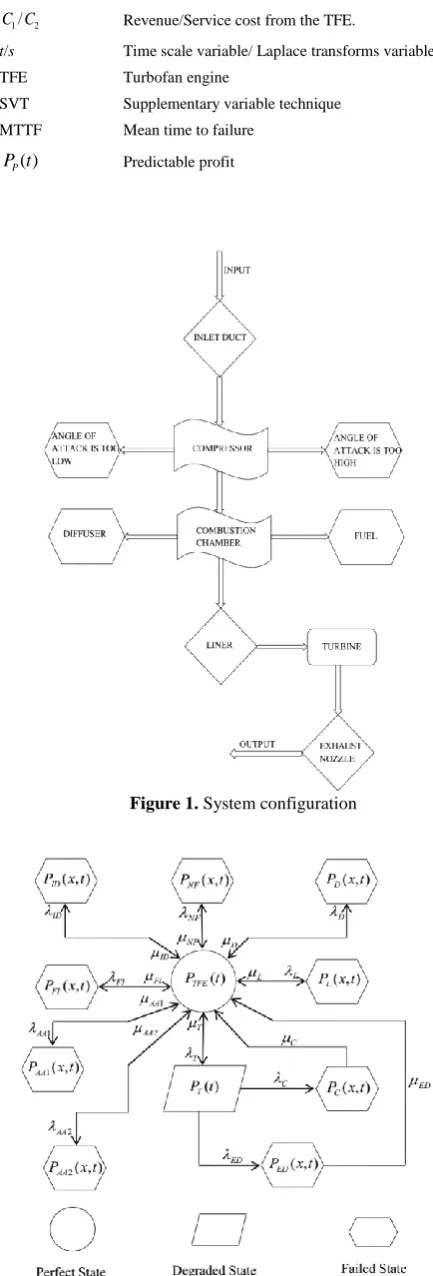
The configuration of TFE is shown in Figure 1. Based on the configuration of TFE a state transition diagram was developed as shown in Figure 2.
4. ASSUMPTIONS AND NOTATIONS
The following assumptions have been taken into account based on previous study:
(i) At t=0, the TFE is free from all types of defects. (ii) There is no delay in the maintenance action. (iii)Simultaneous failure of any two units is not
possible.
(iv)Average failure rates are taken to be constant. The following notations are used throughout the study.
) (t
PTFE
The state probability at time t when TFE is working with full efficiency.
) (t PT
The state probability at time t when TFE is in degraded state because of turbine failure.
) , (xt PL
The state probability at time t when TFE is not working because of Liner failure.
) , (xt PD
The state probability at time t when TFE is not working because of diffuser failure.
) , (xt PNF
The state probability at time t when TFE is not working because of non-availability of fuel.
) , (xt PID
The state probability at time t when TFE is not working because of inlet duct failure.
) , (xt PFI
The state probability at time t when TFE is not working because of fuel injector failure.
) , ( 1 xt
PAA
The state probability at time t when TFE is not working because of the angle of attack is too low.
) , (
2 xt PAA
The state probability at time t when TFE is not working because of the angle of attack is too high.
) , (xt PED
The state probability at time t when TFE is not working because of exhaust duct failure.
) , (xt PC
The state probability at time t when TFE is not working because of compressor failure.
T C ED
AA AA FI
ID NF D L
/ /
/ / / /
/ / /
2 1
Failure rate of Liner/Diffusor/Non-availability of fuel/Inlet duct/Fuel injector/Angle of attack too low/Angle of attack too high/Exhaust duct/Compressor/Turbine.
T C ED
AA AA FI
ID NF D L
/ /
/ / / /
/ / /
2 1
Repair rate of Liner/Diffusor/Non-availability of fuel/Inlet duct/Fuel injector/Angle of attack too low/Angle of attack too high/Exhaust duct/Compressor/Turbine.
2 1/C
C Revenue/Service cost from the TFE.
t/s Time scale variable/ Laplace transforms variable. TFE Turbofan engine
SVT Supplementary variable technique
MTTF Mean time to failure
) (t
PP Predictable profit
Figure 1. System configuration
5. MATHEMATICAL ORIGINATION AND SOLUTION OF THE PROBLEM
Based on state transition diagram (Figure 2) of TFE, the following systems of intro-differential equation are generated:
i i i T T TFE AA AA T ID NF D FI L dx t x P t P t P t 0 2 1 ) , ( ) ( ) ( (1)where i= L, FI, D, NF, ID, AA1, AA2, C, ED respectively.
) ( )
(t P t
P
t ED C T T T TFE
(2) 0 ) , ( t x P x
t ID ID (3)
0 ) , ( t x P x
t NF NF (4)
0 ) , ( t x P x
t D D (5)
0 ) , ( t x P x
t FI FI (6)
0 ) , ( t x P x
t L L (7)
0 ) , ( 1
1
t x P x
t AA AA (8)
0 ) , ( 2
2
t x P x
t AA AA (9)
0 ) , ( t x P x
t ED ED (10)
0 ) , ( t x P x
t C C (11)
Boundary conditions: ) ( ) , 0
( t P t
Pi i j (12)
where i= ID, NF, D, FI, L, AA1, AA2, C, ED
j= TFE, TFE, TFE, TFE, TFE, TFE, T, TFE, T respectively. Initial condition: 0 , 0 0 , 1 ) ( t t t
PTFE (13)
Taking Laplace transform from Equation (1-12), one can obtain:
i i i T T TFE AA AA T ID NF D FI L dx s x P s P s P s 0 2 1 ) , ( ) ( 1 ) ( (14)where i= L, FI, D, NF, ID, AA1, AA2, C, ED respectively.
sEDCT
PT(s)TPTFE(s) (15)0 ) , ( s x P s
x ID ID (16)
0 ) , ( s x P s
x NF NF (17)
0 ) , ( s x P s
x D D (18)
0 ) , ( s x P s
x FI FI (19)
0 ) , ( s x P s
x L L (20)
0 ) , ( 1
1
s x P s
x AA AA (21)
0 ) , ( 2
2
s x P s
x AA AA (22)
0 ) , ( s x P s
x ED ED (23)
0 ) , ( s x P s
x C C (24)
Boundary conditions: ) ( ) , 0
( s P s
Pi i j (25)
where i= ID, NF, D, FI, L, AA1, AA2, C, ED
j= TFE, TFE, TFE, TFE, TFE, TFE, T, TFE, T respectively.
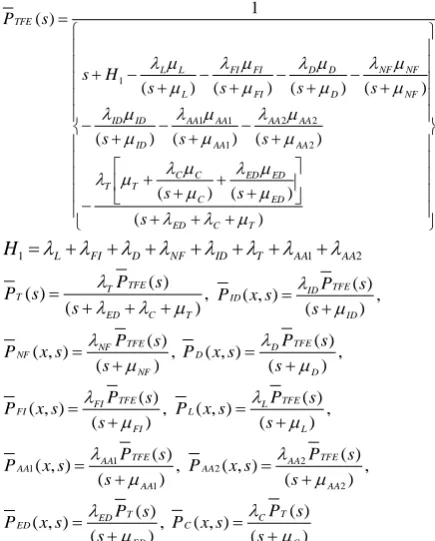
) ( ) ( ) ( ) ( ) ( ) ( ) ( ) ( ) ( ) ( 1 ) ( 2 2 2 1 1 1 1 T C ED ED ED ED C C C T T AA AA AA AA AA AA ID ID ID NF NF NF D D D FI FI FI L L L TFE s s s s s s s s s s H s s P 2 1
1 L FI D NF ID T AA AA
H
, ) ( ) ( ) ( T C ED TFE T T s s P s P , ) ( ) ( ) , ( ID TFE ID ID s s P s x P , ) ( ) ( ) , ( NF TFE NF NF s s P s x P , ) ( ) ( ) , ( D TFE D D s s P s x P , ) ( ) ( ) , ( FI TFE FI FI s s P s x P , ) ( ) ( ) , ( L TFE L L s s P s x P , ) ( ) ( ) , ( 1 1 1 AA TFE AA AA s s P s x P , ) ( ) ( ) , ( 2 2 2 AA TFE AA AA s s P s x P , ) ( ) ( ) , ( ED T ED ED s s P s x P ) ( ) ( ) , ( C T C C s s P s x P
From the state transition diagram the working (i.e. perfect/degraded) state and failed state probabilities of the TFE are given as:
) ( ) ( )
(s P s P s
Pup TFE T (26)
) , ( ) , ( ) , ( ) , ( ) , ( )
(s P xs P xs P xs P xs P xs
Pdown ID NF D FI L
) , ( ) , ( ) , ( ) , ( 2
1 xs P xs P xs P x s
PAA C AA ED
(27)
6. NUMERICAL COMPUTATION
6. 1. Availability The availability of TFE can be obtained by taking inverse Laplace transform of Equation (26) as:
) 1 )( 1 ( ) 1 ( ) ( 1
2
C ED AA T ID AA D FI L NF T C ED upt P ) ( ) 1 ( ) ( ) ( 2 1 2 1 1 2 1 2 1 2 1 C ED D AA AA T ID NF FI L D AA AA T ID NF FI L t D AA AA T ID NF FI L NF AA ID AA D FI L C ED T AA AA L FI D NF ID e ) 1 )( ( ) ( 2 1 1 C ED C ED D AA AA T ID NF FI L t C ED T C ED e (28)
Now put the value of various failure rates as λNF=0.01,
λD=0.01, λFI=0.06, λL=0.05, λAA1=0.14, λAA2=0.14,
λT=0.02, λED=0.05, λC=0.14, λID=0.05, and repair rate as:
µID= µNF= µD= µFI= µL= µAA1= µAA2= µT= µED= µC=1in
Equation (28), one can obtain availability of the system as: t t up e e t P 19 . 1 48 . 1 7 0110113010 . 0 3019571296 . 0 6 9 68703156 . 0 ) ( (29)
Now varying time t in Equation (29), one can get Table 1 and Figure 3 for availability of TFE.
6. 2. Reliability For reliability evaluation of TFE take the value of different failure rates as λNF=0.01,
λD=0.01, λFI=0.06, λL=0.05, λAA1=0.14, λAA2=0.14,
λT=0.02, λED=0.05, λC=0.14, λID=0.05, and repair rate as
µID= µNF= µD= µFI= µL= µAA1= µAA2= µT= µED= µC=0 in
Equation (26) than taking inverse Laplace transform, the reliability of the system is given as:
) 48 . 0 ( ) 19 . 1 ( 028169017 . 1 8 0281690140 . 0 )
( t t
e e
t
R (30)
Now changing time unit in Equation (30), Table 2 and Figure 4 are obtained for availability of TFE.
TABLE 1. Availability of TFE vs. Time
Figure 3. Availability of TFE vs. Time
0 2 4 6 8 10
0.65 0.70 0.75 0.80 0.85 0.90 0.95 1.00 1.05 A v ai la b il it y P u p (t ) Time(t)
Time unit Availability P (t) up
0 1.00000
1 0.75911
2 0.70369
3 0.69090
4 0.68793
5 0.68724
6 0.68708
7 0.68704
8 0.68703
9 0.68703
6. 3. MTTF The MTTF of the TFE is evaluated by taking all repairs equal to zero in Equation (26) and taking s tends to zero, the MTTF of the system is given as:
) 1 )(
( ID NF D FI L AA1 AA2 T ED C
T
MTTF
) (
1
2
1 AA T
AA L FI D NF
ID
(31)
Now taking failure rates from 0.01 to 0.09 one by one in Equation (31), the MTTF of TFE is obtained as given in Tables 3(a) and 3(b) and Figure 5.
Figure 4. Reliability of TFE vs. Time
Figure 5. MTTF vs. Failure rate of TFE
TABLE 2. Reliability of TFE vs. Time
Time unit Reliability R(t)
0 1.00000
1 0.62764
2 0.39107
3 0.24280
4 0.15049
5 0.09319
6 0.05769
7 0.03570
8 0.02209
9 0.01367
10 0.00846
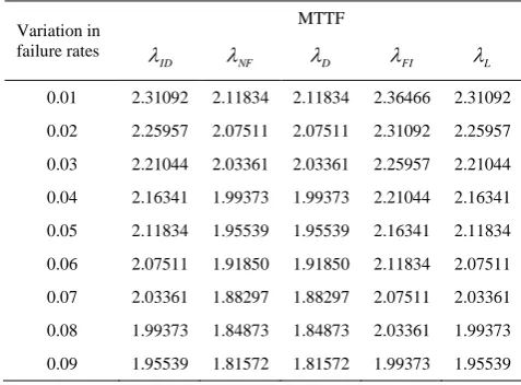
TABLE 3(a). MTTF vs. Failure rate of TFE
Variation in failure rates
MTTF
ID
NF D FI L
0.01 2.31092 2.11834 2.11834 2.36466 2.31092
0.02 2.25957 2.07511 2.07511 2.31092 2.25957
0.03 2.21044 2.03361 2.03361 2.25957 2.21044
0.04 2.16341 1.99373 1.99373 2.21044 2.16341
0.05 2.11834 1.95539 1.95539 2.16341 2.11834
0.06 2.07511 1.91850 1.91850 2.11834 2.07511
0.07 2.03361 1.88297 1.88297 2.07511 2.03361
0.08 1.99373 1.84873 1.84873 2.03361 1.99373
0.09 1.95539 1.81572 1.81572 1.99373 1.95539
TABLE 3(b). MTTF vs. Failure rate of TFE
Variation in failure rates
MTTF
1
AA
AA2 T ED C
0.01 2.90516 2.90516 2.14553 2.11956 2.12264
0.02 2.82446 2.82446 2.11834 2.11925 2.12227
0.03 2.74812 2.74812 2.09226 2.11894 2.12191
0.04 2.67580 2.67580 2.06722 2.11864 2.12155
0.05 2.60719 2.60719 2.04317 2.11834 2.12121
0.06 2.54201 2.54201 2.02003 2.11805 2.12087
0.07 2.48001 2.48001 1.99778 2.11776 2.12053
0.08 2.42096 2.42096 1.97634 2.11748 2.12020
0.09 2.36466 2.36466 1.95569 2.11720 2.11988
6. 4. Sensitivity Analysis
6. 4. 1. Sensitivity of Reliability The sensitivity analysis of the TFE for reliability can be done by differentiating the reliability expression with respect to various failure rates and then taking the values of failures as λNF=0.01, λD=0.01, λFI=0.06, λL=0.05,
λAA1=0.14, λAA2=0.14, λT=0.02, λED=0.05, λC=0.14,
λID=0.05,the values of ,
) ( ID
t R
, ) (
T
t R
, ) ( ED
t R
, ) (
D
t R
, ) (
FI
t R
, ) (
L
t R
(),
1 AA
t R
, ) (
2 AA
t R
C t R
()
, NF
t R
()
are
obtained. Now varying time unit t in these partial derivatives, we get Tables 4(a) and 4(b) and corresponding Figure 6 for sensitivity of reliability as:
0 2 4 6 8 10
0.0 0.2 0.4 0.6 0.8 1.0
R
el
ia
bi
li
ty
R
(t
)
Time(t)
0.02 0.04 0.06 0.08 0.10
1.8 2.0 2.2 2.4 2.6 2.8 3.0
C E D
&
T
L ID
&
F I
D N F
&
2 1& A A A A
M
T
T
F
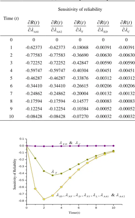
TABLE 4(a). Sensitivity of reliability
Time (t)
Sensitivity of reliability
ID t R
()
NF
t R
()
D t R
()
FI t R
()
L t R
()
0 0 0 0 0 0
1 -0.62373 -0.62373 -0.62373 -0.62373 -0.62373
2 -0.77583 -0.77583 -0.77583 -0.77583 -0.77583
3 -0.72252 -0.72252 -0.72252 -0.72252 -0.72252
4 -0.59747 -0.59747 -0.59747 -0.59747 -0.59747
5 -0.46287 -0.46287 -0.46287 -0.46287 -0.46287
6 -0.34410 -0.34410 -0.34410 -0.34410 -0.34410
7 -0.24862 -0.24862 -0.24862 -0.24862 -0.24862
8 -0.17594 -0.17594 -0.17594 -0.17594 -0.17594
9 -0.12254 -0.12254 -0.12254 -0.12254 -0.12254
10 -0.08428 -0.08428 -0.08428 -0.08428 -0.08428
TABLE 4(b). Sensitivity of reliability
Time (t)
Sensitivity of reliability
1 ) (
AA t R
2 ) (
AA t R
T t R
()
ED t R
()
C t R
()
0 0 0 0 0 0
1 -0.62373 -0.62373 -0.18068 -0.00391 -0.00391
2 -0.77583 -0.77583 -0.36690 -0.00630 -0.00630
3 -0.72252 -0.72252 -0.42847 -0.00590 -0.00590
4 -0.59747 -0.59747 -0.40304 -0.00451 -0.00451
5 -0.46287 -0.46287 -0.33876 -0.00312 -0.00312
6 -0.34410 -0.34410 -0.26615 -0.00206 -0.00206
7 -0.24862 -0.24862 -0.20004 -0.00132 -0.00132
8 -0.17594 -0.17594 -0.14577 -0.00083 -0.00083
9 -0.12254 -0.12254 -0.10384 -0.00052 -0.00052
10 -0.08428 -0.08428 -0.07270 -0.00032 -0.00032
Figure 6. Sensitivity of reliability
6. 4. 2. Sensitivity of MTTF For computing sensitivity analysis of the TFE with respect to MTTF, differentiate Equation (30) with respect to various failure rates and then setting the values of failure rates as λNF=0.01, λD=0.01, λFI=0.06, λL=0.05, λAA1=0.14,
λAA2=0.14, λT=0.02, λED=0.05, λC=0.14, λID=0.05, the
values of NF
MTTF
( )
, ID
MTTF
( )
, D
MTTF
( )
, C
MTTF
( )
,
T
MTTF
( )
,
1
) (
AA
MTTF
,
2 ) (
AA MTTF
, ED
MTTF
( )
, L
MTTF
( )
, FI
MTTF
( )
. Now varying the failure rates as 0.01, 0.02,
0.03, 0.04, 0.05, 0.06, 0.07, 0.08, 0.09 in these partial derivatives of MTTF, Table 5(a) and 5(b) and corresponding Figure 7 give the sensitivity of MTTF as:
TABLE 5(a). Sensitivity of MTTF
Failure rates
Sensitivity of MTTF
ID
MTTF
( )
NF
MTTF
( )
D
MTTF
( )
FI
MTTF
( )
L
MTTF
( )
0.01 -5.25210 -4.41322 -4.41322 -5.49922 -5.25210
0.02 -5.02126 -4.23493 -4.23493 -5.25210 -5.02126
0.03 -4.80532 -4.06722 -4.06722 -5.02126 -4.80532
0.04 -4.60301 -3.90929 -3.90929 -4.80532 -4.60301
0.05 -4.41322 -3.76037 -3.76037 -4.60301 -4.41322
0.06 -4.23493 -3.61981 -3.61981 -4.41322 -4.23493
0.07 -4.06722 -3.48699 -3.48699 -4.23493 -4.06722
0.08 -3.90929 -3.36134 -3.36134 -4.06722 -3.90929
0.09 -3.76037 -3.24236 -3.24236 -3.90929 -3.76037
TABLE 5(b). Sensitivity of MTTF
Failure rates
Sensitivity of MTTF
1
) (
AA
MTTF
2
) (
AA
MTTF
T
MTTF
( )
ED
MTTF
( )
C
MTTF
( )
0.01 -8.30046 -8.30046 -2.77702 -0.03150 -0.03708
0.02 -7.84573 -7.84573 -2.66252 -0.03096 -0.03639
0.03 -7.42736 -7.42736 -2.55495 -0.03043 -0.03572
0.04 -7.04159 -7.04159 -2.45378 -0.02992 -0.03506
0.05 -6.68511 -6.68511 -2.35849 -0.02942 -0.03443
0.06 -6.35504 -6.35504 -2.26865 -0.02893 -0.03381
0.07 -6.04882 -6.04882 -2.18385 -0.02845 -0.03321
0.08 -5.76421 -5.76421 -2.10372 -0.02799 -0.03263
0.09 -5.49922 -5.49922 -2.02791 -0.02754 -0.03206
0 2 4 6 8 10
-0.8 -0.7 -0.6 -0.5 -0.4 -0.3 -0.2 -0.1 0.0 0.1
C E D
&
2 1 &
, , , ,
, N F D F I L A A A A ID
T
Se
ns
it
iv
it
y o
f R
el
ia
bi
li
ty
Figure 7. Sensitivity of MTTF
6. 5. Predictable Profit The predictable profit for
the considered system in [0, t) is given as [13, 14].
t up
P t C P tdt tC P
0
2
1 ()
)
( (32)
Now using Equation (28) in (32), and putting the value of different failure rates as λNF=0.01, λD=0.01, λFI=0.06,
λL=0.05, λAA1=0.14, λAA2=0.14, λT=0.02, λED=0.05,
λC=0.14, λID=0.05, the predictable profit function is
given as:
t C e
e t
C t P
t
t
p 1.19 2
48 . 1
1
2132782818 .
0 85 0092531941 .
0
2040250876 .
0 6870315694 .
0 )
(
(33)
Setting revenue C1= 1 and varying service cost C2 as
0.1, 0.2, 0.3, 0.4, 0.5, 0.6 respectively then varying time scale t in Equation (33), Table 6 and correspondingly Figure 8 give predictable profit for TFE.
7. RESULTS and DISCUSSION
This research work investigated a turbofan engine in context of Markov modeling. The findings on the availability of TFE are shown in Figure 3. It reflects that the availability of the TFE decreases smoothly as time passes and after a specific time span it becomes constant. Further, the reliability of the system is shown in Figure 4; it shows that the reliability of TFE decreases hurriedly as compared to availability. The difference between Figure 3 and Figure 4 shows the importance of a good maintenance policy. Figure 5 shows the graph of MTTF vs. failure rates. From this graph, it is observed that the MTTF of TFE is highest when the angle of attack is too low, and angle of attack is too high and lowest for the failure rates of diffuser and non-availability of fuel.
Figure 8. Predictable profit vs. time
TABLE 6. Predictable profit vs. time
Time unit
Predictable profit Pp(t)
C2=0.1 C2=0.2 C2=0.3 C2=0.4 C2=0.5 C2=0.6
0 0 0 0 0 0 0
1 0.75105 0.65105 0.55105 0.45105 0.35105 0.25105
2 1.37591 1.17591 0.97591 0.77591 0.57591 0.37591
3 1.97170 1.67170 1.37170 1.07170 0.77170 0.47170
4 2.56077 2.16077 1.76077 1.36077 0.96077 0.56077
5 3.14828 2.64828 2.14828 1.64828 1.14828 0.64828
6 3.73543 3.13543 2.53543 1.93543 1.33543 0.73543
7 4.32249 3.62249 2.92249 2.22249 1.52249 0.82249
8 4.90952 4.10952 3.30952 2.50952 1.70952 0.90952
9 5.49656 4.59656 3.69656 2.79656 1.89656 0.99656
10 6.08359 5.08359 4.08359 3.08359 2.08359 1.08359
0.02 0.04 0.06 0.08 0.10
-9 -8 -7 -6 -5 -4 -3 -2 -1 0
C ED
&
2 1& AA AA
FI
L ID
NF& D
&
T
S
en
si
ti
v
it
y
o
f
M
T
T
F
Variation in Failure Rates
0 2 4 6 8 10
0 1 2 3 4 5 6 7
6 . 0
2 C
5 . 0 2
C
4 . 0
2 C
3 . 0
2 C
2 . 0
2 C
1 . 0
2 C
E
xp
ec
te
d
P
ro
fi
t
It means that the maintenance team must pay more attention to the failure rates on these subunits. Figure 6 shows the graph of sensitivity of reliability vs. time. It is observed from this graph that system reliability is most sensitive with respect to the failure rate of inlet duct, non-availability of fuel, diffusor, fuel injector and liner, angle of attack is too low and angle of attack is too low. So in order to make TFE more reliable one has to control these failure rates. Figure 7 shows the graph of sensitivity of MTTF vs. failure rates. It reflects that the MTTF of TFE is most sensitive when the angle of attack is too low/too high. So in order to make system MTTF least sensitive we have to control the angle of attack. The predictable profit from TFE is shown in Figure 8. It shows the variation in predictable profit with respect to system service cost and time. The graph reflects that the predictable profit from the system decreases as service cost increases. So in order to enhance the profit one has to control the service cost of TFE.
8. CONCLUSION
In this paper, the reliability measures of a turbofan engine is discussed with the help of Markov process and supplementary variable techniques, for evaluating their various reliability characteristics. Based on results and discussion section, it is concluded that the MTTF of TFE is highest with respect to the angle of attack when it is too low and too high. In addition, system reliability is most sensitive with respect to the failure rate of inlet duct, non-availability of fuel, diffusor, fuel injector and liner when angle of attack is too low and too high. Therefore, to make TFE more reliable one has to control these failure rates. The MTTF of TFE is most sensitive when the angle of attack is too low/too high. Therefore, to make system MTTF least sensitive we have to control the angle of attack. It asserts that the finding of this paper is highly beneficial for the concern management of the TFE.
9. REFERENCES
1. Liu, F. and Sirignano, W. A., "Turbojet and turbofan engine performance increases through turbine burners", Journal of Propulsion and Power, Vol. 17, No. 3, (2001), 695-705. 2. Minato, R., Oota, T., Fukutomi, K., Tanatsugu, N., Mizobata,
K., Kojima, T. and Hiroaki, K., "Development of counter rotating axial fan turbojet engine for supersonic unmanned plane", in 43rd AIAA/ASME/SAE/ASEE Joint Propulsion Conference & Exhibit, (2007).
3. Braig, W., Schulte, H. and Riegler, C., "Comparative analysis of the windmilling performance of turbojet and tbrbofan engines",
Journal of Propulsion and Power, Vol. 15, No. 2, (1999), 326-333.
4. Gorji, M., Kazemi, A. and Ganji, D., "Uncertainties due to fuel heating value and burner efficiency on performance functions of turbofan engines using monte carlo simulation", International Journal of Engineering-Transactions A: Basics, Vol. 27, No. 7, (2013), 1139-1148.
5. Parrett, A. and Eversman, W., "Wave envelope and finite element approximations for turbofan noise radiation in flight",
American Institute of Aeronautics and Astronautics Journal, Vol. 24, No. 5, (1986), 753-760.
6. Turan, O., "Effect of reference altitudes for a turbofan engine with the aid of specific–exergy based method", International Journal of Exergy, Vol. 11, No. 2, (2012), 252-270.
7. Stone, J. R., "Flight effects on exhaust noise for turbojet and turbofan engines—comparison of experimental data with prediction", The Journal of the Acoustical Society of America, Vol. 60, No. S1, (1976), S113-S113.
8. Thomas, R. H., Burdisso, R. A., Fuller, C. R. and O'Brien, W. F., "Active control of fan noise from a turbofan engine",
American Institute of Aeronautics and Astronautics Journal, Vol. 32, No. 1, (1994), 23-30.
9. Moller, J. and Adams, R., "Performance deterioration of a turbofan and a turbojet engine upon exposure to a dust environment", Journal of Engineering for Gas Turbines and Power, Vol. 109, No. 3, (1987), 336-343.
10. Danforth, E., "Distortion-induced vibration in fan and compressor blading", Journal of Aircraft, Vol. 12, No. 4, (1975), 216-225.
11. Devereux, B. and Singh, R., "Use of computer simulation techniques to assess thrust rating as a means of reducing turbo-jet life cycle costs", in ASME 1994 International Gas Turbine and Aeroengine Congress and Exposition, American Society of Mechanical Engineers., (1994), V005T015A015-V005T015A015.
12. Ram M. and Chandna, R., "Reliability measures measurement under rule-based fuzzy logic technique", International Journal of Engineering, Transactions A: Basics, Vol. 28, No. 10, (2015), 1486-1492.
13. Ram, M. and Kumar, A., "Paper mill plant performance evaluation with power supply in standby mode", International Journal of Quality & Reliability Management, Vol. 32, No. 4, (2015), 400-414.
14. Kumar, A. and Ram, M., "Performance of marine power plant under generators, main switch board and distributed board failures", Journal of Marine Science and Application, Vol. 14, No. 4, (2015), 450-458.
15. Sadjadi, S., Makui, A., Zangeneh, E. and Mohammadi, S., "Reliability optimization for complicated systems with a choice of redundancy strategies (technical note)", International Journal of Engineering-Transactions A: Basics, Vol. 28, No. 10, (2015), 1476-1485.
16. Khanduja, R., Tewari, P. and Kumar, D., "Mathematical modeling and performance optimization for the digesting system of a paper plant", International Journal of Engineering-Transactions A: Basics, Vol. 23, No. 3&4, (2010), 215-226. 17. Gupta, S. and Tewari, P., "Performance modeling of power
generation system of a thermal plant", International Journal of Engineering, Vol. 24, No. 3, (2011), 239-248.
18. Kumar, A., Varshney, A. and Ram, M., "Sensitivity analysis for casting process under stochastic modelling", International Journal of Industrial Engineering Computations, Vol. 6, No. 3, (2015), 419-432.
Turbofan Engine Performance under Reliability Measures Approach
A. Kumara, R. Kumarb, M. Ramc
a Department of Mathematics, Lovely Professional University, Mathematics, Punjab, India b Department of Mechanical Engineering, Graphic Era University, Dehradun, India c Department of Mathematics, Graphic Era University, Dehradun, India
P A P E R I N F O
Paper history:
Received 17 October 2016
Received in revised form 21 January 2017 Accepted 09 February 2017
Keywords: Turbofan Engine Sensitivity Analysis Reliability Measures Maintenance Modeling Cost Analysis SVT
ديكچ ه
ا رد نی ون ،هلاقم ناگدنسی فلتخم لماوع ی
ار م هک ی ناوت ن درکلمع د کی ثات تحت ار نفوبروت روتوم ری
رارق دنهد سررب ی
دندرک ارب . ی ا نی ز ،راک ری اهدحاو ی زا فلتخم کی ارجم دننام نفوبروت روتوم ی
دورو ،ی ،شوب ،قارتحا هظفحم ،روسرپمک
بروت ،نی غ و زوزگا لزان هری
سررب دروم ی تفرگ رارق ناوتب ات
و یگژی اه ی مطا لباق نانی رط زا ار نآ فلتخم قی
ارف دنی
نکت و فوکرام کی
غتم ری ( لمکم
SVT
) درک ادیپ زم . تی لصا ی ا نی ا هلاقم نی زا هک تسا رط قی نیا م راک ی قد ناوت اقی اب و
دحاو /لماوع تقد ییاه
ب هک رتشی یور نفوبروت روتوم درکلمع درک ییاسانش ار دنراد ریثات
سررب زا سپ . ،ی
ا نی ن هجیت
دش لصاح نامز هک طسوتم واز تسکش هب هی
ب هلمح رتشی لوط رد درکلمع م خر نفوبروت روتوم ی
ا رب هولاع .دهد ،نی
طابنتسا نینچ یم
دوش هک نامز نیا تبسن ارجم تسکش خرن هب ی
دورو ی تن .تسا رت ساسح هجی
م ناشن ی هب هک دهد
هب روظنم هنی زاس ی ت راظتنا دروم دوس می
معت ری رادهگن و ی اب دی زه هنی سیورس اه شخب ی نفوبروت روتوم تسکش فلتخم
لرتنک دوش .