Please cite this article as: A. Toloei, H. Ramezi, Analysis of Transient Flow in the Case of Secondary Injection for Transient Vector Control, International Journal of Engineering (IJE), TRANSACTIONS C: Aspects Vol. 29, No. 6, (June 2016)
International Journal of Engineering
J o u r n a l H o m e p a g e : w w w . i j e . i r
Analysis of Transient Flow in the Case of Secondary Injection for Transient Vector
Control
A. Toloei*, H. Ramezi
Aerospace Department, Shahid Beheshti University, Tehran, Iran
P A P E R I N F O
Paper history:
Received 19 December 2015 Received in revised form 06 May 2016 Accepted 02 June 2016
Keywords: Fluid Mechanics Flow Field
Computational Fluid Dynamics Secondary Injection Thrust Vector Control Injection Angle Nozzle
A B S T R A C T
The purpose of this paper is to analyze the flow field structure in transient state and performance of secondary injection system for thrust vectoring in divergent section of a two-dimensional nozzle. Secondary injection for thrust vectoring in a two-dimensional nozzle is studied by solving three-dimensional Reynolds-averaged equations by means of fluent solver. Spalart-Allmaras model was used to model the fluid behavior near the walls. Density-based solver and explicit formulation are employed in the computational model. Results show that the solution of interfered field in the transient-state is more accurate than steady-state, especially in the initial injection. In addition, various testing showed that the maximum side force would be in the injection angle of twenty degrees and with increasing pressure ratio, we have more side force. At the end it was observed that by sketching the exit gases deviation according to time, we could be informed of desired secondary injection time in order to achieve required deviation around pitch axis, and the required force to achieve desired deviation angle. The innovation of this paper is the solution of interfered field in transient state, and of course the injection from the optimal point.
doi: 10.5829/idosi.ije.2016.29.06c.00
1. INTRODUCTION1
For controlling the rocket or spacecraft launcher or the spacecraft and satellites themselves which cannot exploit aerodynamic forces in outer atmosphere, Thrust Vector Control (TVC) is the only imaginable way. In addition, at the very beginning of the missiles launch period, especially heavy ones, because of low momentum dynamic forces are negligible. One way to prevent the deviation of missiles in these moments is the TVC. Conventional thrust vector control methods for solid fuel engines require the use of TVC for control under the above conditions. One of the ways used for solid fuel engines thrust vector control method from 1950s is called the secondary injection. In this way thrust vector is controlled by fluid injection from holes in the nozzle wall. The fluid injection from holes of the nozzle changes the nozzle’s boundary layer and thus the direction of exhaust gas from the nozzle and the
1*Corresponding Author’s Email: [email protected] (A. Toloei)
pressure distribution on the interior wall of the nozzle, therefore; the thrust vector will be changed. Even though in this method, unlike other methods, the system is simple but studying its behavior requires a lot of experience and experiments. It can say that a lot of studies has been carried out in the area of numerical simulation of Fields resulted from a jet entering into a main flow.
These studies include Letko showed that the secondary injection system with an injection of supersonic flow into the main flow, in compare to sonic flow injection, can achieve greater lateral thrust [1]. He also introduced a suction zone downstream of the injection orifice as a reducing factor on lateral force. By performing a series of calculations, he showed that by eliminating or reducing the suction zone, it is possible to increase the side force by about 13 percent. Several investigations have been carried out on the unsteady or start-up flow phenomena in nozzle. All of these work has been chiefly of an analytical nature with little quantitative experimental corroboration. To improve the
results, an analytical and experimental study of these phenomena was made at Lehigh University. The particular problem investigated involved a two-dimensional nozzle of hyperbolic contour attached to a large reservoir initially containing a stagnant pressurized gas. Gas flow was initiated through the bursting of a membrane at the nozzle exit, and the gas is discharged directly into the surroundings by Benjamin [2]. Gauss experimentally studied effective parameters in secondary injection system’s performance in a two dimensional nozzle, including: temperature, stagnation pressure, molecular weight, secondary fluid specific heat, basic flow’s Mach number, width of the inlet, and injection angle. He proposed relationships to estimate system’s performance based on his observations [3]. In this study, the numerical simulation of unsteady transonic flow in diffusers was investigated. Forced and self-excited oscillation of transonic flows in two-dimensional diffusers was numerically simulated using the compressible Reynolds-averaged Navier-Stokes equations.
Depending on the shock strengths and the area ratios, the character of the flows ranged from fully attached to largely separated. In the case of forced oscillations, a harmonic pressure wave was prescribed at the exit plane. Data solutions over several cycles of quasi periodic motion were analyzed by spectral methods. Comparisons of computed and experimental results generally gave good to very good agreement for the forced oscillation cases and fair to good agreements for the self-excited oscillation cases has been done by Meng Sing- Liou et al. [4]. A procedure used to calculate the effects of rocket motor rotation on the subsonic/transonic flow field in axisymmetric rocket motor nozzle is presented here. The governing equations for the unsteady three-dimensional flow of an ideal, inviscid fluid in thermodynamic equilibrium are derived in a non-inertial reference frame. The governing
equations are integrated numerically using
McCormack’s explicit finite difference method. The boundary conditions are applied using Kentzer’s method by Jeffrey J. Brown and et al. [5].
In 1988 behavior of shock waves in unsteady unviscous transonic flow in nozzle was studied by Strada [6]. He explained that these transient conditions can be because of combustion instabilities or changes in power settings, among other reasons. Two techniques have been used to handle this type of problem: similarity transformations and asymptotic expansion.
This study examines the performance of an
axisymmetric nozzle which was designed with a Mach number of 8. A free piston-driven shock tube was used to supply the nozzle with temperature,
high-pressure test gas. Performance was assessed by measuring pitot pressures across the exit plane of the nozzle and, was examined over the range of operating conditions; the nozzle produced satisfactorily test flows by P.A.Jacobs [7].
Using images of the interfered field flow, penetration depth of injected jet was studied by Gruber et al. [8]. They examined effects of three types of orifices: circular, oblique circular and elliptical. Their study showed that due to the reduction in lateral momentum, jet penetration depth in circular and elliptical orifices is more in compared to oblique orifices. They also observed that in elliptical injectors, secondary fluid flow propagates faster in the lateral direction. Using the details of the flow, they also proposed a relationship for depth of the penetration of the secondary [8]. The space-time conservation
element/solution element (CE/SE) method in
conjunction with an unstructured mesh generator is applied to solve unsteady Navier-Stokes (N-S) rocket nozzle flows.
The space-time CE/SE method considers space and time as a single entity, preserves both local and global flux conservation in the solution procedure, and provides accurate, unsteady analysis results for both the N-S (viscous) and the Euler (inviscid) nozzle flows. No computational difficulty is encountered with the unstructured mesh using high-aspect-ratio triangular elements in the viscous boundary layer. Detailed calculations have been carried out for over expanded flows inside the JPL axisymmetric, convergent-divergent nozzle by I-Shih Chang [9]. Unsteady solution to the Navier-Stokes for the flow in the nozzle to simulate the flow inside the nozzle and secondary injection has been studied by I-Shih Chang and et al. [10].
In this study we follow this procedure: in section 2 we describe Secondary Injection for Thrust Vector Control (SITVC). Section 3 is dedicated to explaining the problem. For section 4 governing equations for flow, and in section 5 implemented turbulent model is presented. In section 6 generated mesh is explained and finally in section 7 we have presented the obtained results.
2. THE PERFORMANCE OF SITVC AND THE EFFECTIVE PARAMETERS
Figure 1 shows the divergence of the current flow due to the jet injection. By respect to that, the thrust Vector of deflection angle is equal to
:
Figure 1. The axial thrust force, lateral thrust and thrust vector divergence angle [11]
In Equation (1), is the resultant force of all of those that are laterally applying on the nozzle wall and is called the total lateral thrust. Also, is the axial thrust, In SITVC the symmetry of the pressure field on the nozzle wall will disturb due to the interference of the secondary jet, In this system, the total lateral thrust is equal to:
(2)
In Equation (2), 𝛿 is the change in secondary jet during the injection inside the main flow and is the pressure term of the lateral thrust due to the asymmetry of pressure distribution on the nozzle wall. is the induced or interference lateral thrust. This term approximately forms the 80 to 90 percent of the total lateral thrust and is calculated by integrating the pressure on the nozzle wall as following:
(3)
∫ ∫
In Equation (3), is the pressure on the internal nozzle wall, is the atmosphere pressure on the external nozzle wall, is the radius on any arbitrary point on the wall and and z are the angular and axial coordinates on cylindrical coordinate axes, respectively. Due to Equation (3) and to compute the interference lateral thrust, it is necessary to calculate the flow field inside the nozzle and also to determine the pressure distribution on the internal wall.
In SITVC, the ratio of mass flow rate of the secondary flow to the main flow and also the ratio of the lateral thrust to the axial thrust is defined as (4) and (5), respectively:
(4) Ψ ̇ ̇
(5) 𝜙
3. THE PROBLEM EXPLANATION, THE
PROCEDURE AND ASSUMPTIONS
One way of controlling the thrust vector is the Secondary injection that works based on changes in the
divergent section of the nozzle. The method of secondary injection of hot gas is lighter in comparison with the mechanical methods due to the simplicity and lack of moving parts and also has fewer costs of productions and maintenance. So, the goal of doing this project is solving the transient field in the nozzle considering the secondary injection. This project is done based on this fact that in the initial moments of injecting the flow characteristics in each point is changing with time, the forming field must be analyzed in the transient mode, so solving the field in the transient field will cause more exact results than in the steady mode and is closer to what happens in reality. Hence, this will inform the instantaneous changes in the lateral and axial thrusts, divergence of the outlet gasses with time and as a consequence, the divergence of the missile, itself. So, in general we can say that investigating the construction of the flow and the performance of a convergence-divergence nozzle along with the secondary injection in the transient mode will lead to obtaining the output parameters which are equating with the real ones.
The assumptions made thorough this paper are listed below:
The air is considered as ideal gas.
The injected fluid is the same as the main fluid.
The flow is considered to be isentropic.
The effects of the gravity are neglected.
The nozzle is considered to be cylindrical and two dimensional.
4. THE GOVERNING EQUATION OF THE FLOW
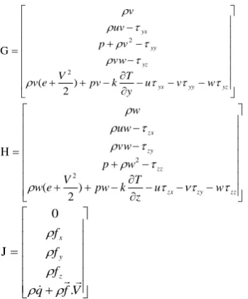
Solving the complete set of Navier-Stokes equations are the final goal of numerical simulation of fluid, we can obtain these equations by applying the stresses and rate of strain in the equations of motion. The Navier-Stokes equations consist of five sets of equations, mass conservation, momentum conservation in three coordinates, and energy conservation equations. The conservative form of Navier-Stokes equations in the Cartesian coordinates axes are as following:
(6) J
z H y G x F t
U
The parameters U, F, G, H and J could be obtained as:
w v u x T k pu ) 2 V e ( u
uw uv u p
u
F
) 2 V e (
w v u
U
xz xy xx 2
xz xy xx 2
2
) 2 ( G 2 2 yz yy yx yz yy yx w v u y T k pv V e v vw v p uv v ) 2 ( H 2 2 zz zy zx zz zy zx w u z T k pw V e w w p vw uw w . 0 J V f q f f f z y x
In the above equations, is the density, u is the velocity in x-direction, v is the velocity in y-direction, w is the velocity in z-direction, V the total speed, e the internal energy, p the pressure, , and are the body forces in x, y and z directions, respectively and ̇ is the rate of the volumetric thermal in the element per unit of mass, added. The only extra parameters required are the viscosity equation and thermal conductance with pressure and temperature which are usually calculated from the experimental measurements. Due to the turbulence form of the flow in the problem of secondary injection, the turbulence models are being used in the simulations. The turbulence model is discussed in the next section.
5. TURBULENCE MODEL USED IN THIS STUDY
Considering complex flow in regions around injected jet, and also the lack of exact knowledge about kinds and values of parameters affecting key characteristics of the flow, it is necessary to use a proper turbulence model for numerical solution. Obviously, there is no single turbulence model which can solve all kind of engineering problems. Choosing an appropriate model amongst available models depends on:
The flow mechanism ruling the problem
Whether there are multiple different flow regimes together or not
How much accuracy is needed
Calculating tools at hand (including RAM and CPU)
Required time in order to reach reasonable solution Among available turbulence models, we choose one-equation Spalart-Allmaras model. Of course it is
possible to use other models like k-ε and etc. In this study, but it doesn’t make a difference in flow pattern because all extracted phenomena are identical in these two models, and we have maybe just small differences in scale and amount of phenomena’s [16]. Considering above calculations, we use Spalart-Allmaras model in order for YPlus of walls to reach order one. In using this model for simulation, if for any reason proper amount of elements are not used near the walls, Fluent will compensate the lack of proper elements using available function. Furthermore, this model has a less sensibility to calculational errors originated from elemental deformation of mesh. This model is a one-equation model which has been design for Aerospace application. This model solves the transfer equation for eddy kinematic viscosity and without calculation of length scale relating to shear layer thickness. Transitive variable in Spalart-Allmaras model is velocity that has been modeled by kinematic viscosity in regions that hasn’t been affected by strong viscous effect in regions near wall.
6. MESH GENERATE
Generating a suitable computational mesh in modeling of phenomena’s into the flow field is very important. Considering complex nature of flow field including impact shock-to-shock and shock-to-wall, this importance is more understandable. Hence, the issue of choosing a proper network is an important part of the study. Computational mesh was generated by Gambit and its mesh structure was quad. Choosing a structured mesh gives us a more accurate solution than unstructured mesh. Then, generated mesh was transferred to Tgrid. Finally, the process of mesh generation was completed by generation of volumetric mesh in Tgrid.
6. 1. Independence of the Solution from Generated Mesh In order to prevent errors originated from the type of network, study of independence of solution from mesh carried out by three ways. We can see the characteristics of studied mesh in Table 1.
The results for pressure on upper and lower walls, thrust of main nozzle, and lateral force out of secondary injection are shown in Table 2.
As we see in Table 2:
Difference in values between network 1 and 2 is %1.499, and for network 2 and 3 is %1.0566.
TABLE 1. Evaluating the sensibility of studied mesh
The number of nodes
Number of pages
Number of cells
Number of grid
35388 70332 34945 1
54280 108016 53737 2
82044 163349 81306 3
Number of grid 3 Number of grid 2
Number of grid 1
Figure 2. Generated meshon the plane of symmetry
TABLE 2.Comparison of results for different networks
Pupper
wall(pa)
Pdown
wall(pa)
Fp(N) Fs(N) Number of
grid
306432/63 376714/16 41442/9 2826/07 1
305618/34 372124/63 41467/6 2783/81 2
304554/78 370463/19 41475/4 2754/3 3
Differences of pressure values for lower wall between all three networks are less than %1.
Difference of axial thrust value between network 1 and 2 is less than %1 and between 2 and 3 values is less than %2.
Considering the fact that there is no significant difference for the results between network 2 and 3, and also considering fewer cell numbers, we choose network 2 for carrying out the calculations.
7. RESULTS
The location for secondary injection was determined in study carried out by Rohani and Tolouei [12]. This specific point gives us maximum lateral thrust and minimum loss in axial thrust. So, according to [12] distance of injection point from throat was chosen 0.11m. Table 3 shows conditions for main flow and injection point. Figures 3 and 4 demonstrate the variations for axial and lateral thrust.
TABLE 3. Input conditions for carried out tests
Static pressure (kpa)
Stagnation temperature(K)
Mach number of entrance flow
Main
flow Orifice
Main
flow Orifice
Main
flow Orifice
700 330 300 300 1
Corresponding to the studied
subject
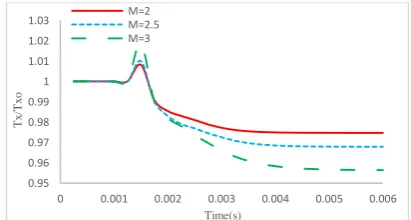
The time of calculations is 0.006 sec including 0.0001 sec that we do not have injection. An important factor in choosing this time span is time required to run the simulation. Since the simulation is carried out for transient state, running the simulation would take long time. Of course if we run the simulation by a supercomputer, time required would be much less than normal computers. Of course after some time of simulation, the solution would become steady and therefore increasing the time span would become ineffective. As we see in following figure, at first that there is no injection, axial thrust s maximum. As soon as we have injection, at the very beginning -because of small increase in mass flow rate- axial thrust is a little increased in comparison with the case we don’t have injection. Because it the beginning, the injected flow doesn’t have the strength enough to deviate main flow, its main effect is to add some mass flow to main axial flow -and thus in a little increase axial flow- rather than causing lateral flow. However, as we see in the following figures, even in this period of time, we have a little increase in lateral thrust, too. This slight increase in axial thrust doesn’t last long until injected flow gets the strength needed to cause the deviation of the main flow. Then, as soon as secondary flow reaches its maximum velocity and can deviate the main flow, axial thrust begins to decrease and in the same time lateral thrust increases. It’s worth mentioning here that the direction of injection is perpendicular to the lower wing. Table 4 summarizes percent increase and percent decrease of lateral and axial thrust in various injection Mach numbers.
Figure 3. Variation of axial thrust respecting time in different
Mach numbers
Figure 4. Variation of lateral thrust respecting time in
different Mach numbers 0.95
0.96 0.97 0.98 0.99 1 1.01 1.02 1.03
0 0.001 0.002 0.003 0.004 0.005 0.006
T
x
/T
x
o
Time(s)
M=2 M=2.5 M=3
0 0.02 0.04 0.06 0.08 0.1 0.12
0 0.002 0.004 0.006
T
y
/T
x
o
Time(s) M=2
TABLE 4. Percent increase and percent decrease of lateral and axial thrust in various injection Mach numbers.
Changed mach reduction Percent of
axial thrust
increase percent of lateral thrust
2 2/5 0/7 10/5
2 3 1/8 29/7
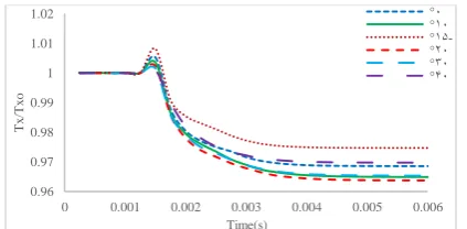
7. 2. Investigating Various Injection Mach Numbers in Different Injection Angles and Introducing Optimum Injection Angle At this moment, it is desired to find the optimum injection angle. For this end, different injection angles are exploited in a single injection with different Mach numbers and finally the optimum injection angle is introduced. Figure 5 and 6 show different injection angles in Mach number of 2. As it is clear in the figures below, the maximum injection angle of 20 degrees will result in the maximum lateral thrust. Although, in this optimum angle decrease in axial thrust is witnessed it is noteworthy that in secondary jet injection, the desired effect is to increase the lateral thrust. Moreover, increasing secondary jet injection angle from -15 degree (the primary jet injection angle) to 20 degree will increase the lateral thrust about 14.8 percent and on the other hand decrease the axial thrust about 1.1 percent. In other words, amount of decrease in axial thrust is negligible compared to amount of increase in lateral thrust.
Now, to validate the optimum injection angle introduced, different Mach numbers of 2.5 and 3 in different angles are studied. Figures 7 and 8 show various injection angles in Mach number of 2.5 and Figures 9 and 10 show various injection angles in Mach number of 3. Therefore, as it is shown the 20 degree injection angle is the optimum angle.
Altering the optimum angle from 20 degree to 30 or 40 degrees will result in decrease of the lateral thrust. Thus, Regardless of increasing or decreasing the injection angle from 20 degrees the lateral thrust will decrease.
Figure 5.Variation of axial thrust respecting time in different
angle and Mach numbers 2
Figure 6. Variation of lateral thrust respecting time in
different angle and Mach numbers 2
Figure 7.Variation of axial thrust respecting time in different
angle and Mach numbers 2/5
Figure 8.Variation of axial thrust respecting time in different
angle and Mach numbers 2/5
Figure 9. Variation of axial thrust respecting time in different
angle and Mach numbers 3
0.96 0.97 0.98 0.99 1 1.01 1.02
0 0.001 0.002 0.003 0.004 0.005 0.006
T
x
/T
x
o
Time(s)
0 °
10 °
-15 °
20 °
30 °
40 °
0 0.02 0.04 0.06 0.08 0.1 0.12
0 0.001 0.002 0.003 0.004 0.005 0.006
T
y
/T
x
o
Time(s)
0 °
10 °
-15 °
20 °
30 °
40 °
0.94 0.96 0.98 1 1.02
0 0.001 0.002 0.003 0.004 0.005 0.006
T
x
/T
x
o
Time(s)
0 °
10 °
-15 °
20 °
30 °
40 °
0 0.05 0.1 0.15
0 0.001 0.002 0.003 0.004 0.005 0.006
T
y
/T
x
o
Time(s)
0 °
10 °
-15 °
20 °
30 °
40 °
0.9 0.92 0.94 0.96 0.98 1 1.02 1.04
0 0.001 0.002 0.003 0.004 0.005 0.006
T
x/T
xo
Time(s)
0 °
10 °
-15 °
20 °
30 °
Figure 10. Variation of lateral thrust respecting time in different angle and Mach numbers 3
7. 3. Amount of Deviation of Outlet Gases Versus Time In this part, the deviation of outlet gases during the injection time will be depicted in degrees. To reach this goal, three different injection Mach numbers are used. However it should be noted that, since the optimum injection angle was found to be 20 degree, the deviation of outlet gases are studied in this angle. Figure 11 shows amount of deviation of outlet gases in different injection Mach numbers.As it is obvious in the figures, maximum deviation in Mach number of 3 is occurred in 20 degree angle, where maximum lateral thrust is acquired which was expected.
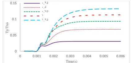
7. 4. Studying Various Pressure Ratios In this part, various pressure ratios ( ) of secondary jet is
analyzed in Mach number of 1 and the change of axial and lateral thrusts with time is witnessed with different pressure ratios. It should be noticed that the jet injection angle is considered -15 degree. Figures 12 and13 show various pressure ratios in Mach number of unity.
Figure 11. Deviation of outlet gases (degree) vs. time for
different Mach numbers
Figure 12. Variation of axial thrust respecting time in ratio
different pressure and Mach numbers 1
Figure 13.Variation of lateral thrust respecting time in ratio
different pressure and Mach numbers 1
As it is shown in the figure above, the lateral thrust will increase with increase in pressure ratio.
8. CONCLUSIONS
Studying the figures of simulation has yielded the following results:
More accurate results in compare to steady state solution are reached (since the characteristics of the interfered flow field in the primary moments of the injection are constantly changing and this change of characteristic is clearly shown in the 0 to 0.006 seconds of the simulation.)
Introduction of 20 degree angle as the optimum injection angle
The ability to show amount of deviation of outlet gases from nozzle during time (using this figure it is possible to estimate the required time to reach a certain amount of deviation. i.e. 0.006 seconds to reach 6 degree deviation if the deviation of 6 degree is required around pitch axis (in a single injection))
It is possible to estimate certain amount of lateral thrust required to reach a predefined deviation angle (to make it clear, if we are seeking 6 degree deviation around pitch axis, 0.009 non-dimensional zed lateral thrust is needed (in single injection and injection Mach number of 2.5))
9. REFERENCE
1. Letko, W., "Loads induced on a flat plate at a mach number of 4.5 with a sonic or supersonic jet exhausting normal to the surface, National Aeronautics and Space Administration, (1963).
2. NEVIS, B.E., "Unsteady flow phenomena in nozzles", AIAA Journal, Vol. 3, No. 8, (1965), 1556-1557.
3. Guhse, R. and Thompson, H.D., "Some aspects of gaseous secondary injection with application to thrust vector control",
Journal of Spacecraft and Rockets, Vol. 9, No. 5, (1972), 291-292.
0 0.05 0.1 0.15 0.2
0 0.001 0.002 0.003 0.004 0.005 0.006
T
y
/T
x
o
Time(s)
0 °
10 °
-15 °
20 °
30 °
40 °
0 5 10
0 0.001 0.002 0.003 0.004 0.005 0.006 0.007
𝛅
=
𝒕𝒂
𝒏
^(−
𝟏
)
(
𝑻
𝒚
/
𝑻
𝒙
)
Time(s)
M=2 M=2.5 M=3
0.9 0.95 1 1.05
0 0.002 0.004 0.006
T
x
/T
x
o
Time(s)
0.25 0.5 0.75 1
0 0.05 0.1 0.15
0 0.001 0.002 0.003 0.004 0.005 0.006
T
y
/T
x
o
Time(s)
4. Liou, M.-S. and . Coakley, T.J., "Numerical simulations of unsteady transonic flow in diffusers", AIAA Journal, Vol. 22, No. 8, (1984), 1139-1145.
5. Alves, C.F.E. and Bastos-Netto, D., "Inviscid, unsteady, transonic axisymmetric flow in nozzles with shock waves",
AIAA Journal, Vol. 27, No. 9, (1989), 1295-1298.
6. BROWN, J. and Hoffman, J.D., "Three-dimensional flow in rotating rocket motor nozzles", Journal of Spacecraft and Rockets, Vol. 23, No. 2, (1986), 207-214.
7. Jacobs, P.A., "Transient, hypervelocity flow in an axisymmetric nozzle, National Aeronautics and Space Administration, Langley Research Center, (1991).
8. Gruber, M., Nejad, A., Chen, T. and Dutton, J., "Transverse
injection from circular and elliptic nozzles into a supersonic crossflow", Journal of Propulsion and Power, Vol. 16, No. 3, (2000), 449-457.
9. Chang, I.-S., "Unsteady-state rocket nozzle flows", in 38 th AIAA/ASME/SAE/ASEE Joint Propulsion Conference and Exhibit, Indianapolis, IN., (2002).
10. Chang, I.-S., Chang, C.-L. and Chang, S.-C., "Unsteady navier-stokes rocket nozzle flows", AIAA Paper, Vol. 4353, No., (2005).
11. Maarouf, N., "Modelisation des phenomenes dissymetriques dans le divergent des tuyères supersoniques propulsives: Application a la vectorisation de la poussée", Evry-Val d'Essonne, (2008),
Analysis of Transient Flow in the Case of Secondary Injection for
Transient Vector Control
RESEARCH NOTE
A. Toloei, H. Ramezi
Aerospace Department, Shahid Beheshti University, Tehran, Iran
P A P E R I N F O
Paper history:
Received 19 December 2015 Received in revised form 06 May 2016 Accepted 02 June 2016
Keywords: Fluid Mechanics Flow Field
Computational Fluid Dynamics Secondary Injection Thrust Vector Control Injection Angle Nozzle
ديكچ ه
ىایزج راتخاس شیلاًآ صٍّژپ يیا ماجًا سا فدّ یازگاٍ توسق رد ِیًَاث قیرشت نتسیس رد ىآ دزکلوع ٍ ارذگ تلاح رد
یه یدعبٍد لساً کی لساً یازگاٍ توسق رد ِیًَاث قیرشت سا ُدافتسا اب تسازت رادزب لزتٌک .دضاب
˓ تلاداعه لح اب
لده تْج ُدافتسا درَه یسًلابرَت لده .تسا ُدض عقاٍ ِعلاطه درَه تٌئَلف راشفا مزً رد طسَته سدلٌَیر سکَتسازیٍاً
ُراَید یکیدشً رد لایس راتفر یساس اّ
˓ یه سراولآ تراپسا .دضاب
ٍ کیکفت یازب ٍ اٌبه یلاگچ ُدافتسا درَه زگلح
رد حیزص شٍر سا تلاداعه یساسادج یه ىاطً جیاتً .تسا ُدض ُدافتسا یتابساحه لده
رد یلخادت ىادیه لح ِک دٌّد
قیقد ایاپ تلاح تبسً ِب ارذگ تلاح یه زت
قیرشت ىاهس ِیلٍا تاظحل رد اصَصخ دضاب ˓
تست ماجًا اب يیٌچوّ تٍافته یاّ
قیرشت ِیٍاس رد ار یضزع تسازت نویشکاه ِک دض ُداد ىاطً 02
ٍ .تضاد نیّاَخ ِج رد راطف تبسً صیاشفا اب يیٌچوّ
˓
زب یجٍزخ یاّساگ فازحًا ىاشیه رادَوً نسر اب ِک دض ُدید ىایاپ رد ٍ .تضاد نیّاَخ شیً ار یزتطیب یضزع تسازت
ىاهس بسح ˓ ِیًَاث قیرشت ىاهس سا ىاَت یه مسلا ی
˓ سایً درَه تسازت ٍ چیپ رَحه لَح سایً درَه فازحًا ِب یبایتسد تْج
ِب یبایتسد تْج رد یلخادت ىادیه لح صٍّژپ يیا رد ِتفزگ ترَص یرٍآًَ .دَوً ادیپ یّاگآ زظً درَه فازحًا ِیٍاس
.تسا ُدَب ٌِیْب ِطقً سا قیرشت ِتبلا ٍ ارذگ تلاح
![Figure 1. The axial thrust force, lateral thrust and thrust vector divergence angle [11]](https://thumb-us.123doks.com/thumbv2/123dok_us/217000.2016182/3.595.68.272.99.177/figure-axial-thrust-lateral-thrust-thrust-vector-divergence.webp)