A New Multi-Objective Model for Dynamic Cell Formation Problem with Fuzzy Parameters

A NEW MULTI-OBJECTIVE MODEL FOR DYNAMIC CELL

FORMATION PROBLEM WITH FUZZY PARAMETERS

R. Tavakkoli-Moghaddam*, S. Minaeian and M. Rabbani

Center of Excellence for Intelligence-Based Experimental Mechanics Department of Industrial Engineering, College of Engineering, University of Tehran

P.O. Box 11365/4563, Tehran, Iran

[email protected] - [email protected] - [email protected]

*Corresponding Author

(Received: September 21, 2007 - Accepted in Revised Form: November 15, 2007)

Abstract This paper proposes a comprehensive, multi-objective, mixed-integer, nonlinear programming (MINLP) model for a cell formation problem (CFP) under fuzzy and dynamic conditions aiming at: (1) minimizing the total cost which consists of the costs of intercellular movements and subcontracting parts as well as the cost of purchasing, operation, maintenance and reconfiguration of machines, (2) maximizing the preference level of the decision making (DM) and (3) balancing intracellular workload. Dynamic CFP divides the planning horizon to smaller periods and considers different product combinations and demands in each period, which may result in cell reconfiguration necessity. Moreover, it is more realistic to take into account the inexact and uncertain (fuzzy) nature of parameters, such as product demand or machine capacity. The main goals of the proposed model is to select a process plan with the minimum cost and also to identify the most appropriate production volume with respect to fuzzy demands and capacities in order to minimize the deviation from the desired production and balanced machine workload.

Keywords Multi-Objective Cell Formation Problem, Dynamic CMS, Fuzzy Theory

ﻩﺪﻴﻜﭼ

ﻳﺍ ﺭﺩ

ﻪﻣﺎﻧﺮﺑ ﻪﻓﺪﻫﺪﻨﭼ ﻊﻣﺎﺟ ﻝﺪﻣ ﮏﻳ ،ﻪﻟﺎﻘﻣ ﻦ ﻪﻟﺎﺴـﻣ ﻱﺍﺮﺑ ﻲﻄﺧﺮﻴﻏ ﺕﺭﻮﺼﺑ ﻂﻠﺘﺨﻣ ﺢﻴﺤﺻ ﺩﺪﻋ ﻱﺰﻳﺭ

ﻑﺍﺪﻫﺍ ﺎﺑ ﺎﻳﻮﭘ ﻭ ﯼﺯﺎﻓ ﻂﻳﺍﺮﺷ ﺭﺩ ﻱﺪﻴﻟﻮﺗ ﻝﻮﻠﺳ ﻞﻴﮑﺸﺗ :

) ١ ( ﻭ ﻞـﻤﺣ ﻪـﻨﻳﺰﻫ ﺮـﺑ ﻞﻤﺘﺸﻣ ﻞﮐ ﻪﻨﻳﺰﻫ ﻥﺩﻮﻤﻧ ﻞﻗﺍﺪﺣ

ﻦﻴﺑ ﻞﻘﻧ

ﻥﻭﺮﺑ ﻭ ﻲﻟﻮﻠﺳ ـﺷﺎﻣ ﻲﻳﺎﺠﺑﺎﺟ ﻭ ﻱﺭﺍﺪﻬﮕﻧ ،ﻲﺗﺎﻴﻠﻤﻋ ،ﺪﻳﺮﺧ ﻪﻨﻳﺰﻫ ﺰﻴﻧ ﻭ ﺕﺎﻌﻄﻗ ﻱﺭﺎﭙﺳ

ﻦﻴ ﺎـﻫ ، ) ٢ ( ﺮﺜﮐﺍﺪـﺣ

ﺮﮐ ﻢﻴﻤﺼﺗ ﺖﻴﺑﻮﻠﻄﻣ ﺢﻄﺳ ﻥﺩ ﻭ ﻩﺪﻧﺮﻴﮔ

) ٣ ( ﻪﻧﺯﺍﻮﻣ ﻥﻭﺭﺩ ﯼﺭﺎﮐﺭﺎﺑ ﻥﺩﻮﻤﻧ

ﻲـﻣ ﻪـﺋﺍﺭﺍ ،ﻲﻟﻮﻠـﺳ ﺩﻮـﺷ

. ﻞﻴﮑﺸـﺗ ﻪﻟﺎﺴـﻣ

ﻪﻣﺎﻧﺮﺑ ﻖﻓﺍ ،ﺎﻳﻮﭘ ﻂﻳﺍﺮﺷ ﺭﺩ ﻱﺪﻴﻟﻮﺗ ﻝﻮﻠﺳ

ﻩﺭﻭﺩ ﻪﺑ ﺍﺭ ﻱﺰﻳﺭ

ﺭﺩ ﻥﺎـﮑﻣﺍ ﻩﺭﻭﺩ ﺮـﻫ ﺭﺩ ﻭ ﻩﺩﻮﻤﻧ ﻢﻴﺴﻘﺗ ﯼﺮﺘﮑﭼﻮﮐ ﯼﺎﻫ

ﻧﺍ ﻱﺍﺮﺑ ﺍﺭ ﯽﺗﻭﺎﻔﺘﻣ ﻱﺎﺿﺎﻘﺗ ﻭ ﺐﻴﮐﺮﺗ ﻦﺘﻓﺮﮔ ﺮﻈﻧ

ﻲﻣ ﺩﺎﺠﻳﺍ ﺕﺎﻌﻄﻗ ﻉﺍﻮ

ﺐـﻴﮐﺮﺗ ﻡﻭﺰـﻟ ﺩﻮـﺧ ﻪـﺑﻮﻧ ﻪﺑ ﻪﮐ ﺪﻨﻛ

ﯼﺪـﻨﺑ

ﻝﻮﻠﺳ ﺩﺪﺠﻣ ﻲﻣ ﺏﺎﺠﻳﺍ ﺍﺭ ﺎﻫ

ﺪﻳﺎﻤﻧ . ﻲﻳﺎـﻫﺮﺘﻣﺍﺭﺎﭘ ﻲﻌﻄﻗﺮﻴﻏ ﻭ ﻖﻴﻗﺩﺮﻴﻏ ﺖﻴﻫﺎﻣ ﺖﺳﺍ ﺮﺘﻬﺑ ﻲﻘﻴﻘﺣ ﻱﺎﻴﻧﺩ ﺭﺩ ﻦﻴﻨﭽﻤﻫ

ﻦﻴﺷﺎﻣ ﺖﻴﻓﺮﻇ ﺎﻳ ﺕﺎﻌﻄﻗ ﻱﺎﺿﺎﻘﺗ ﺮﻴﻈﻧ ﺩﻮﺷ ﻅﺎﺤﻟ ﺎﻫ

. ﺎـﺑ ﻱﺪـﻴﻟﻮﺗ ﻪـﻣﺎﻧﺮﺑ ﺏﺎـﺨﺘﻧﺍ ،ﻩﺪـﺷ ﻪﺋﺍﺭﺍ ﻝﺪﻣ ﻲﻳﺎﻬﻧ ﺩﻮﺼﻘﻣ

ﻞﻗﺍﺪﺣ

ﺐﺳﺎﻨﻣ ﻦﻴﻴﻌﺗ ﺰﻴﻧ ﻭ ﻪﻨﻳﺰﻫ

ﺭﻮـﻈﻨﻣ ﻪـﺑ ﯼﺯﺎـﻓ ﺖـﻴﻓﺮﻇ ﻭ ﺎـﺿﺎﻘﺗ ﻦﺘﻓﺮﮔ ﺮﻈﻧ ﺭﺩ ﺎﺑ ﺕﺎﻌﻄﻗ ﺪﻴﻟﻮﺗ ﻢﺠﺣ ﻦﻳﺮﺗ

ﻭ ﺪﻴﻟﻮﺗ ﺏﻮﻠﻄﻣ ﺢﻄﺳ ﺯﺍ ﻑﺍﺮﺤﻧﺍ ﻥﺩﺮﮐ ﻞﻗﺍﺪﺣ ﻪﻧﺯﺍﻮﻣ

ﻦﻴﺷﺎﻣ ﻱﺭﺎﮐﺭﺎﺑ ﻲﻣ ﺎﻫ

ﺪﺷﺎﺑ .

1. INTRODUCTION

Growing global competition has put an intensive pressure on manufacturing systems to increase their efficiency and agility. Considering principles of cellular manufacturing systems (CMSs), dynamic CMS (DCMS) initiated in 1990s [1] as a new concept useful in turbulent subcontracting environments and make-to-order (MTO) systems in order to increase the flexibility and quick response, and to decrease the setup times and

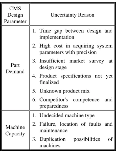
TABLE 1. Reasons for Considering Impreciseness in CMS Design Parameters.

CMS Design Parameter

Uncertainty Reason

Part Demand

1. Time gap between design and implementation

2. High cost in acquiring system parameters with precision

3. Insufficient market survey at design stage

4. Product specifications not yet finalized

5. Unknown product mix

6. Competitor's competence and preparedness

Machine Capacity

1. Undecided machine type

2. Failure, location of faults and maintenance

3. Duplication possibilities of machines

Mathematical programming is widely used in modeling CMS problems. Kusiak [2] proposed a generalized p-median model in the presence of alternative routings. Song, et al [3] considered a formation problem of a predetermined number of cells to maximize the total number of parts produced in cells by using the quadratic assignment problem (QAP) formulation. The proposed solution was a combination of the branch-and-bound (B,B) method based on the Lagrangian relaxation and a heuristic method. In many practical cases, a product mix or demand level may vary under a multi-period planning horizon. A DCMS considers reconfiguration of cells in each period and brings flexibility to form machine cells and part families. Some investigations have been carried out in the field of CFPs under dynamic conditions by Vakharia, et al [4], Harhalaks, et al [5], Wilhelm, et al [6], and Askin, et al [7]. Chen [8] proposed a mixed-integer programming (MIP) model that minimizes the reconfiguration costs, machine's constant costs, and intracellular movements. Since the model is NP-Complete, the proposed decomposition of the model to some simple sub-problems. Balakrishnan, et al [9] also considered a two-step model for the generalized machine assignment problem and dynamic programming for the CFP with changeable part demands.

Tavakkoli-Moghaddam, et al [10] developed the model, which was first proposed by Chen [8], with additional assumptions such as: alternative process plan, sequence operation, machine capacity and machine replication with the aim of minimizing the sum of machine total costs and inter-cell movement cost simultaneously. Defersha, et al [11] proposed a comprehensive mathematical model for a DCMS based on tooling requirements of the parts, tooling available on the machines, dynamic cell configuration, alternative routings, lot splitting, sequence of operations, multiple units of identical machines, machine capacity, operation cost, parts' outsourcing cost, tool usage cost, setup cost, cell size limits, and machine adjacency constraints.

Short life cycle, high variation manufacturing, unpredictable demand, and short lead-time have pushed production systems to operate dynamically under unreliable conditions [8]. Besides, marketing development takes the uncertain nature of the

model parameters into consideration based on the fuzzy theory. Table 1 lists a number of reasons for considering uncertainty in CMS design parameters [12].

Safaei, et al [16] presented a mixed-integer programming model for a dynamic cell formation problem with fuzzy parameters, such as part demand and machine availability. They proposed a fuzzy programming approach to determine the optimal cell configuration in each period with the maximum degree of satisfying the fuzzy objective under the given constraints. Torabi, et al [17] presented a new multi-objective possibilistic mixed-integer linear programming model with some fuzzy parameters, such as market demands, cost/time coefficients and capacity levels. They converted this model to a multi-objective linear model solved by their new interactive fuzzy approach.

In addition, the CFP considers many different objectives in a real-world situation; however, none of the above researchers have considered a comprehensive DCFP with multiple objectives and uncertain parameters for real-world conditions, such as sub-contraction possibilities or alternative process routings. This paper proposes an extended MINLP model with some fuzzy parameters for the CFP considering three objectives:

1. Minimizing the dynamic system total cost 2. Minimizing the intracellular workload

variation;

3. Maximizing the decision maker's (DM) utility (or minimizing the production volume deviation from the admissible demand). The main constraints are the cell size limitation, machine capacity, machine capability of processing an operation, machine investment, and production volume.

The novelty of the proposed model is to form cells in each period with respect to real-world practical aspects, such as lot splitting and outsourcing of parts and cell reconfiguration possibilities simultaneously. This model also considers uncertain environment using appropriate fuzzy membership functions for some parameters (i.e. production volume and machine capacity) and tries to reduce the computational complexity through arranging the mathematical model as simple and regular as possible to obtain an admissible set of answers for the DM.

The rest of this paper is organized as follows. Detailed description of the proposed model is described in Section 2. Section 3 discusses different approaches to multi-objective problems.

A numerical example and the computational results are reported in Section 4. Discussion and conclusion are presented in Section 5.

2. PROBLEM FORMULATION

In this section, we present a novel, multi-objective dynamic CFP with fuzzy parameters. The considered manufacturing system consists of several parts that required a number of operations on different machines with limited capacities according to a given sequence and for a number of time periods. Each machine can process different operations based on the tooling available and can be considered as alternative route for part processing. The demand for each part type per period is a piece-wise fuzzy number. Also, the uncertain capacity for each machine type is given as a triangular fuzzy membership function. The processing time for all operations on each machine type is known and each part has multiple process plans to be processed under. Machine maintenance cost is known and constant throughout the whole planning horizon, while it is independent from the assigned workload. The operation cost for each machine type per hour is known and varies with the workload assigned to that machine. Due to the dynamic reconfiguration of the cell in each period, the machine relocation from one cell to another is performed at the beginning of each period and with zero time duration. The relocation cost of any machine is independent from the existed primary place and its value is given.

Figure 1. Membership function for a fuzzy demand of part p in period t.

u m

C

m m

C

l m

C

α

( )

Cm

μ

m

C

α m

C

1

0

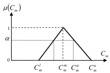
Figure 2. Membership function for a fuzzy capacity of

machine type m.

The workload assigned to machines of each cell is balanced within cells based on the time spent on processing of each part operation. The extra inventory between periods is zero; delayed order is forbidden and total demand in each period must be supplied in the same period. The setup time and the money time value are not considered. The time of machine installation is zero and machine breakdown is not considered.

In this paper, the problem considers the following attributes:

• Dynamic cell configuration in each period.

• Uncertain part-type demand. • Unreliable machine capacity.

• Flow flexibility (multiple process plan). • Route flexibility (alternative routing). • Lot splitting.

• Operation sequencing.

• Outsourcing a portion of demand.

• Machine relocation and cell

reconfiguration.

• Machine duplication in order to cover capacity limitations.

• Inter-cell movements of parts in batches of different sizes and handling costs per part-type.

• Intra-cell workload balance between machines.

• Cell size and number limitations.

The intervals for possible values of fuzzy parameters are specified by the user as

⎣

a

l

,

a

u

⎦

implicating a piece-wise membership function (see Figures 1 and 2). In general, piece-wise membership functions can be divided into two main intervals. The first interval represents “risk free” values in the sense that a solution should almost be implemental and realistic. On the other hand, the second interval represents “full risk” values that mean parameter values that are most certainly unrealistic, “impossible”, and the solution obtained by these values is not implemental. While moving from “risk free” toward “full risk” values, it is moved from solutions with a high degree to a low degree for implementation [18].

2.1. Notations

The notations of the proposed

model are described as follows:

p

: Part types;

p

=

1

,

2

,

K

,

P

j

: Operations required by part

p

;

p

J

j

=

1

,

2

,

K

,

m: Machine types;

j

=

1

,

2

,

K

,

J

_p

c: Manufacturing cells;

c

=

1

,

2

,

K

,

C

t

: Time types;

t

=

1

,

2

,

K

,

T

P

: Number of part types.

p

J

: Number of operations for part

p

.

M

: Number of machine types.

C: Maximum number of cells that can be formed.

T

: Number of manufacturing periods.

)

(

~

t

(

)

⎪ ⎪ ⎩ ⎪ ⎪ ⎨ ⎧

≥

< <

− −

≤

=

) ( ) ( 1

) ( ) ( ) ( ) ( ) (

) ( ) (

) ( ) ( 0

) (

t D t D

t D t D t D t D t D

t D t D

t D t D

t D

u p p

u p p

l p l

p u

p l p p

l p p

p μ

(1) From the point of the DM, the demand of part

p

in period

t

should be presumably equal and greater than Du_p(t). In other words, Du_p(t) indicates a desirable level for part demand. Therefore, the interval

(

Du_p(t),∞

)

presents a “risk-free” value-interval and

(

Dl_p(t),Du_p(t)

)

presents a “risk-full” value-interval for the decision maker. In the proposed model, there is a trade-off between maximizing the decision maker’s utility and minimizing the sum of traditional costs of the CFP. Thus, interval

[

Du_p(t),∞

)

is not considered in our model, because the production volume within this interval causes simultaneous increasing operation costs while the decision maker’s utility remains constant.

C~_m: Fuzzy capacity of machine m in terms of a triangular fuzzy number, as shown in Figure 2.

( )

0

Otherwise

l

l m

m m

m m m

m l

m m

u

m u

m m

m u m m m m

m m

C

C

C

C

C

C

C

C

C

C

C

C

C

C

C

μ

⎧

−

≤

≤

⎪

−

⎪

⎪

−

⎪

=

⎨

≤

<

−

⎪

⎪

⎪

⎪⎩

(2)

Equation 2 ensures that the capacity of each machine type m is supposed to be almost equal to

m m

C

. However, by considering unplanned failure to the machines or implementation of an accurate productive maintenance (PM) plan, this target may vary between

(

C

_ml

,

C

_mu

)

according to the specified membership function.

α

Cut-level. This parameter is

determined by the DM and used to

convert the fuzzy proposed model into a crisp parametric model. The

α

-level cut concept [20] limits the range of demand for part

p

in period

t

and capacity of machine type m according to the DM's preferences. For any

α

value, we have an optimal solution; so the solution with

α

grade of membership is actually fuzzy [21].

p

B

Batch size for inter-cell material movements for processing two consecutive operations of part type

p

.

p

V

Inter-cell material movement cost for each batch of part type

p

.

p

U

Subcontracting cost for each batch of part type

p

.

m

M

Maintenance cost of machine type m (constant).

m

O

Operating cost of machine type m per hour (variable).

jpm

h

Time required performing operation

j

of part type

p

on machine type

m(constant).

⎪ ⎩ ⎪ ⎨ ⎧

= =

) (

otherwise

0

type machine on

done be can part type of

operation if

1

0 h

m

p j

β

jpm jpm

m

r

Relocation cost of machine type m.

UB Upper bound for the cell size.

)

(

t

P

_m Purchasing cost of machine type m in period

t

.

)

(

t

Y

_m Maximum allowed number of machine type m to procure in period

t

.

)

(

t

w

_jpmc Workload on machine type m in cell

cdue to performing operation

j

of part type

p

in period

t

.

)

(

t

2.2. Decision Variables

)

(

t

N

_mc Number of machine type m in cell c in period

t

.

)

(

t

n

_mc+

Number of increased machine type m to cell c in period

t

.

)

(

t

n

_mc− Number of decreased machine type

m from cell c in period

t

.

)

(

~

t

Q

_p Production volume of part type

p

in period

t

.

)

(

t

jpmc

ε

The proportion of the total demand of part type

p

with operation

j

to perform by machine type m in cell c during period

t

.

)

(

t

p

δ

The proportion of the total demand of part type

p

to be subcontracted in period

t

.

⎪ ⎩ ⎪ ⎨ ⎧ = otherwise 0 period during cell in done be can part type of operation if 1 t c p j ) t ( Z_jpc

2.3. Mathematical Model

Based on the above

definitions, the proposed model for the CFP under dynamic and fuzzy conditions is illustrated as follows:

(

)

(

)

∑ ∑

∑

∑

∑∑ ∑

∑∑

∑ ∑ ∑

∑∑

∑∑ ∑∑∑

∑ ∑∑

= = = = = = = − + = = − = = = + = = = = = = = = = = ⎪⎭ ⎪ ⎬ ⎫ ⎪⎩ ⎪ ⎨ ⎧ ⎟ ⎟ ⎠ ⎞ ⎜ ⎜ ⎝ ⎛ − − + + + δ + ε − ε × ⎥ ⎥ ⎥ ⎤ ⎢ ⎢ ⎢ ⎡ + ε + = T t M m C c mc C c mc m m T t C c M m mc mc T t P p p p p J j C c M

m (j )pmc jpmc

T t p P p p p T t C c M m P p J j m jpm jpmc p T t M m C c m mc ) t ( N ) t ( N , max ). t ( P r . ) t ( n ) t ( n U ). t ( ). t ( Q~ ) t ( ) t ( V . B ) t ( Q~ o . h ). t ( ). t ( Q~ M ). t ( N Z min p p

2 1 1 1

1 1 1

1 1

1

1 1 1

1

1 1

1 1 1 1 1

1 1 1

1 1 0 2 1 2 1

(

)

∑∑∑∑∑

∑∑

= = = = = = =

−

=

−

=

T t M m C c P p J j jpc jpmc T t P p p u p p

t

w

t

w

Z

t

Q

t

D

Z

1 1 1 1 1

3 1 1 2

)

(

)

(

min

)

(

~

)

(

min

(3) s.t. t c m p j t _jpm

jpmc( )≤

β

∀ , , , ,

ε

(4)

t c m C t N h t t

Q _{mc m}

P p J j jpm jpmc p p , , ~ ). ( ). ( ). ( ~ 1 1 ∀ ≤

∑ ∑

= = ε (5) t c UB t N M m

mc( ) ,

1 ∀ ≤

∑

= (6) 1 , , ) ( ) ( ) ( ) 1

(t − +n+ t −n− t =N t ∀m c t >

Nmc mc mc mc

(7)

(

n t n t

)

Y_m t m t

C

c

mc

mc( ) ( ) ( ) ,

1 ∀ ≤ −

∑

= − + (8) t c p j t Z t M m jpc

jpmc( ) ( ) , , ,

1

∀ ≤

∑

=

ε (9)

∑∑

= = ∀ − = C c p M m

jpmc t t j p t

1 1 , , ) ( 1 ) (

δ

ε

(10)

t p t D t Q u p

p( )≤ ( ) ∀ , (11)

(

h Q t t

)

C j p m c t

t

w_jpmc()= _jpm.~_p( ).ε_jpmc( ) ~_m ∀ , , , ,

(12) t c p j t N t N t w t w M m mc M m mc jpmc

jpc() (). () () , , ,

1 1 ∀ ⎟ ⎠ ⎞ ⎜ ⎝ ⎛ ⎟ ⎠ ⎞ ⎜ ⎝ ⎛ =

∑

∑

= = (13) t , p ) t (

p ≤ ∀

δ

≤ 1

0 (14)

{ }

, j,p,c,t

) t (

Zjpc ∈ 01 ∀ (15)

( ), ( ), ( ), ( ) 0

mc mc mc p

N t n+ t n− t Q t_{% ≥}

The multi-objective function given in Equation 3 is a mixed-integer nonlinear equation consisting of three sub-functions. The first function (Z1) minimizes the total sum of machine maintenance costs (fixed), machine operating costs (variable), inter-cell material handling costs, machine relocation costs, operation outsourcing costs, and machine purchase costs. The first term of this equation is obtained by the product of the number of machine type m in cell c in period t and their associated constant costs. The second term is the sum of the product of the operational time that each machine needs to process the allocated quantity of parts and their associated variable costs. The third term is obtained by summing the product of the number of inter-cell transfers in batches and the unit batch inter-cell movement cost. The operation sequence directly affect the intercellular movements; i.e. if two consecutive operations must be processed by two machines in two different cells, then an unit inter-cell movement cost incurres. The forth term is the cost for sub-contracting parts based on their quantities. The fifth term is the sum of the number of products relocated (added or removed) machines and their associated cost. The sixth term is the machine procurement cost. If the total number of machines in a period is less than its previous period, this cost will not be considered.

The second and third functions (i.e., Z₂,

Z

3), are to overcome the deviation of the desired production volume and average intra-cell workload, respectively. Z₂ tries to minimize the deviation of the production volume from the admissible demand for all parts and in the whole planning horizon. It can be also considered equivalent to “

max

α

” in the fuzzy theory. The last objective function also minimizes the deviation of each machine type workload from the cell average, in order to balance the intracellular workload due to processing parts.

Equation 4 guarantees that each part of operation is assigned to a machine, which has the required tools for processing the job. Equation 5 ensures that machine capacity is not exceeded and can satisfy the demand. Moreover, this constraint determines the desired number of each machine type in each cell. Equation 6 specifies the upper bound of the cell size. It is obvious that lower sized

cells are more desirable. Equation 7 ensures that the number of machines in the current period is equal to the number of machines in the previous period, plus the number of machines being moved in, is deducted from the number of machines being moved out. In other words, this constraint acts like history for the problems. Equation 8 limits the maximum number of machines to be procured at the beginning of each period. Equation 9 ensures that a portion of operation j of part p can be done in cell c, if and only if the aforesaid cell is active in the period t. Equation 10 ensures that if a part is not subcontracted, the processing of each operation of this part must be assigned to a machine. Equation 11 determines upper bounds in form of the maximum demand for production volume related to each part in each period. Equations 12 and 13 identify the workload for each machine type in each cell and the average intra-cell workload, respectively, based on performing each part operation in every period. The values of

)

(

t

p

δ

are limited within [0,1] given by Equations 14 to 16.

2.4. Selection of Objectives

Though, there are several important objectives associated with the CF problem, it is very difficult to consider all objectives in a particular formulation. Ideally, it is preferred that a whole family of parts to be processed in one machine cell. However in typical industrial applications, it is difficult to accomplish, and hence, most studies have focused on minimizing inter-cell moves [22].

increased as expected results. Therefore, all these objectives have been proposed as cost centers in an integrated objective function in order to overcome the inherent conflict.

On the other hand, minimizing the tolerance between real and desirable production volume is necessary due to the fuzzy nature of the proposed model. Actually, the aim of this term is to maximize the decision maker's utility.

As the third independent objective, minimizing cell load variation, which is calculated as the difference between the workload on the machine and the average load on the cell, aids a smooth flow of materials inside each cell leading to the minimization of WIP within each cell [23].

2.5. Model Defuzzification

Since some parameters in form of variables and resources are uncertain and showed as fuzzy numbers, the proposed non-symmetric fuzzy model is converted into a crisp one by applying the

α

-cut concept according to the Verdegay's approach [24]. It means that the minimum preference level determined by the DM is equal to

α

. Therefore, we substitute the fuzzy demand for part p (

Q

~

_p) and fuzzy capacity of machine type m, by crisp parameters, named

Q

_p and

m

C

respectively, through defining appropriate

α

-cut constraints (see Equations 17 to 19):

(

D_p(t)

)

≥α ∀p,t

μ (17)

( )

C_m ≥α ∀m

μ (18)

1

0≤α≤ (19)

Membership functions of Equations 1 and 2 are substituted and then the following constraints are added to the primary model, which limit the production volume and machine capacity and indicate the confidence level of the DM.

(

)

D t p t

t D t

Q l

p u

p

p( )≥α. ()+ 1−α . () ∀ , (20)

m C ) C C ( C C ) C C

( _mm− _ml + _ml ≤ _m≤α _mm− _mu + _mu ∀

α (21)

2.6. Model Linearization

Since the objective function and some of the given constraints are

nonlinear due to maximum, absolute, and variables multiplication functions, we propose the linearization procedures below:

2.6.1. Linearizing the absolute function

The third term in the objective function can be linearized by introducing two non-negative variables

τ

_jpc+ (t) and

τ

_jpc− (t) and a binary variable

σ

_jpc

(

t

)

.

So, the term

∑

M₌

(

₊ −

)

m 1

ε

(j 1)pmc(t)

ε

jpmc(t) is

replaced by

τ

_jpc+ (t)+

τ

_jpc− (t) through adding Equation 22 [11].

(

)

{ }

( 1)

1 1

( ) ( ) ( ) ( ) , , ,

( ) . ( ) , , ,

( ) . 1 ( ) , , , (18) ( ) 0,1 , , ,

M M

j pmc jpmc jpc jpc

m m

jpc jpc

jpc jpc

jpc

t t t t j p c t

t M t j p c t

t M t j p c t t j p c t

ε ε τ τ

τ σ

τ σ

σ

+ − +

= =

+

−

− = − ∀

≤ ∀

≤ − ∀

∈ ∀

∑

∑

(22) Consider M as a large positive number. The same

procedure is used for linearization of the last term of the objective function.

2.6.2. Linearizing the maximum function

The sixth term in the objective function can be also linearized introducing two non-negative variables

)

(

t

k

_m+

and

k

_m−

(

t

)

and a binary variable

θ

_m

(

t

)

. So, the term max

{

0,

∑

C_c=1

(

Nmc(t)−Nmc(t−1)

)

}

is

replaced by

k

_m+

(

t

)

through adding Equation 23 [11].

(

)

{ }

m

t

t

t

m

t

M

t

k

t

m

t

M

t

k

t

m

t

k

t

k

t

N

t

N

m

m m

m m

m m

C

c mc C

c mc

,

1

,

0

)

(

,

)

(

1

.

)

(

,

)

(

.

)

(

1

,

)

(

)

(

)

1

(

)

(

1 1

∀

∈

∀

−

≤

∀

≤

>

∀

−

=

−

−

− +

− +

=

=

∑

∑

θ

θ

θ

(23) 2.6.3. Linearizing the decision variables

Equations 25 to 28, respectively, as follows:

t p t

S t t Q

t c m p j t

X t t

Q

p p

p

jpmc jpmc

p

, )

( ) ( ). (

, , , , )

( )

( ). (

∀ =

∀ =

δ

ε

(24)

t

c

m

p

j

M

t

X

_jpmc

(

)

_jpm

,

,

,

,

:

)

4

(

≤

β

∀

(25)

h c p j t

MZ t X

M

m

jpc

jpmc() () , , ,

: ) 9 (

1

∀ ≤

∑

=

(26)

∑∑

= =

∀ −

= C

c p p

M

m jpmc

t p j t

S t Q t X

1 1

, , ) ( ) ( ) ( :

) 10

( (27)

t

p

t

Q

t

S

_p

(

)

_p

(

)

,

0

:

)

14

(

≤

≤

∀

(28)

3. MULTI-OBJECTIVE SOLUTIONS

The solution approaches to the multi-objective cell formation (MOCF) problem may be classified to four broad categories: 1. Weighting method; 2. goal programming; 3. heuristic methods; and 4. search methods [23].

In the first approach, which is applied to this paper, a set of objectives are considered and is converted into a single objective by the weighted sum of individual objectives. Although this approach offers only a compromise solution whose non-dominance is not guaranteed, it provides the flexibility of assigning different weights to different objectives based on DM's requirements, which is a great advantage in MODM and fuzzy environment [25].

The second approach attempts to minimize a set of deviations from the prescribed multiple goals, which are considered simultaneously; however, these goals are satisfied according to their priority levels. The main drawback of the approach is the ability to provide only a single non-dominated solution, so the model has to be solved again with a different set of parameters in case of DM's dissatisfaction [26].

The third and forth approaches are kinds of heuristic and meta-heuristic methods, such as simulated annealing (SA), tabu search (TS), and genetic algorithm (GA), that are very effective in

solving complex multi-objective optimization problems. However, these methods may not find optimal solutions, and the associated results are somehow dependent on the chosen values of search parameters [23]. These methods are not addressed in this paper; however, they are recommended for future studies to prevail over computational complexity of the novel proposed model.

Since the proposed triple objective model consists of a comprehensive cost function and two deviation minimization objectives, we use a type of weighting method and consider two monetary penalty parameters, named

λ

₁ and

λ

₂, to overcome the deviation of the desired production volume and average intra-cell workload, respectively.

1

λ

Unit penalty of the production volume deviation from the admissible demand (Du_p(t)).

2

λ

Unit penalty of each machine workload deviation from the average intra-cell workload (Du_p(t)).

Thus, the multi-objective function, which has been proposed by Equation 3, is converted to an integrated cost-based single-objective one (see Equation 29).

3 2 2 1

1 .Z .Z

Z Z

min = +λ +λ (29)

Besides, the penalties are defined by the DM in order to provide required flexibility and take the real-world conditions into consideration. However, the prescribed range to both the parameters can be obtained by analyzing multiple examples with different values.

4. COMPUTATIONAL RESULTS

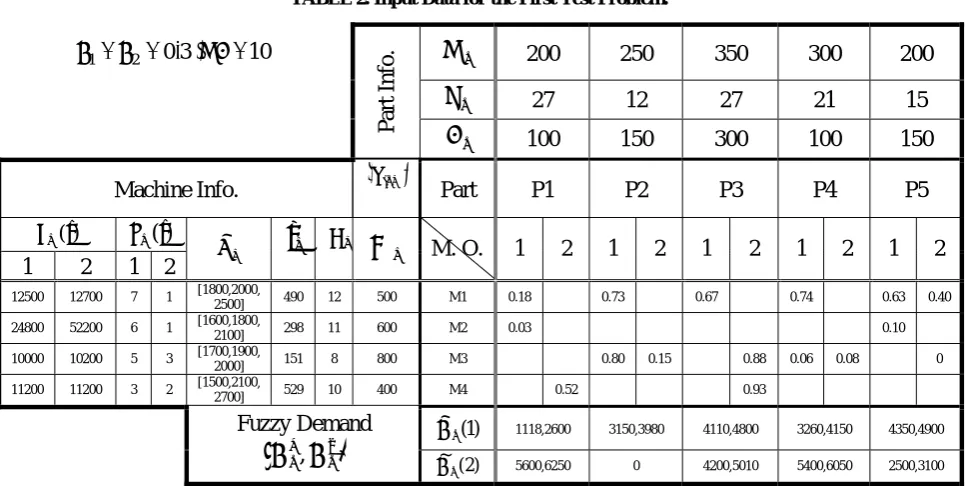
TABLE 2. Input Data for the First Test Problem.

200 300

350 250

200

p

U

10

3 0

2

1=λ = =

λ . ,UB

15 21

27 12

27

p

V

150 100

300 150

100

p

B

Part Info.

P5 P4

P3 P2

P1 Part

( )

hjpm

Machine Info. ) (t

Y_m

) (t P_m

2 1 2 1 2 1 2 1 2 1 M. O.

m

M

m

O

m

r

m

C~

2 1 2 1

0.40 0.63 0.74

0.67 0.73

0.18 M1 500

12 490 [1800,2000,

2500] 1

7 12700 12500

0.10 0.03

M2 600

11 298 [1600,1800,

2100] 1

6 52200 24800

0 0.08

0.06 0.88 0.15

0.80 M3

800 8 151 [1700,1900,

2000] 3

5 10200 10000

0.93 0.52

M4 400

10 529 [1500,2100,

2700] 2

3 11200 11200

4350,4900 3260,4150

4110,4800 3150,3980

1118,2600

) 1 ( ~

p

D

2500,3100 5400,6050

4200,5010 0

5600,6250

) 2 ( ~

p

D Fuzzy Demand

[

u

]

p l

p D

D ,

GHz Laptop with 2.00 Gb RAM. Then, the associated computational results are reported. The first example is a small-sized problem and considers M = 4, P = 5, and C = 2 to produce parts with fuzzy demands in two periods, and each product must be processed under 2 operations. In addition, some of the operations can be done on 2 alternative machines with different processing times.

The input parameters are shown in Table 2. The maximum cell size (number of machines in each cell) is set to 10 and the deviation penalties, λ1 and λ1, are supposed equivalent to 0.3 monetary units. The uncertainty parameter is set to 0.8 to provide a high imprecision utility for the DM. In addition, the software run time is limited to one hour (i.e. 3600 seconds).

The NP-hardness of standard CFP models has been explicitly discussed in some previous studies [10,27]. Furthermore, compromising a number of fuzzy parameters in the proposed model contributes to increase the problem NP-hardness. Therefore, the proposed model cannot be solved optimally within a reasonable amount of time for real-world instances, because of its nonlinear and NP-hard nature.

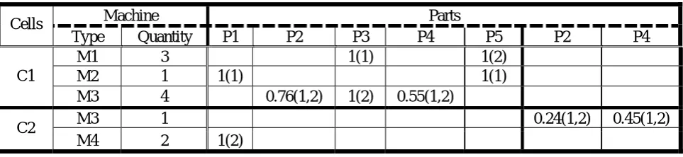
The cells generated in each period and the parts

assigned to the various cells are given in Tables 3 and 4, respectively. The values in the table intersections show the value of εjpmc(t). The

operation sequence can be obtained from the parentheses in these tables. The best feasible objective value found so far is 292558 monetary units while the objective bound is 290699.

Thus, the optimal objective value of the given test problem must be in [Obj Bound, Best Obj] = [290699,292558] interval, with a gap of 0.64 %, according to the Lingo software documents. As shown in Table 3, in the first period, Part 1 must move between cells 1 and 2 to do consecutive operations resulting in an inter-cell transportation cost. So, this part is considered as “exceptional element”. Part types 2 and 4 split between two cells due to alternative process plans.

TABLE 3. Cell Formation for Period 1 of the First Test Problem.

Parts Machine

P4 P2

P5 P4

P3 P2

P1 Quantity Type

Cells

1(2) 1(1)

3 M1

1(1) 1(1)

1 M2

0.55(1,2) 1(2)

0.76(1,2) 4

M3 C1

0.45(1,2) 0.24(1,2)

1 M3

1(2) 2

M4 C2

TABLE 4. Cell Formation for Period 2 of the First Test Problem.

Parts Machine

Cells

P4 P3

P2 P5

P4 P3

P2 P1

Quantity Type

1(2) 1(1)

0.5(1) 3

M1

1(1) 1 (1)

1 M2

0.73(1,2) 0.6(2)

0.25(1,2) 2

M3 C1

0.27(1,2) 0.4(2)

0.25(1) 0.75 (2) 1

M3

1(2) 2

M4 C2

TABLE 5. Values of the Decision Variables for the First Test Problem.

M1 M2 M3 M4

Machine Capacity 2100 1860 1920 2220

Periods P1 P2 P3 P4 P5

T1 2304 3814 4662 3972 4790

Part Quantity

T2 6120 0 4848 5920 2980

each machine is balanced in each cell of the given example and increases the efficiency of the cell formation.

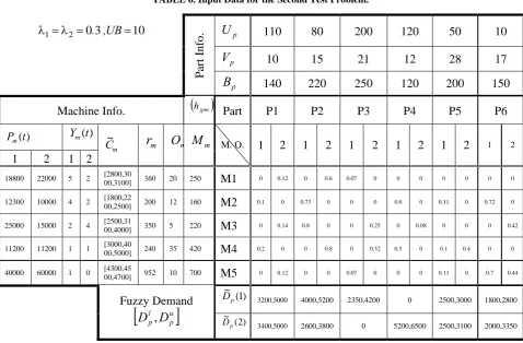
The second example is a medium-sized problem considering M = 5, P = 6 and C = 3 to produce parts with fuzzy demands in two periods, in which each product must be processed under 2 operations and some operations can be done on 2 or 3 alternative machines with different

TABLE 6. Input Data for the Second Test Problem.

10 50

120 200

80 110

p

U

10

3 0

2

1=λ = =

λ . ,UB

17 28

12 21

15 10

p

V

150 200

120 250

220 140

p

B

Part Info.

P6 P5

P4 P3

P2 P1

Part

( )

hjpm

Machine Info. ) (t

Y_m

) (t P_m

2 1

2 1 2 1 2 1 2 1 2 1 M. O.

m

M

m

O

m

r

m

C~

2 1 2 1

0 0 0 0 0 0 0 0.07 0.6 0 0.12 0

M1 250

20 360 [2800,30 00,3100] 2

5 22000 18800

0 0.72 0 0.11 0 0.6 0 0 0 0.73 0 0.1

M2 160

12 200 [1800,22 00,2500] 2

4 10000 12300

0.42 0 0 0 0.08 0 0.25 0 0 0.8 0.14 0

M3 220

5 350 [2500,31 00,4000] 4

2 15000 25000

0 0 0.4 0.1 0 0.5 0.52 0 0.8 0 0 0.2

M4 420

35 240 [3000,40 00,5000] 1

1 11200 11200

0.44 0.7 0 0.11 0 0 0 0.07 0 0 0.12 0

M5 700

10 952 [4300,45 00,4700] 0

1 60000 40000

1800,2800 2500,3000

0 2350,4200 4000,5200

3200,5000

) 1 ( ~

p

D

2000,3350 2500,3100

5200,6500 0

2600,3800

3400,5000

) 2 ( ~

p

D Fuzzy Demand

[

u

]

p l

p D

D ,

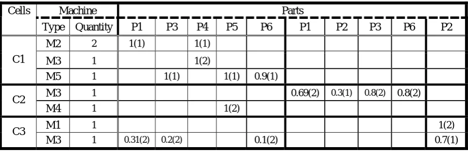
problem. The first cell is reconfigured in the second period by purchasing a unit of machine type 1. In addition, the part assigned to the three cells has noticeable changes during period alteration.

5. CONCLUSION

In this paper, we have proposed a new multi-objective dynamic cell formation model as a fuzzy parametric mixed-integer nonlinear programming to minimize dynamic manufacturing costs, maximize the decision maker's utility, and balance the intracellular workload simultaneously by integrating the objectives into a complex cost-based objective function. The main advantages of the proposed model are to form part families and machine cells simultaneously, determine the best processing route for each part type per period,

reconfigure cells between two consecutive periods if necessary, and specify the most suitable production quantity for each part.

TABLE 7. Cell Formation for Period 1 of the Second Test Problem.

Parts Machine

Cells

P2 P6

P3 P2

P1 P6

P5 P4 P3 P1

Quantity Type

1(1) 1(1)

2 M2

1(2) 1

M3

0.9(1) 1(1)

1(1) 1

M5 C1

0.8(2) 0.8(2)

0.3(1) 0.69(2)

1 M3

1(2) 1

M4 C2

1(2) 1

M1

0.7(1) 0.1(2)

0.2(2) 0.31(2)

1 M3

C3

TABLE 8. Cell Formation for Period 2 of the Second Test Problem.

Parts Machine

Cells

P4 P2

P6 P2

P1 P6

P5 P4 P3 P1 Quantity Type

1(1) 1

M1

1(1) 1(1)

2 M2

1(2) 1

M3

1(1) 1(1) 1

M5 C1

0.69(2) 0.68(1)

0.54(2) 0.17(2)

1 M3

1(2) 1

M4 C2

1(2) 1

M1

0.83(2) 0.32(1)

0.31(2) 0.45(2)

1 M3

C3

TABLE 9. Values of the Decision Variables for the Second Test Problem.

M1 M2 M3 M4 M5

Machine Capacity 3020 2260 3280 4200 4540

Periods P1 P2 P3 P4 P5 P6

T1 4640 4960 3830 0 2900 2600

Part Quantity

T2 4680 3560 0 6240 2980 3080

6. ACKNOWLEDGEMENT

This study was supported partially by the

7. REFERENCES

1. Rheault, M., Jocelyn, D. and Geoges, A., “Physically

Reconfigurable Virtual Cells: A Dynamic Model for a

Highly Dynamic Environment”, Computers and

Industrial Engineering, Vol. 29, (1995), 221-225.

2. Kusiak, A., “The Generalized Group Technology

Concept”, International Journal of Production

Research, Vol. 20, No. 2, (1987), 117-133.

3. Song, S. and Hitomi, K., “Integrating the Production

Planning and Cellular Layout for Flexible Cellular

Manufacturing”, Production Planning and Control,

Vol. 7, No. 6, (1996), 585-593.

4. Vakharia, A. J. and Kaku, B. K., “Redesigning a

Cellular Manufacturing System to Handle Long-Term Demand Changes: A Methodology and Investigation”, Decision Sciences, Vol. 24, No. 5, (1993), 909-929.

5. Harhalaks, G., Nagi, R. and Proth, J., “An Efficient

Heuristic in Manufacturing Cell Formation to Group

Technology Applications”, Int. Journal of Production

Research, Vol. 28, No. 1, (1990), 185-198.

6. Wilhelm, W., Chiou, C. and Chang, D., “Integrating

Design and Planning Considerations in Cellular

Manufacturing”, Annals of Operation Research, Vol.

77, No. 1, (1998), 97-107.

7. Askin, R. G., Selim, H. M. and Vakharia, A. J., “A

Methodology for Designing Flexible Cellular

Manufacturing Systems”, IIE Transactions, Vol. 29,

(1997), 599-610.

8. Chen, M., “A Mathematical Programming Model for

Systems Reconfiguration in a Dynamic Cell Formation

Condition”, Annals of Operations Research, Vol. 77,

No. 1, (1998), 109-128.

9. Balakrishnan, J. and Cheng, C. H., “Dynamic Cellular

Manufacturing under Multi-Period Planning Horizons”,

Journal of Manufacturing Technology Management,

Vol. 16, No. 5, (2005), 516-530.

10. Tavakkoli-Moghaddam, R., Aryanezhad, M. B., Safaei,

N. and Azaron, A., “Solving a Dynamic Cell Formation

Problem using Metaheuristics”, Applied Mathematics

and Computations, Vol. 170, No. 2, (2005a), 761-780.

11. Defersha, F. M. and Chen, M., “A Comprehensive

Mathematical Model for the Design of Cellular

Manufacturing System”, International Journal of

Production Economics, Vol. 103, (2006), 767-783.

12. Shankar, R. and Vrat, P., “Some Design Issues in

Cellular Manufacturing using the Fuzzy Programming

Approach”, International Journal of Production

Research, Vol. 37, No. 11, (1999), 2545-2563.

13. Seifoddini, H., “A Probabilistic Model for Machine Cell

Formation”, Journal of Manufacturing Systems, Vol.

9, No. 1, (1990), 69-75.

14. Tavakkoli-Moghaddam, R., Safaei, N. and Babakhani,

M., “Solving a Dynamic Cell Formation Problem with Machine Cost and Alternative Process Plan by Memetic

Algorithms”, Lecture Notes in Computer Science, Vol.

3777, (2005b), 213-227.

15. Tavakkoli-Moghaddam, R., Aryanezhad, M. B., Safaei,

N., Vasei, M. and Azaron, A., “A New Approach for the Cellular Manufacturing Problem in Fuzzy Dynamic

Conditions by a Genetic Algorithm”, Journal of

Intelligent and Fuzzy Systems, Vol. 18, No. 4, (2007), 363-376.

16. Safaei, N., Saidi-Mehrabad, M.,

Tavakkoli-Moghaddam, R. and Sassani, F., “A Fuzzy Programming Approach to a Cell Formation Problem

with Dynamic and Uncertain Conditions”, Fuzzy Sets

and Systems, Vol. 159, No. 2, (2008), 215-236.

17. Torabi, S. A. and Hassini, E., “An Interactive

Possibilistic Programming Approach for Multiple

Objective Supply Chain Master Planning”, Fuzzy Sets

and Systems, Vol. 159, No. 2, (2008), 193-214.

18. Arikan, F. and Gungor, Z., “A Parametric Model for

Cell Formation and Exceptional Elements' Problems

with Fuzzy Parameters”, Journal of Intelligent

Manufacturing, Vol. 16, (2005), 103- 114.

19. Tavakkoli-Moghaddam, R. and Safaei, N., “A

Generalized Dynamic Cell Formation Problem with

Fuzzy Demand and Unreliable Facilities”, Proceeding

of the 3rd International Conference on Group

Technology/Cellular Manufacturing, Groningen,

Netherlands, (2006), 349-356.

20. Tanaka, H., Okuda, T. and Asai, K., “On Fuzzy

Mathematical Programming”, Journal of Cybernetics,

Vol. 3, (1974), 37-46.

21. Lai, Y. J. and Hwang, C. L., “Fuzzy Mathematical

Programming: Methods and Applications”, Lecture Notes in Economics and Mathematical Systems, Springer-Verlag, Berlin Heidelberg, (1992).

22. Logendran, R., “Effect of the Identification of Key

Machines in the Cell Formation Problem of Cellular

Manufacturing Systems”, Computers and Industrial

Engineering, Vol. 20, No. 4, (1990), 439-449.

23. Agarwal, D., Sahu, S. and Ray, P. K., “Cell Formation

in Cellular Manufacturing: A Multi-Objective Genetic

Algorithm Approach”, Group Technology /Cellular

Manufacturing Conference, Groningen, Netherlands, (2006), 401-410.

24. Verdegay, J. L., “Fuzzy Mathematical Programming, in:

M. M. Gupta and E. Sanchez (Eds.)”, Fuzzy Information and Decision Processes, Publishing Company, Amsterdam, North-Holland, (1982), 231-237.

25. Venugopal, V. and Narendran, T. T., “A Genetic

Algorithm Approach to the Machine Component

Grouping Problem with Multiple Objectives”, Computers

and Industrial Engineering, Vol. 22, No. 4, (1992), 469-480.

26. Mansouri, S. A., Hussaini, S. M. M. and Newman, S. T.,

“A Review of the Modern Approaches to Multi-Criteria

Cell Design”, International Journal of Production

Research, Vol. 38, No. 5, (2000), 1201-1218.

27. Vin, E., Lit, P. and Delchambre, A., “A Multiple-Objective Grouping Genetic Algorithm for the Cell

Formation Problem with Alternative Routings”, J. of