THE ANALYSIS OF A BEAM UNDER MOVING LOADS
Department of Civil Engineering, Urmia University, Urmia, Iran e.mardani@urmia.ac.ir
*Corresponding Author
(Received: March 15, 2010 – Accepted in Revised Form: September 15, 2011)
doi:10.5829/idosi.ije.2011.24.03b.03
Abstract It is assumed that a beam made of material has a physical nonlinear behavior. This beam is analyzed under the moving concentrated and distributed continuous loads. The vibration equations of motion are derived from the Hamilton's Principle and Euler–Lagrange Equation. In this study, the amplitude of vibration, circular frequency, bending moment, stress and deflection of the beam has been calculated. At the state of concentrated moving load, the obtained analytic solution has been exemplified. The results of this study indicate that when the material of the beam is considered physically nonlinear, there is no critical velocity and the resonance phenomenon doesn’t happen.
Keywords:Moving Load, Hamilton Principle, Euler- Lagrange Equation, Duffing Equation, Resonance
1. INTRODUCTION
The study of dynamical effect of moving loads at highway and railroad bridges has a history of more than one and a half century. The collapse of Jester Bridge in England in 1847 encouraged both the theoretical and experimental studies. The catastrophe caused tremendous human losses and created a lot of excitement in civil engineering.
Presently, there are many structures made from materials which are not subject to the Hook’s law. Therefore, there is a great tendency to study stress and strain in elements of structures made of physical nonlinear material under various static and dynamic loads. In the linear theory, the property of material is not taken into consideration; however, all of relevant parameters are taken into consideration in the theory of nonlinear. Thus, the physical nonlinear theory
demonstrates an exact calculation method for the analysis of stress, strain, and other internal forces
in structural elements.
In order to represent all the possible states of the material by one mathematical law, the following algebraic function may be introduced:
2 3
This equation is not different from the general and.
f
Manzhaalovsky employed Empeher’s method and proposed the following two-term equations of the parabolic type on the basis of the tests carried out by Glushkov [1].
1 1 1
2 2 2 2
ﻩﺩﺮﺘﺴﮔﻭﻙﺮﺤﺘﻣ ﺰﮐﺮﻤﺘﻣ ﺭﺎﺑﺖﺤﺗ ﻲﻜﻳﺰﻴﻓ ﻲﻄﺧﺮﻴﻏﺭﺎﺘﻓﺭ ﺎﺑﺢﻟﺎﺼﻣ ﺯﺍ ﻩﺪﺷ ﻪﺘﺧﺎﺳ ﺮﻴﺗﻚﻳ ﻪﻛﺩﻮﺸﻴﻣ ﺽﺮﻓ
ﻩﺪﻴﮑﭼ
ﮋﻧﺍﺮﮔﻻ-ﺮﻠﻳﻭﺍﺕﻻﺩﺎﻌﻣﻭﻥﻮﺘﻠﻴﻣﺎﻫﻞﺻﺍﺯﺍﻩﺩﺎﻔﺘﺳﺍﺎﺑﻲﺷﺎﻌﺗﺭﺍﺖﻛﺮﺣﻞﻴﺴﻧﺍﺮﻔﻳﺩﺕﻻﺩﺎﻌﻣ .ﺩﻮﺷﻲﻣﺰﻴﻟﺎﻧﺁ ﮎﺮﺤﺘﻣﺖﺧﺍﻮﻨﻜﻳ ﺭﺩ .ﺩﻮﺷﻲﻣﻪﺒﺳﺎﺤﻣﺮﻴﺗﺰﻴﺧﻭﻲﺸﻤﺧﻥﺎﻤﻣ ,ﻲﻧﺍﺭﻭﺩﻲﻌﻴﺒﻃﺲﻧﺎﻛﺮﻓ ,ﻲﺷﺎﻌﺗﺭﺍﺖﻛﺮﺣﻪﻨﻣﺍﺩ ,ﻲﺳﺭﺮﻳﻦﻳﺍﺭﺩ .ﺪﻳﺁﻲﻣ ﺖﺳﺪﺑ
ﺮﻴﺗﺢﻟﺎﺼﻣ ﻲﺘﻗﻭﻪﻛﺖﺳﺍ ﻩﺪﺷﺺﺨﺸﻣ ﻪﺠﻴﺘﻧ ﺭﺩﻭﻩﺪﺷ ﻪﺋﺍﺭﺍﻱﺩﺪﻋ ﻝﺎﺜﻣ ﺕﺭﻮﺼﺑﻲﻠﻴﻠﺤﺗﻞﺣ ﻙﺮﺤﺘﻣ ﺰﻛﺮﻤﺘﻣﺭﺎﺑﺖﻟﺎﺣ
.ﺪﺘﻓﺍﻲﻤﻧﻕﺎﻔﺗﺍﺲﻧﺎﻧﻭﺯﺭﻩﺪﻳﺪﭘﻭﺩﺭﺍﺪﻧﺩﻮﺟﻭﻲﻧﺍﺮﺤﺑﺖﻋﺮﺳﺖﺳﺍﻲﻜﻳﺰﻴﻓﻲﻄﺧﺮﻴﻏﺭﺎﺘﻓﺭﻱﺍﺭﺍﺩ
E. Mardani*
(1)
(2)
(3) at small deformations
relationship between
1 2 3
2
where, 1, 2, 1 and 2 are empire elasticity.
Trinomial equations of the parabolic type were suggested for cast iron by Glushkov who proposed the use of a similar relationship for metal wire [1]:
3
2
b c (5)
In addition to exponential and power laws, hyperbolic relationships were suggested for brittle materials. Accordingly, as introduced the following function for cast iron:
(6)
Glushkov [1] has developed a theory for bars and discs made of brittle materials, employed the following hyperbolic laws:
1
Finally, the relationship between stress and strain, in the case of physical nonlinear, is presented by Kauderer [2]. As the equation proposed by Kauderer is comprehensive and expresses the relationship between the stress and strain in three dimensional states, we preferred to use the equation for the analysis of the physical nonlinear stress and strain
2 0 0 0
where, ij 0
stress:
(10)
K and G at small deformation are respectively volume contraction and shear elastic module. The relationship among K, E, and G is indicated through the following equation:
E (11)
K () is average stress function and l
t02 isshear stress function; it can be indicated through the following equation:
0 2 0 2 4
0 4 2 0 2 2
0
0 0 2
0 2 0 1 0
... 1
) (
... 1
) (
n n n
n n n
t l t
l t l t
l
K K
K
K
(12)
Researches have demonstrated that K () in
physical nonlinear material on an
deformation is close to the straight line (i.e., K ()
= 1). Also, the two first sentences of the shear stress function are enough.
2 0 2 2
0
2
l
is the physical nonlinear coefficient.As the Eq. (9) indicates, stress components of Z, y, and xy are created. The simplification of
the equation suggests that the stress components are too small in comparison with the Z. These
new components of the stress have less impact on the frequency of vibration and on the other parameters during the vibration of the beam. As a result, the following equation is obtained from the Eq. (9) at a two dimensional surface:
)
3 3 3
2
(14)
The purpose of this paper was the analysis of a beam made of physical nonlinear material under the moving concentrated and distributed continuous loads, which was discussed through examples analytically.
2. THEORY
2.1. Analytical solution for moving concentrated load To study the effect of moving load on the
prismatic beam, first, we are discussing moving concentrated load. Thus, it is assumed that the load P moves along the beam (Fig. 1).
(9) (8) (7)
(13) average relative
E
ij ij 0 ij
K( ) l(t )
3K 2G
i , j = 1 , 2 , 3
3
9KG
0 b
is Croneker symbols, and is average
( δ )
1
AB
x y z
5KG
27 G
E( l
Z Z Z
2 E
l(t ) 1 l t
Figure 1. Schematic view of a prismatic beam under moving load
To consider the effect of external moving load, it is assumed an equivalent distributed load which depends on z and t as follows [3]:
1 2 sin sin ) , ( k L z k L a k L P t z
q
(15)where,
L z k z
p( )sin , (k = 1,2,3,…) is the head vibration mode of the beam.
Therefore, the potential and kinetic energy of the system will be as follows [4]:
L dz
z w J G E l z w E J 0 4 2 2 1 3 4 2 2 2 2 0 54 1 2
1 (16)
L dz
t w F Ki 0 2 2 1
(17) Also, the work of the external moving load will be as follows [5]:
L L dz t z w L z k L a k L P A dz t z w t z q A 0 0 , sin sin 2 , . ,
(18)The Hamilton's Principle for this beam will be
dt dz t w F t z w L a k L a k L P z w J G E l z w E J dt Ki A H k t t t t L . 2 1 , sin sin 2 54 1 2 1 2 1 4 2 2 1 3 4 2 2 1 2 1 0 2 2 2 0
(19)where, J
y dxdy J
y4dxdy1 2 0 , Considering: t L z 0 ,
, which
,
varies respectively from 0 to and 0 to 2.where, 0 is circular frequency vibration of the system in linear case and expressing in Hamilton principle (19), the following equations are obtained: .
d d t w F w k k L P w L J G E L E J L H k w . 2 1 , . sin sin 2 54 1 2 1 2 2 0 1 0 4 2 2 8 8 1 3 4 2 2 2 4 4 0 0
(20)We assumed that the deformation of the beam would be found from the following expression [7]:
p
q w , (21) where, p
and q
are coordinate and generalized functions respectively.By substitution of expression (21) in expression (20), we obtain the following expressions:
d d q p F q p k L vt k L P q p L J G E l q p L E J L H k . 2 1 sin sin 2 54 1 2 1 2 2 2 0 1 4 4 8 8 1 3 4 2 2 2 20 0 4
4 0 0
(22)The following expression is derived from the calculations indicated above in Eq. (22) [8]:
2 0 0 2 0 2 2 0 4 2 0 Nd L d q d q c bq aq L H (23)P
a=vt
Z
L
P
[6]:
L vt k L P d d p F c d p L J G E l b d p L E J a sin 2 1 54 1 2 1 0 2 0 4 8 8 1 3 4 2 0 2 4 4 0
(24)For Integral (23), Euler equation gives [9]:
0 4 2 2 4 2 2 2 0 3 2 0 3 2 0 2 0 d bq aq q c d bq aq q N q c q c q N q N (25) L vt k L P d q a b aq qc 2 1 2 sin
2 2 2
0
(26)
By substitution of
0 ,
t
L k
into Eq. (26) we’ll have:
2 1 2 2 sin
0 q d
a b q c a
q
(27)
where, cL P d 2 , 0
By substitution of q d X
2 0
into Eq. (27), X is dynamic coefficient. We will have:
1 2
sin X eX
X (28)
where, 4 0 2 2 d a b
e (29)
To solve the Duffing Eq. (28), we follow the following procedure [10]:
5 sin 3 sin sin sin 5 3 , 5 , 3 , 1 1 X X X X X nn (30)
If we substitute the expression (30) into 28, and compare the similar coefficients of sinn, we will get a lot of cubic nonlinear algebraic equations. To our knowledge, there is no exact solution for these equations. Thus, we employed an approximated method. For this purpose, we applied three constraints Eq. (30) and we assumed that Xn
>> Xn+1: therefore, in this case, we will have the
following system of nonlinear equations:
0 2 3 2 3 4 3 4 3 4 3 25 1 0 4 3 2 3 2 3 2 3 4 3 11 1 9 1 1 2 3 4 3 2 3 4 3 2 3 4 3 1 5 2 1 5 2 3 2 3 1 3 2 1 3 5 5 2 5 2 1 2 5 3 3 2 1 5 3 1 3 3 3 1 3 2 2 5 1 5 2 3 2 3 1 3 2 1 5 3 1 3 1 1 2 X X X X X X X X X e X X X X X X X X X X X X e X X X X X X X X X X X X X e X (31)With solving of Eq. (31) by the method of Zeidel, we will have [11]:
14 3
1 3
1 1
2
X eX
25 1
4 3 1 9 4 2 3 1 3 1 5 2 3 1 3 X X X ex X x e
X (32)
When the load is out of the beam, Eq. (27) will be as below in which the system will have free vibration. 0 2 1 2 2 2 2 q a b q c a d dq
(33)
Finally, by solving Eq. (33), we found the period of vibration:
k Q a b c a T 2 14 (34)
Consequently, the circular frequency is as follows:
K Q a b c a 1 1 22
(35)
where,
2 4 sin6
256 25 sin 64
9 sin 4 1 1 2 K
is the circular frequency of vibration, Q is amplitude of vibration, and k () is a second order elliptic integral. As the above equation indicates,
2 Q a
b has a minus sign, which decreases the in comparison with 0 (as it was indicated in 35).
Based on the equations expressed above, the explanation of the analysis of deflection, bending stress, and bending moment are as follows.
Deflection: Deflection is obtained from the Eq.
(21).
d p EJ
Pl d
and t V a
l a X l
a X l
a X l
a n X
l a n X l
z d t z W
n n
n n
2 3
0 3
2
5 3
1 5
, 3 , 1
5 , 3 , 1 2
" ,
5 sin 3
sin sin
sin
sin sin
) , (
(36)
As it will be indicated in the tables below, the coefficients X3and X5are too small and neglected.
l a l
z X d t z
W
sin sin
) ,
( 2 1 (37)
Bending Stress: Bending Stress is calculated by
using Eq. (14) and 2 2
z w y
Z
, which is called KIRHOF principle.
3
2 2
3 3
2 2 2
27 2
z w y G E l z
w y E
Z
(38)
Bending Moment: Bending Moment in every
section of the beam is designed by the following equations:
2 2
0 1 3 3 2 2 2 0
2 2 3 3 2 2 2
. 27
2 1
27 2
z w J J G E l z
w Ej M
dy dx z
w y G E l z
w y E dy dx y
M Z (39)
The expression 2 2
z w
equals the following equation:
l a l
z l
d z
w
. 2 sin sin 2
2 0 2 2
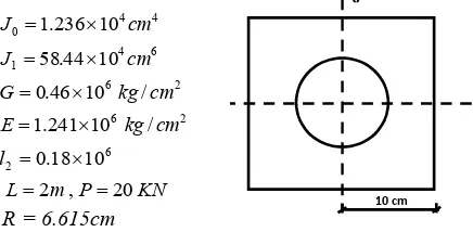
Now the obtained analytic solutions are being applied to the following example. It has been assumed that the material of the beam is copper (Fig. 2).
KN P
m L l
cm kg E
cm kg G
cm J
cm J
20 , 2
10 18 . 0
/ 10 241 . 1
/ 10 46 . 0
10 44 . 58
10 236 . 1
6 2
2 6
2 6
6 4 1
4 4 0
R = 6.615cm
Figure 2.Section of beam
Then vibration amplitudes are determined and are shown in Table 1.
TABLE 1. Dimensionless vibration amplitudes
2
1 X1 X3 X5
1
1 2
1 3
0.0 -40.2 -39.83 1.00 -16.11 -22.04 -3
-4
-6 -11
Based on Table (1) the diagram of resonance
Figure 3. Resonance Curve
10 cm
Y
2 is indicated in Fig. 3.
X X X
0.84 -21.07 10.54 0.1902 -1.31 10
1 -11.73 0.041 -1.01 10
2 1.00 3.69 10 -1.63 10
|X|
Deflection, stress, and bending moment in the section of the beam are calculated by using equations (36), (37), and (38) for 21 and za, which are indicated in Tables 2 and 3.
moment at the point of load a
8
l
4
l
8 3l
2
l
8 5l
4 3l
8 7l
W (cm)
- 0.054 - 0.1856 - 0.3468 - 0.3712 - 0.316 - 0.1856 - 0.054 M
(K.N.m) 2.057 6.842 11.922 14.05 11.922 6.842 2.057
Y (cm) 6.61 7.9676 8.9816 10
) (mpa
z
49.49 58.37 66.91 70.25
Bending stress in the middle section of the beam is indicated in Fig. 4.
70.25
70.25 Figure 4. The diagram of stress in the middle section of the beam
The Critical velocity for given example is obtained 135.95 m/s Dynamical Coefficients according to velocity is obtained and are written in Table 4.
Dynamic Coefficients at linear state are derived by Kesiliv [12]:
l a l
a
1 sin sin
1 1
2
where,
l v vt
a
, ,
The Dynamical Coefficient when the load is in the middle of the Span is estimated and shown at Fig. 5.
Figure 5.Dynamical coefficient-velocity
As shown at the Fig. 5, when
2 1
the
critical V equals to 135.95 m/s and resonance happens at linear state. Whenever, at nonlinear state, X has definite value, equals 11.73 in Table 4.
Based on v=50 m/s, (v=180 km/h), deflection, bending moment, and bending stress in the middle of the span are found by the obtained equations for nonlinear state, and for linear state they are found by equations which are given by Kesiliv [12]:
l a l
a l
a l p M
l a l
a p
y
. sin .
sin 1
. sin 2
1 sin .
sin 1
2 2
2 Y
X
2 1
a
TABLE 4. Dynamical Coefficients
V (m/s) 0 25 50 75 100 124.57 135.95
2
2
0 0.0338 0.1353 0.3036 0.541 0.83895 1
|X| 1 1.036 1.158 1.438 2.193 9.27 11.73
V 0
0 20 40 60 !80 100 120 140
TABLE 3. Stress in the middle section of the beam
V(m/s)
5 10 15 20 25
The numerical resultants have written at Table 5. TABLE 5. A comparison of deflection, stress, and bending moment at linear and nonlinear state
State W (cm)
mpa M (KN.M)Nonlinear 0.025 7.73 9.5
Linear 0.034 10.29 12.48
2.2. Analytical solution for moving distributed load To consider the effect of moving distributed
continuous load, it is assumed that the moving distributed continuous load moves along the prismatic beam as it is shown in Fig. 6.
Figure 6. Schematic view of a prismatic beam under moving load
The potential and kinetic energy of this system can be written as follows:
dz z w I G E l z w EI l
0 4 2 2 1 3 4 2 2 2 2 0 54 1 2 1 (40)
and: dz dt dw m dz t w F ki l l 2 0 0 2 2 1 2 1
(41)
where, E, G, l2, ρ, m, and F denote modulus of
elasticity, modulus of elasticity in shear, nonlinearity coefficient and density, mass of load per unit length and cross sectional area, beam is as follow:
dtdz dt dw m t w F Z w I G E l z w EI dt ki H t t l t t
2 2 4 2 2 1 3 4 2 2 2 2 0 0 ) ( 2 1 ) ( 2 1 ) ( 54 1 ) ( 2 1 ) ( 2 1 2 1 By considering, dw dt w t v w z
and Euler equation: 2 2 0 z L u t L k z L i ( ) ( ) ( )
where, u w
z k w t i w z 2
2, ,
and Eq.
differential motion equation can be written as:
4 4 4 4 2 2 2 0 2 2 2 0 2 2 2 3 3 1 0 8 8 2 2 3 3 2 2 2 4 4 2 9 2 l w mv l EI
w F m
EI w l E G I I l
w w w w
( ) ( )
where, , t.
l z Cos Sink Q
w0 0 . (45)
where, Q0 , is amplitude of vibration of beam at
linear state. If Eq. (44) derived: ) 3 . 3 3 . 3 9 3 . . 3 ( 72 1 ) ( 3 0 8 8 8 0 1 3 3 2 2 2 0 2 2 2 0 2 2 2 4 4 4 4 Cos k Sin Cos k Sin Cos Sink Cos Sink Q l k I I G E l w EI m F w EI l mv w l (46)
Private solving of Eq. (11) is defined as follow:
3
.
3
.
3
3
.
.
)
,
(
4 3 2 1Cos
k
Sin
a
Cos
k
Sin
a
Cos
Sink
a
Cos
Sink
a
w
(47)where, a1 ,a2 , a3 , a4 are constant coefficients,
by substitution Eq.
comparing the same coefficients Sin kξ, Cos τ, a1,
a2, a3, a4 and are obtained, which are as follows
[13-15]:
l
v
) / (kg m m
, by considering Eq. (43)
(45) is substituted at right side of Eq. and is simplified, the following equation is
(47) into Eq. (46) and respectively. The principle of Hamilton for this
(42) and further simplification the (43)
(44)
(42)
3 0 8
8 8
0 1 3 3 2
2 1 2
2 2 2 1 4
4 4
24 1
Q k I I C E
EI m F a
EI mv k a k
(48)
3 0 8
8 8
0 1 3 3 2
2 2
2 2
2 2 2 2 4
4 4
72 1
9
Q k I I C E
a EI
m F a
EI mv k a k
(49)
3 0 8
8 8
0 1 3 3 2
3 2
3 2
2 2 2 3 4
4 4
8 1
9 81
Q k I I C E
a EI
m F a
EI mv k a
k
(50)
3 0 8
8 8
0 1 3 3 2
4 2
4 2
2 2 2 4 4
4 4
24 1
9 9
81
Q k I I C E
a EI
m F a
EI mv k a
k
Thus,circular frequency of system ω is obtained:
2 0
2 2
2
2 2
2
2
0
2 4
3 1 6 6
4 0
2 2 2
0
2 2
1 1
24
1
EI F m
k l
k l
mv EI
l E
G I
k
l Q k EI mv l
( ). ( )
( )
The critical velocity is derived by considering the criteria ω= 0.0
2
0 4
4 4
0 3 3 2 0
24 1
1 Q
l k I
I G E l m
EI l
k Vcr
If l2=0.0 the critical velocity is obtained at
linear state,
m EI l
k
Vcr 0
If at Eq. (52), m= 0.0 that is the load is out of beam:
) 24
1 1
( 2
0 4
4 4
0 1 3 3 2 0
2 2 2
Q l
k I I G E l F
EI l
k
ωis the circular frequency at free vibration at physical nonlinear . It is seen from Eq.
circular frequency of system depends on nonlinearity of material and the velocity of load.
To understand the analysis obtained here an example is presented in this section.
assuming beam which is shown in Fig. (1), the parameters used in studied equation are as follows:
E =2.1105Mpa G = 0.87105Mpa
l2 = .085106
q = mg =20 KN/m (unit weight of load) P = ρfg = 0.66 KN/m (unit weight of beam) I0=1.5110-3m4
I1= 1.310-4m6 L=12m
Circular frequency is obtained from Eq. (52) and plotted in Fig. 8.
Figure 8. Frequency – Velocity Curve
Vcr =103.044m/sec.
The dynamic coefficient (Yd/Ys) at the middle point of beam is derived from Eq.
in Fig. 9.
Figure 9.Dynamic Coefecient- Velocity Curve V (m/s)
D
yn
am
ic
C
oe
ff
ic
ie
nt
Fr
eq
ue
nc
y
Figure 7.Section of beam
(51)
(52)
(53)
(54)
(52) the
(52) and plotted Velocity(m/s)
For the
Diagram of motion at interval of a period is
Figure 10. The time history of the oscillation at the middle section of the beam during one cycle
The bending moment at the middle point (a = L/2)
Figure 11.Bending moment – Velocity Curve
3. CONCLUSION
The effect of material nonlinearity on the response parameters of bridge under concentrated and distributed moving loads are investigated analytically. The Hamiltonian principles and Euler’s equations employed to found the nonlinear vibration equation of the system. The Fourier series is used to decompose the deflection as a multiplication of functions in time and space. The resulting equation in time is the well known Duffing’s equation. Solving the Duffing equation by perturbation method the response parameters of the system is evaluated. In the case of concentrated moving load and linear material, theoretically with increasing the speed of the moving load resonance might happen. However considering the material
nonlinearity, resonance doesn't happen, and the internal forces will have definite values. Taking into account the material nonlinearity the internal forces for velocities blew critical velocity reduces as much as 10-15 percent in comparison with the linear case. Using the results dynamic amplification factors is calculated for the system. Increasing the material nonlinearity, results in decreasing in the value of vibration amplitude. In the case of distributed continuous moving loads using analytical solution, vibration frequency and the dynamic amplification factors and bending moment are evaluated for different velocities, blew critical velocity. Analysis shows that the more is the speed of the moving load, the more is the amplitude of the vibration.
Notation
A = external work of the moving load
= the distance of the concentrated load from the support
E = module of elasticity F = an area of the section G = sheer elastic module H = Hamilton Principle J0= moment of inertia
J1=
x4dxdyK = volume contraction
0K = average stress function Ki = kinetic energy
L = the span of the beam
20
t
l = sheer stress function
2
l
= nonlinear coefficient
p = coordinate function P = concentrated load
p(z) = the head vibration made of the beam q() = generalized function
q(z , t) = equation distributed load w (z , t) = deformation of the beam
X = dimensionless amplitude (dynamic coefficient) Z = a distance of any point from the support = stress
0= average stress
X, Y, Z= original stress = strain
ij= three – dimensional strain = density
Velocity (m/se)
B
en
di
ng
M
om
en
t
(t
.m
)
shown in Fig. 10 (for v = 30m/,
is shown in Fig. 11.
Fr
eq
ue
nc
y
Time (s)
= potential energy 0= circular frequency = circular frequency of load V = velocity
4. REFERENCES
1. Glushkov, G. Engineering Methods for Analysing Strength and Strength and Regidity, Moscow, 356 p, (1974). 2. Kauderer, H., Nichtlinnear Mechanic, Springer Verlag,
Berlin. PII: S0020 -7683, (1961) (99) 00029 - 3.
3. Qaribov, R. and Hasanov, N. “Analysis of deformation of prismatic beams made of physical nonlinear material under impulse loads”, Scientific works in Structural Mechanic
4. Meirovitch. L. 1997. Principles and Techniques of Vibrations. ISBN - 9780023801419.
5. Nayfeh, A.H. and Mook, D.T., “Nonlinear oscillations”, Willy Classics Library Edition Published, (1997), 56-58. 6. Clough, R.W. and. Pennzien. J., (1993), “Dynamics of
Structures”, McGraw - Hill, New York.
7. Mardani, E., “The Nonlinear Behavior of Materials under Moving Loads. In the Tenth Est”, Asia – Pacific Conference on structural Engineering and Construction (EASEC– 10), 3 -5 August, (2006), Bangkok, Thailand. 8. Wang, P.H., TaLin, H. and Tang, T.Y., “Study on
nonlinear analysis of a highly redundant cable - stayed bridge”, Journal of Computers & structures,Vol. 80,
No. 2, (2002), 165182. Doi: 10. 1016/s0045 -7949(01)00166 - 3.
9. Mardani, E., Garibov, R. and Isayev, A., “Physical nonlinear analysis of a beam under moving load”, the second international conference on Bridges, (1996), Tehran,
10. Ghorashi, M. and Nitzche, F., “Nonlinear Dynamic Response of an Accerating Composite Rotor Blade using perturbations”, Journal of Mechanics of Materials and structures,Vol. 4, (2009), 693-718.
11. Bicin, B., “Vibration of Beams with Multiple open cracks subjected to Axial Forces”, Journal of sound and vibration,Vol. 222, No. 3, (1999), 409-423. 12. Kesiliv, V.A. Structural mechanic. Publish soviet
scientific and technical literature, Moscow, 550 P, (1972).
13. Sadhakar R. M., “Advances in nonlinear Vibration analysis of structures”, Sadhana Academy proceedings
14. Duan H. J. and Song, Z. S., “Nonlinear free vibration analysis of thin – walled curved beam with no-symmetric cross section”,
Vol. 13, No. 2, (2008), 150-154, Doi: 10, 1007/s12204-4008-150-4. 15. Mardani, E. and Garibov, R., “Physical Nonlinear of a
Prismatic Beam under Moving Continuous Distributed Load”, Scientific works in Structural Mechanic, No7.ch, 2, (1997), Baku, ELM, 75-80.
, No 11, (2001), Baku, ELM, 178-180.
Iran. 20 – 25.
in Engineering Sciences, Vol. 26, No. 3, (2001), 243- 249,Doi:10.1007/BF02703386.