Please cite this article as: A. Amraei, N. Fallah,A Development in the Finite Volume Method for the Crack Growth Analysis without Global Remeshing, International Journal of Engineering (IJE), TRANSACTIONS A: Basics Vol. 29, No. 7, (July 2016) 898-908
International Journal of Engineering
J o u r n a l H o m e p a g e : w w w . i j e . i rA Development in the Finite Volume Method for the Crack Growth Analysis without
Global Remeshing
A. Amraei, N. Fallah*
Department of Civil Engineering, University of Guilan, Rasht, Iran
P A P E R I N F O
Paper history: Received 24 March 2016
Received in revised form 25 May 2016 Accepted 02 June 2016
Keywords: Crack Growth Interaction Integral Finite Volume Moving Least Squares
A B S T R A C T
Crack growth analysis has remained one of the challenging problems in the fracture mechanics of structures. On the other hand, the fatigue crack growth is a common phenomenon in the components of structures like airplanes, navies and fluid storages where the fracture due to crack should be considered in the design of these structures. In this paper, the finite volume method (FVM) is extended for the modeling of static and fatigue crack propagation for two-dimensional problems. In the present method, due to the crack growth, no global remeshing is needed where only a cell dividing near the crack tip can be used which is easy to implement during the analysis. The accuracy of the method is studied by solving several benchmark problems and the results are compared with the available analytical and numerical results. It is observed that the results are good in accuracy comparing with those found in the references.
doi: 10.5829/idosi.ije.2016.29.07a.03
1. INTRODUCTION1
The modeling of growing cracks with arbitrary trajectory is a considerable problem in the computational mechanics. On the other hand, one of the main sources of failure in engineering structures such as airplanes, tanks pressure vessel and wall ships is failure due to fatigue crack propagation. Estimating the fatigue life of these structures under cyclic loading is an essential task that needs detailed fracture analysis of the components of these structures. Nowadays, mainly two numerical methods are employed to model the fracture and crack growth problems, namely the finite element method and the boundary element method. Although the finite element method, which uses singular element or enriched element, is efficient for simulating the singularity of crack tips, but it needs a burdensome remeshing of the domain in each step of analysis. Also, the boundary element method may be efficient for solution of some problems, but applying it for models with nonlinear materials and complicated loading has some limitations. After the work presented by
1*Corresponding Author’s Email:[email protected] (N. Fallah)
emanates from this fact that the finite element method is a mature technique that satisfies both stability and convergence requirements perfectly. One drawback of the XFEM is the need for a variable number of degrees of freedom per node [13]. Also for evaluating the integral in energy equation, elements cut by the crack geometry should be divided into sub-triangles, otherwise, inaccurate solution is obtained. These issues in XFEM arise due to the existence of inflexible mesh used in the finite element method. In both EFGM and XFEM the weak form of the energy equation is satisfied in global domain. This property as mentioned above involves some limitations in solving of problems with moving boundaries such as crack growth.
The Meshless Local Petrov-Galerkin (MLPG) method developed by Atluri et al. [5] based on a local symmetric weak form, is considered as a truly meshless method. In MLPG, there is no need to any mesh for approximating the problem variables as well as the integration of energy equation. In this method, the equilibrium equation is written locally corresponding to each node of the discretized domain, thereupon; the conservation law is satisfied locally. In one type of the MLPG called as MLPG5, the Heaviside function is assumed as the weighting function [14]. By using this weighting function, the integration over the domain is eliminated and integration is only applied on the domain boundaries. This can lead to less computation time, thus the MLPG5 is found as an efficient method in computational mechanics that competes with the finite element and boundary element methods [14].
The finite volume method (FVM) is a well-known approach for the solution of fluid dynamics problems. In this method, the domain is discretized to a set of cells connected together in their boundaries. The weak form of energy equation is satisfied in each cell individually by assuming the Heaviside step function as the weighting function which implies that integration of energy equation is only applied on the cell boundaries. These features, i.e. satisfying the balance law in a local domain and also integration just on cell boundaries, make the FVM similar to MLPG5 as a stable and efficient method. Nevertheless, usually in FVM, the derivatives of field variables are simply approximated by using differential techniques like central difference scheme. The finite volume method (FVM) has also been extended to model the solid mechanics problems due to the above mentioned simplicity and accuracy. Onate et al. [15] studied the general application of this method for structural problems. Ivankovic et al. [16] applied the FVM for dynamic fracture problems. Their work has been focused on problem of rapid crack propagation (RCP) in simple specimens in two dimensional body problems. Also Ivankovic et al. [17] presented a finite volume modeling of full-scale test on medium density polyethylene gas pressurized pipes. The crack speed and pressure profile are prescribed in the analysis and both
steady-state and transient RCPs are considered. Fallah et al. [18] described a three dimensional FVM procedure for the analysis of geometrical nonlinear problems. They solved a number of benchmark problems where the results converged to the exact solutions. Stylianou presented a new finite volume approach for dynamic fracture analysis using concepts of cohesive zone and node release [19, 20]. Atluri et al. [21] implemented a meshless finite volume method in which, similar to MLPG5, the Heaviside function has been used as the weighting function in the local weak form. Also in the above work, a mixed approach has been applied in which the strains as well as displacements are interpolated independently by using the moving least squares (MLS).
Moosavi et al. [22] presented a finite volume method called as orthogonal meshless finite volume method in which an orthogonal weighted basis for constructing the shape functions and a displacement function around the crack tip developed in Ref. [21] have been used. This method has been successfully applied for solving some of crack problems. Ebrahimnejad et. al. [23] introduced two new techniques in the meshless finite volume method (MFVM), by using Delaunay triangulation scheme, for approximating the displacement and its derivatives at every point of two dimensional domains. Mahmoodabadi et. al. [24] applied the MLPG5 to analyze the thick-walled isotropic laminated cylinders under elasto-static pressure.
In the present study, the FVM is extended for the analysis of the crack growth in two dimensional bodies in which the moving least squares (MLS) approximation is used for constructing the interpolation functions and its derivatives.
In the present work, a mesh of elements or cells are used for the domain discretization as has been applied in Ref. [23], thus the discretization process is different to MFVM used in Ref. [14] where the local domains may be overlapped. However, in this work, a mesh of connected cells is created, but this mesh is very flexible and every cell can be divided to the new cells. In the present method, the displacement in each point of domain is approximated using MLS interpolation over the cell centers located in the support domain of desired point. In the traditional FVM, presented in Ref. [15], the displacement function and its derivatives are calculated in every point of cell faces linearly in terms of cell centers adjacent to that face. By using the higher order polynomials in the MLS approximation, one is able to approximate the displacement function with higher continuity which is not easy to accommodate in the classic finite volume approximation such as cell-centered and cell-vertex finite volume methods described in Ref. [15]. In this way, the FVM is enhanced for the solution of fracture problems, particularly crack growth analysis in structures. Satisfying the energy equation locally and also using a flexible mesh indicate the potential of this method for the analysis of fracture and crack growth problems.
The outline of this paper is as follows: in the second section, first, the weak form of the governing equations is derived by enforcing the weighted residual method over the CVs; then the MLS technique for approximation of displacement field is expressed. In the third section, M-Integral for calculating the stress intensity factors and also fatigue crack growth law are presented. In the fourth section, several examples are solved using the present method. Finally, conclusions are given in the last section.
2. GOVERNING EQUATIONS
2. 1. Discretizing The Equilibrium Equation In order to discretize the differential equation for a cracked body, by applying the weighted residual method, weak form of equilibrium equations for the CV corresponding to each field node is derived. The CVs in FVM can be constructed by any size and any shape, e.g. rectangular, circular and polygonal for 2D problems and also can be overlapped and non-overlapped. As aforementioned in Sec.1, in this paper, we use the non-overlapping CVs which are formed around the distributed field nodes by considering the crack geometry.
The differential equation of equilibrium of a CV in a 2D cracked linear elastic solid under the external loads in case of infinitesimal deformations is expressed as follows:
(1) where and denote the stress and body force vectors, respectively, and differential operator is defined as follows:
[ ⁄ ⁄ ⁄⁄ ] (2)
The boundary conditions for a cracked solid are expressed as follows:
{
(3)
where, as illustrated in Figure 1, , and represent the essential, natural and crack surface boundaries, respectively. and are the prescribed displacements and tractions, respectively, is a matrix containing the components of the unit outward normal to the crack surface, and is a matrix containing the components of unit outward normal to the boundaries of CV as follows:
[ ] [
] (4)
By applying the weighted residual method to Equation (1), one can obtain the following equation for each CV
∫ , -
(5)
where represents the control volume and is the
weighting function. By applying the divergence theorem, one can rewrite Equation (5) as follows
∫ ( ) ∫ ( )
∫
(6)
In the finite volume method, the Heaviside function is considered as the weighting function, which is defined as follows [23]:
{
(7)
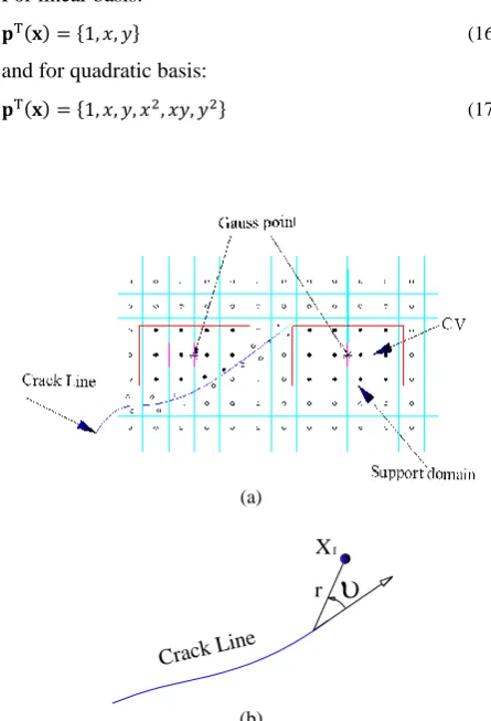
Figure 1. Definition the local domain in a tow-dimensional body
t
u
s
n
c
nC s
s
By substituting the Heaviside function as the weighting function in Equation (6), a domain integral in Equation (6) will be vanished, since . This results in reduction of computational cost in evaluating the integrals in Equation (6).
Also, as illustrated in Figure 1, the boundaries of CV may intersect with the global boundaries, i.e.
. Since both the free global
boundary and crack surface are free of traction, the corresponding integrals are vanished. Also, the first integral in Equation (6) can be cast to three parts: the one part of CV’s boundary which is inside the global domain, , the one part of CV’s boundary which intersects with the essential boundary, , and the one part of CV’s boundary which intersects with natural boundary, , thus we have:
∫ ∫ ∫ ∫ (8)
By substituting the constitutive equation as , in which is the elasticity matrix and is the strain vector defined in terms of the displacement as and also substituting Equation (3) in Equation (8) we have:
∫ ∫ ∫ ∫
(9)
The unknown displacement u can be approximated in terms of nodal parameters ̂ as:
̂ (10)
where is a matrix containing the interpolation functions related to the field nodes which are obtained by MLS method presented in the following Section. Substituting Equation (10) in to Equation (9) results in:
∫ ̂ ∫ ̂
∫
∫
(11)
Equation (11) represents the discretized form of equilibrium equation presented in Equation (1) for the CV corresponding to a field node. One can write this equation in the following well known form:
̂ (12a)
where and are the local stiffness matrix and local force vector, respectively, as follows:
∫ ∫
(12b)
∫ ∫
Equation (12) can be written for all the CVs constructed around the field nodes. The provided equations are assembled to form the global equation as follows:
(13)
where K, Fand U are the global stiffness matrix, global force vector and global displacement vector, respectively.
The essential boundary condition, Equation (3), in FVM can be enforced using the collocation technique [21]. Thus, the discretized Equation (12) for the CVs corresponding to the nodes located on the essential boundary can be replaced by the equations generated from the collocation technique for the constrained degrees of freedom as follows:
( ( )) ( ) (14)
2. 2. Moving Least Squares (MLS) Approximation In the MLS approximation, for a given set of nodal points scattered on the domain , the unknown function
( ) at a desired point in the domain is approximated continuously as follows [1]:
( ) ∑ ( ) ( ) ( ) ( ) (15)
where is the number of the basis functions. ( ) presents the vector of basis functions and can be selected as follows:
For linear basis:
( ) * + (16)
and for quadratic basis:
( ) * + (17)
(a)
(b)
Figure 2.(a) Definition the support domain for a gauss point on the face of a cell.(b) definition variables θ and r
X
rI
In Equation (15), ( ) is the associated unknown coefficient and , - is a vector of space coordinates. Coefficients in ( ) are obtained by minimizing a weighted discrete L2 norm as follows:
∑ ( ), ( ) ( )- ∑ (
),∑ ( ) ( ) ( )- (18)
( ) ( ) ( ) ̂ (19) where is the number of nodes in an area named as support domain which can be assumed as a rectangle shape centered at the desired point ,as shown in Figure 2. The dimensions of support domain, and , are determined as follows:
and (20)
which is the multiple factor of the average nodal spacing. The appropriate value for this coefficient is determined by numerical experiments [1].
In Equation (18), presents the weight function, which is equal to unity in the vicinity of point and zero on the edges of support domain. In this work, the quartic spline function is used as the weight function. This function is defined as follows:
( ) { ̅ ̅ ̅ ̅
̅ (21)
where ̅ , | | is the distance from node to the sampling point and is the size of support domain that is equal to and in x and y directions, respectively.
In Equation (19), ̂ is the vector of nodal parameter, and the moment matrix ( ) and matrix ( ) are defined by the following equations:
( ) ∑ ( ) ( ) ( ) (22)
( )
, ( ) ( ) ( ) ( ) ( ) ( )-
(23)
By solving Equation (19), ( ) is obtained as follows:
( ) ( ) ( ) ̂ (24)
Substituting Equation (24) in Equation (15) results in the following equation:
( ) ∑ ( ) ( ) ( ) ̂ (25)
where the interpolation function for ith node, , is defined as:
( ) ∑ ( )( ( ) ( ))
( )( ( ) ( )) (26)
It should be noted that if crack line passes across the support domain, according to visibility criterion [12], the nodes of support domain located in opposite of crack line take out from the support domain as shown in Figure 2.
3. COMPUTATIONAL MECHANICS OF CRACK GROWTH
3. 1. Calculation of Stress Intensity Factors Mainly three criteria are used to evaluate the crack growth: maximum circumferential stress criterion, maximum energy release rate criterion and minimum strain energy density criterion. In the present work, the maximum circumferential stress criterion is used [25]. According to this criterion, it is supposed that a crack in the direction perpendicular to the circumferential stress grows up. In other words, the crack growth occurs in the direction that the shear stress is zero. Hence, the angle of path of crack growth can be obtained by setting the shear stress of crack tip to zero which results in the following equation [9]:
( √
) (27)
in which and are the so-called stress intensity factors (SIF’s) corresponding to the first and second mode, respectively and is the angle of direction which crack growth occurs along with. Then, the equivalent SIF can be calculated using [9]:
(28) Computing SIFs for crack tips is a post-processing task in the analysis of crack growth problems. Therefore, after obtaining the displacement field of problem, one can calculate the SIF’s values for modes I and II of the crack tip.
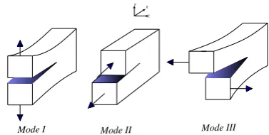
In Figure 3, the deformed shapes due to the different crack modes are displayed. Since in the present work the crack growth analysis is studied in the two dimensional bodies which are considered under the plane stress and plane strain states, the out-of-plane deformation of crack faces is omitted, therefore the first and second modes are considered.
Figure 3. Deformation in the different crack modes Y X
Z
The SIF factors can be obtained by using domain form of so-called interaction integral. This integral is derived from a path-independent integral known as J-integral using the following relations [26, 27]:
( ) ( ( ) ( )
( ) ( )) (29a)
where is defined as follows:
{ ( ) (29b)
and ( ) is interaction integral that is expressed as
follows [9]:
( ) ∫ ,
( ) ( )
( ) ( )
( )
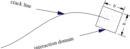
(30) in which variables superscripted by (1) are related to the actual state and variables superscripted by (2) are related to the auxiliary state. To calculate stress intensity factor corresponding to each mode, displacement and stress corresponding to the auxiliary fields of each mode should be substituted in Equation (30). One can gain auxiliary stress and displacement field from Westergard’s solution for stress and displacement fields of crack tip [28]. The domain of interaction integral is a square centered on the crack tip that its edges are set along with the last segment of crack increment (as shown in Figure 4).
3. 2. Quasi-Static Crack Growth Usually, two types of crack growth analysis are studied: quasi-static growth and fatigue crack growth. In the quasi-static type, after determining the direction of crack growth, a convenient increment value for the crack length must be considered. say about 0.1 , where is initial crack length [9]. A very small crack length increment assumption increases the time of analysis; On the other hand, assuming a large crack length increment leads to an inaccurate prediction of crack growth path. In this study, by using the numerical experiments, this value is considered about 0.1 , where is the last crack length. The fracture continues until the equivalent SIF obtained from Equation (28) exceeds the fracture toughness ( ) of material, which is obtained by experiments, i.e. . At this point, crack is unstable and analysis will be stopped.
Figure 4. Interaction integral domain
3. 3. Fatigue Crack Growth In the fatigue type of crack growth, to predict a crack increment value, the Paris law [29] is used which formulated as follows:
( ) ( ) in which C and m are material properties, is crack increment length, is number of loading cycles required to extend the crack from the last state to the new state with extended length. is called efficient
stress intensity factor and obtained by the following relation [29]:
( ) ( )
Using Equation (31) is possible in two ways, supposing the crack increment and calculating the number of load cycle or vice versa, supposing the number of load cycles and calculating the crack increment . Crack growth continues until , where is obtained from Equation (28) and is a material property named as the fracture toughness and is obtained by experiments as mentioned before. After reaching this limitation state, crack will be unstable and analysis is stopped.
3. 4. A Scheme for Dividing the CVs in the Crack Growth Analysis In the present approach for the crack propagation analysis, at the end of each step of analysis, the crack geometry is updated. Once the updated crack line enters a cell partially or passes it completely, the geometry of that cell is updated for the next step of analysis by splitting it to two separate cells. In case the crack line passes a cell completely, the division of that cell to two is obvious, but once the crack line just partially enters a cell, the last segment of the crack increment is extended virtually until it reaches the face of adjacent cell (see Figures 5a to 5c). By applying such scheme, the field node corresponding to the original cell is omitted and two new field nodes are considered at the center of the two newly generated cells. Also, it should be mentioned that for the cell partially passed by the crack line, by doing next step of analysis, the cell boundary aligned with the virtually extended part of the crack path is adjusted according to the new crack segment (see Figure 5(b)). It is understood that this cell dividing is easy to accomplish during the analysis and is not complicated. It should be noted that in the crack propagation analysis using the methods like finite element method, the traditional remeshing procedure is needed for producing a very fine mesh near the crack tip which is a burdensome task, hence researches have been encouraged to develop a new approach like XFEM. Also, in the XFEM method, a sub-triangulation scheme is needed near the crack tip in which a large number of Gauss points is used in each triangle [13]. Such triangulation task is avoided in the present method.
crack line b
b
(a)
(b)
(c)
Figure 5. Dividing the CVs during the crack growth.
4. NUMERICAL RESULTS
In the following section, some benchmark problems are solved using the present method and results are compared with the results obtained by other numerical and analytical methods.
4. 1. Edge Cracked Plate Under Tension In this problem an edged-cracked plate under pure tension, as a mode I crack propagation is analyzed using the present method (see Figure 6(a)). The length of plate is L=2, width W=1 and initial crack length a=0.2. The tensile stress on top and bottom sides of plate is . A finite volume model of plate consisting of 200 uniformly distributed cells is shown in Figure 6(b). A plane stress condition is assumed and also the elastic modulus and Poisson’s ratio are considered as E=207000 and , respectively. A quadratic basis functions has been used for the construction of shape functions using MLS technique. For evaluating the integrals on faces of cells, two Gauss points are used. Size of interaction-integral domain for various crack lengths is selected in the range of (0.3 to 0.85) . For evaluating the interaction
integral, the interaction domain is divided into a square mesh in which the quadrate Gauss points are used in every square. Table 1 shows the values of stress intensity factor for crack length varying from 0.2 to 0.5 where the error of the FVM predictions and also the predictions presented in Ref. [7] are calculated relative to the analytical results obtained by Tada et al. [30]. It can be seen that, using similar distribution of
nodes, the present FVM results have better accuracy comparing with the values obtained by the meshless method presented in Ref. [7]. Also, it should be noted that due to the fact that the problem is considered as a first mode cracking, the value of is obtained equal to
zero.
4. 2. Fatigue Crack Growth One of the important issues for the design of components of structures undergoing cyclic loading is the fatigue-life prediction. Hence, in the present test a problem of fatigue crack growth is studied by using the present method for an edge cracked plate under tension. Consider a rectangular plate with dimension including an inclined edge crack with angle of 40 degrees and length of 20 mm under cyclic loading on top and bottom sides as shown in Figure 7(a). This problem also has been solved by boundary element method in Ref. [31].
a b
Figure 6. Edge cracked plate under tension. (a) Geometry and loads; (b) Finite volume mesh
TABLE 1. Results for SIF in edge cracked problem with various crack length
a reference[7] FVM Analytical [30]
Error %- Reference[7]
Error%- FVM
0.2 1.07811 1.0884 1.08648 0.77 -0.18
0.24 1.25831 1.2734 1.27887 1.61 0.43
0.28 1.48169 1.4840 1.49354 0.79 0.64
0.32 1.72483 1.7255 1.73794 0.75 0.72
0.36 2.0611 1.9900 2.02186 -1.94 1.58
0.4 2.33212 2.3571 2.35802 1.10 0.04
0.44 2.78036 2.7870 2.76256 -0.64 -0.88
0.48 3.25899 3.2670 3.25542 -0.11 -0.36
0.49 3.40369 3.3949 3.39516 -0.25 0.01
0.5 3.52827 3.5401 3.54233 0.40 0.06
Crack geometry
crack tip- iteration i-1
crack tip- iteration i
Crack geometry
crack tip- iteration i+1
Crack geometry
nodes allocated to regular CVs nodes allocated to broken CVs
w
h h
a
The material properties are assumed the same as that used in that reference which are: the elasticity modulus, E=74000 MPa, the Poisson’s ratio, , the fracture toughness, . The plane stress
condition is assumed and the values of constants used in Paris law are, and m=3.32. The applied cyclic loading varying from a maximum value
of to a minimum value equal to zero. For
the construction of shape functions, the linear basis is used in MLS. Also, For evaluating the interaction integral, a square domain with sides equal to has
been used. Three different types of meshes i.e. ,
, and are used for the analysis of
fatigue crack growth. The problem domain is discretized initially to a uniform mesh of quadrilaterals according to the crack geometry. The mesh is used for defining the CVs where the two divided parts of each element cut by the crack line are used as two individual CVs, see Figure 7(b). By using the above three mesh densities, the fatigue crack growth is studied by assuming a constant crack increment equal to 5 units. The results are shown in Figure 8(a). It can be seen that how the crack growth path is affected by the mesh density.
(a) (b)
Figure 7. (a) Geometry and loading of an inclined edge cracked plate under cyclic loading; (b) discretized domain, using the mesh 1121
(a) (b)
Figure 8. (a) The crack growth path using different mesh densities; (b) Deformed shape at the final step of analysis using the mesh 2141
Figure 8(b) shows the displaced configuration of the plate corresponding to mesh , at the end of tenth as the final step of analysis. At the end of the last step, equivalent stress intensity, , reaches , so the
crack is unstable and analysis is stopped. To investigate the effect of crack increment value assumed in each step of analysis on the path of crack growth, the problem is analyzed using different crack increment values corresponding to mesh . The predicted geometry of crack growth is shown in Figure 9. It can be seen that assuming the crack increments lesser than the dimension of CV leads to inaccurate path for crack growth.
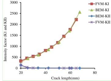
In Figures 10 and 11, fatigue-life diagram and
values in terms of crack growth are compared
with the results presented in Ref. [31] that have been obtained using boundary element method (BEM). It can be observed that the results obtained by the present method are in good agreement with the reference results. Also, it can be seen that the present method is able to predict the fracture due to fatigue crack growth with a reasonable accuracy.
4. 3. Crack Growth under Mixed Mode Investigation of crack growth trajectory is one of the important problems in the fracture analysis of structures.
Figure 9. predicted path for growth of edge inclined crack using various crack increment
Figure 10. Variations of SIF’s in term of crack extension
20 m m
40 N/mm2
200 mm
100 mm -1000 10 20 30 40 50 60 70 80 90 100
-80 -60 -40 -20 0 20 40 60 80 100
Nodal distribution (11X21)=235
0 2 4 6 8 10 12 14 16 18
0 20 40 60
y
(m
m
)
x(mm)
FVM-11*21 Nodes
FVM-15*29 Nodes
FVM-21*41 Nodes
0 2 4 6 8 10 12 14 16
0 10 20 30 40 50 60
Intensit
y
fa
ctor
(K
1
and KI
I)
Crack length(mm)
crack increment=2 units crack increment=5 units crack increment=7.5 units crack increment=10 units
0 500 1000 1500 2000 2500 3000
20 40 60 80
Intensit
y
fa
ctor
(K
1
and KI
I)
Crack length(mm)
FVM-KI
BEM-KI
BEM-KII
Figure 11. Fatigue-life diagram for inclined edge cracked plate under cyclic loading
In this test, the path of a crack growth in the mixed mode conditions is presented. Consider an edge cracked plate under shear stress, , applied on top and fixed at the bottom as shown in Figure 12. Dimensions of plate are: length L=8 in., width W=7 in. and crack length a=3.5 in. The plate domain is discretized to 253 cells using a mesh of 1129 with uniformly spaced centers except ones passed by crack line that are divided into two cells in both sides of crack line. The crack increment in each step is assumed 0.3 in. The plane stress condition is assumed and quadratic basis function is used for the construction of shape functions. Also, for evaluating the integrals relating to the internal forces on CVs’ faces, two Gauss points are considered on cell faces. Domain size used for the calculation of interaction integral is varied between
and . This variation in the domain size is needed
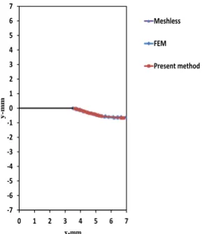
to avoid interference of plate boundaries in the computation of interaction integral when crack tip approaches plate edges; otherwise, interaction integral are calculated inaccurately which results in wrong crack path. The trajectory of crack growth and also the final deformed shape of plate after 23 steps are displayed in Figures 13. The path of crack growth obtained by the meshless method and finite element method [32] are also presented in Figure 13. As can be seen, the crack growth path obtained by FVM has good agreement with the predictions by the two other methods. This result indicates the capability of the present method in estimation of crack growth path in problems involving both modes I and II of cracks.
5. CONCLUSION
In this work the finite volume method has been extended for crack growth analysis in two dimensional bodies.
In this extended form of FVM, the MLS technique is used for the construction of interpolation functions for the integration points considered on cell boundaries. Several problems have been solved by this method and the results have been compared with the analytical, numerical and experimental results. The comparisons have shown that the predictions of the present method have good agreement with the reference results for SIF calculations and crack growth path predictions. One of the interesting features of the presented finite volume method is that in each step of analysis, due to crack growth, only cell dividing near the crack tip is needed which can be implemented easily rather than extensive remeshing which is needed in the finite element method. Also, the present study reveals the great potential of FVM for the fracture analysis of structures with a prospect of application for the existed challenges in the dynamic crack propagation.
Figure 12. (a) Ggeometry and loading of an edge cracked plate under Mixed mode; (b) displaced geometry of plate in the final step of analysis
Figure 13. Crack growth trajectory in a plate under mixed mode loading
0 10 20 30 40 50 60 70 80
0 50,000 100,000 150,000 200,000
C
ra
ck
leng
th(mm
)
Number of cycle loading
BEM
FVM
7in
8in 8in
3.5in
-7 -6 -5 -4 -3 -2 -1 0 1 2 3 4 5 6 7
0 1 2 3 4 5 6 7
y
-mm
x-mm
6. REFERENCES
1. Belytschko, T., Lu, Y.Y. and Gu, L., "Element‐free galerkin methods", International Journal for Numerical Methods in
Engineering, Vol. 37, No. 2, (1994), 229-256.
2. Liu, W.K., Jun, S. and Zhang, Y.F., "Reproducing kernel particle methods", International Journal for Numerical
Methods in Fluids, Vol. 20, No. 8‐9, (1995), 1081-1106.
3. Armando, D. and Oden, J., "Hp clouds-a meshless method to solve boundary value problems." (1995): TICAM Report, University of Texas at Austin. 95-105.
4. Melenk, J.M. and Babuška, I., "The partition of unity finite element method: Basic theory and applications", Computer
Methods in Applied Mechanics and Engineering, Vol. 139,
No. 1, (1996), 289-314.
5. Atluri, S.N. and Zhu, T., "A new meshless local petrov-galerkin (mlpg) approach in computational mechanics", Computational
Mechanics, Vol. 22, No. 2, (1998), 117-127.
6. Oñate, E., Perazzo, F. and Miquel, J., "A finite point method for elasticity problems", Computers & Structures, Vol. 79, No. 22, (2001), 2151-2163.
7. Belytschko, T., Gu, L. and Lu, Y., "Fracture and crack growth by element free galerkin methods", Modelling and Simulation
in Materials Science and Engineering, Vol. 2, No. 3A, (1994),
519.
8. Belytschko, T. and Tabbara, M., "Dynamic fracture by the element-free galerkin method", ASME-PUBLICATIONS-PVP, Vol. 294, No., (1994), 159-159.
9. Fleming, M., "The element-free galerkin method for fatigue and quasi-static fracture", Doctor of Philosophy Thesis,
Northwestern University, (1997).
10. Xu, Y. and Saigal, S., "An element free galerkin formulation for stable crack growth in an elastic solid", Computer Methods in
Applied Mechanics and Engineering, Vol. 154, No. 3, (1998),
331-343.
11. Krysl, P. and Belytschko, T., "The element free galerkin method for dynamic propagation of arbitrary 3‐d cracks", International
Journal for Numerical Methods in Engineering, Vol. 44, No.
6, (1999), 767-800.
12. Fleming, M., Chu, Y., Moran, B., Belytschko, T., Lu, Y. and Gu, L., "Enriched element-free galerkin methods for crack tip fields", International Journal for Numerical Methods in
Engineering, Vol. 40, No. 8, (1997), 1483-1504.
13. Dolbow, J. and Belytschko, T., "A finite element method for crack growth without remeshing", International Journal for Numerical Methods in Engineering, Vol. 46, No. 1, (1999), 131-150.
14. Shen, S.N.A. and Shengping, "The meshless local petrov-galerkin (mlpg) method: A simple & less-costly alternative to the finite element and boundary element methods", Computer Modeling in Engineering & Sciences, Vol. 3, (2002), 11-51. 15. Onate, E., Cervera, M. and Zienkiewicz, O., "A finite volume
format for structural mechanics", International Journal for Numerical Methods in Engineering, Vol. 37, No. 2, (1994), 181-201.
16. Ivankovic, A., Demirdzic, I., Williams, J. and Leevers, P., "Application of the finite volume method to the analysis of
dynamic fracture problems", International Journal of
Fracture, Vol. 66, No. 4, (1994), 357-371.
17. Ivankovic, A., Muzaferija, S. and Demirdzic, I., "Finite volume method and multigrid acceleration in modelling of rapid crack propagation in full-scale pipe test", Computational Mechanics, Vol. 20, No. 1-2, (1997), 46-52.
18. Fallah, N., Bailey, C., Cross, M. and Taylor, G., "Comparison of finite element and finite volume methods application in geometrically nonlinear stress analysis", Applied Mathematical
Modelling, Vol. 24, No. 7, (2000), 439-455.
19. Stylianou, V. and Ivankovic, A., "Finite volume analysis of dynamic fracture phenomena–i. A node release methodology",
International Journal of Fracture, Vol. 113, No. 2, (2002), 107-123.
20. Stylianou, V. and Ivankovic, A., "Finite volume analysis of dynamic fracture phenomena–ii. A cohesive zone type methodology", International Journal of Fracture, Vol. 113, No. 2, (2002), 125-151.
21. Atluri, S., Han, Z. and Rajendran, A., "A new implementation of the meshless finite volume method, through the mlpg “mixed” approach", CMES: Computer Modeling in Engineering &
Sciences, Vol. 6, No. 6, (2004), 491-514.
22. Moosavi, M., Delfanian, F. and Khelil, A., "Orthogonal meshless finite volume method applied to crack problems",
Thin-Walled Structures, Vol. 52, (2012), 61-65.
23. Ebrahimnejad, M., Fallah, N. and Khoei, A., "New approximation functions in the meshless finite volume method for 2d elasticity problems", Engineering Analysis with
Boundary Elements, Vol. 46, (2014), 10-22.
24. Mahmoodabadi, M., Sarfarazi, M., Bagheri, A. and Baradaran, G., "Meshless local petrov-galerkin method for elasto-static analysis of thick-walled isotropic laminated cylinders",
International Journal of Engineering-Transactions B:
Applications, Vol. 27, No. 11, (2014), 1731.
25. Erdogan, F. and Sih, G., "On the crack extension in plates under plane loading and transverse shear", Journal of Basic
Engineering, Vol. 85, No. 4, (1963), 519-525.
26. Rice, J.R., "A path independent integral and the approximate analysis of strain concentration by notches and cracks", Journal
of Applied Mechanics, Vol. 35, No. 2, (1968), 379-386.
27. Moran, B. and Shih, C., "Crack tip and associated domain integrals from momentum and energy balance", Engineering
Fracture Mechanics, Vol. 27, No. 6, (1987), 615-642.
28. Westergaard, H., "Bearing pressures and cracks", Journal of
Applied Mechanics, Vol. 6, (1939), 49–53.
29. Paris, P. and Erdogan, F., "A critical analysis of crack propagation laws", Journal of Basic Engineering, Vol. 85, No. 4, (1963), 528-533.
30. Tada, H., Paris, P.C. and Irwin, G.R., "The stress analysis of cracks", Del Research Corp, Hellertown PA, (1973).
31. Yan, A. and Nguyen-Dang, H., "Multiple-cracked fatigue crack growth by bem", Computational Mechanics, Vol. 16, No. 5, (1995), 273-280.
A Development in the Finite Volume Method for the Crack Growth Analysis without
Global Remeshing
A. Amraei, N. Fallah
Department of Civil Engineering, University of Guilan, Rasht, Iran
P A P E R I N F O
Paper history: Received 24 March 2016
Received in revised form 25 May 2016 Accepted 02 June 2016
Keywords: Crack Growth Interaction Integral Finite Volume Moving Least Squares
ديكچ ه
ٌساس تسکض کیواکم رد راًضد لئاسم سا یکی ترًص ٍب کزت ذضر لیلحت یفزط سا .تسا ٌذوام یقاب اَ
، کزت ذضر
ٌساس رد لياذتم یا ٌذیذپ ،یگتسخ یتطک ،اَامیپاًَ لاب نًچمَ ییاَ
یم تاعیام نساخم ي اَ تسکض زثا یسرزب اذل .ذضاب
و هیا سا یضاو ٌساس ٍوًگ هیا یحازط رد یگدرًخ کزت عً
یريزض اَ تس ديذحم مجح شير قیقحت هیا رد . یازب
لذم
یم ٌداد ٍعسًت یذعب يد لئاسم رد یگتسخ ي یکیتاتسا کزت صخپ ندًمو دذجم یذىب صم ٍب یسایو زضاح شير رد .دًض
کزت ذضر سا ٍلحزم زَ رد ٍلاسم لک ،تسیو
لًلس طقف ي ت کزت کًو رد عقاي یاَ
یم میسق ب زما هیا ي ذودزگ ٍ
رد یگداس
یم ترًص شیلاوآ یط یم ٍعلاطم ٍلاسم هیذىچ لح اب یداُىطیپ شير تقد .دزیگ
ي یلیلحت جیاتو اب لصاح جیاتو .ددزگ
ٍسیاقم دًجًم یدذع جیاتو ي ٌذض
یم ٌذَاطم ٍک دًض هیا .ذضاب یم عجزم جیاتو اب ٍسیاقم رد یبًخ تقد یاراد جیاتو